Contents lists available atSciVerse ScienceDirect
Computers and Mathematics with Applications
journal homepage:www.elsevier.com/locate/camwa
Multilayer perceptrons and radial basis function neural network
methods for the solution of differential equations: A survey
Manoj Kumar, Neha Yadav
∗Department of Mathematics, Motilal Nehru National Institute of Technology, Allahabad-211004 (U.P.), India
a r t i c l e i n f o Article history:
Received 29 April 2011
Received in revised form 8 August 2011 Accepted 14 September 2011 Keywords:
Differential equations Neural network Multilayer perceptron Radial basis functions Backpropagation algorithm
a b s t r a c t
Since neural networks have universal approximation capabilities, therefore it is possible to postulate them as solutions for given differential equations that define unsupervised errors. In this paper, we present a wide survey and classification of different Multilayer Perceptron (MLP) and Radial Basis Function (RBF) neural network techniques, which are used for solving differential equations of various kinds. Our main purpose is to provide a synthesis of the published research works in this area and stimulate further research interest and effort in the identified topics. Here, we describe the crux of various research articles published by numerous researchers, mostly within the last 10 years to get a better knowledge about the present scenario.
©2011 Elsevier Ltd. All rights reserved.
1. Introduction
A series of problems in many scientific fields can be modeled with the use of differential equations such as problems in physics [1–3], chemistry [4–6], biology [7,8], economics [9], etc. Due to the importance of differential equations many methods have been proposed in the relevant literature for their solution such as Runge–Kutta methods [10,11], Predictor–Corrector methods [12,13], Finite Difference methods [14–16], Finite Element methods [17–19], Splines [20–23] and other methods [24–41] etc. These methods require the discretization of domain into the number of finite elements where the functions are approximated locally. Although these methods provide good approximations to the solution, they require a discretization of domain via meshing, which may be challenging in two or higher dimension problems. Also, the approximate solution derivatives are discontinuous and can seriously impact on the stability of the solution. Furthermore, in order to obtain satisfactory solution accuracy, it may be necessary to deal with finite meshes that significantly increase the computational cost.
In spite of the above methods, approximate particular solutions can also be achieved by using multilayer perceptrons, radial basis functions, models based on genetic programming, hybrid approaches based on neural networks, etc. Advantages of these methods are that they involve a single independent variable regardless of the dimension of the problem, and the solution obtained from the neural network methods are differentiable and in closed analytic form. During the last few years much progress has been done in this area. In this article, a wide survey of solution of differential equations using multilayer perceptrons (MLP) and radial basis functions (RBF) along with our own comparative remarks have been presented. We will omit the details of techniques used to solve these models due to length constraints. Interested readers can see the references cited (along with these methods) for more details.
The rest of this article is organized as follows: in Section2, we present a summary of Multilayer perceptron (MLP) neural network techniques for solving differential equations from various research articles. A brief description of articles published on the Radial Basis function neural network (RBFN) technique for solving differential equations is presented in Section3. In
∗Corresponding author.
E-mail addresses:[email protected](M. Kumar),[email protected](N. Yadav). 0898-1221/$ – see front matter©2011 Elsevier Ltd. All rights reserved.
Section4, a comparison of MLP and RBF techniques for solving differential equations are given. Finally, Section5presents major conclusions and further developments.
2. Multilayer perceptron (MLP) neural network techniques to solve differential equations
In this section, we will give a brief description of multilayer perceptron (MLP) neural network techniques for solving differential equations of various kinds. Various research articles considered here are in the ascending order of their years of publication.
In [42], Meadre and Fernandez concentrated on developing a general, numerically efficient, non-iterative method in which the feed forward artificial neural network architecture can be used to model the solution of algebraic and differential equations accurately, using only the equation of interest and the boundary or initial conditions. A feed forward artificial neural network (FFANN) constructed by this non-iterative method is indistinguishable from those methods which are trained using conventional techniques. They borrowed a technique from applied mathematics, known as the method of weighted residuals (MWR), and showed how it can be made to operate directly on the network architecture. The method of weighted residuals is a generalized method for approximating functions, usually from given differential equations. A simple feed forward network using a single input and output neuron with a single hidden layer of processing elements utilizing the hard limit transfer function is constructed to approximate accurately the solution of a first and second order linear ordinary differential equation. They also predicted and controlled the error constructed by feed forward artificial neural networks. The non-iterative approach outlined in the article has allowed suitable algorithms to be devised for the synthesis of FFANNs that approximate non-linear ordinary differential equations. Also the non-iterative algorithm has allowed work to progress in the construction of FFANNs, sigma-Pi, and recurrent networks, to approximate linear and non-linear partial differential equations.
Remark 1. It can be concluded from the above article that it is possible to construct directly and non-iteratively a feed forward neural network to approximate arbitrary linear ordinary differential equations. The methods used are all linear in storage and processing time. TheL2—norm of the network approximation error decreases quadratically with the increasing number of hidden neurons. The result obtained through the output of network demonstrates the accuracy of approximation. In the research article [43], Issac Ellias Lagaris and Aristidis Likas presented a new method for solving initial and boundary value problems using artificial neural network. To illustrate their method they took the following general differential equation:
G
(
⃗
x, ψ(
⃗
x),
∇
ψ(
⃗
x),
∇
2ψ(
⃗
x))
=
0,
⃗
x∈
D (1)subject to the certain boundary conditions which are either Dirichlet or Neumann boundary conditions. Also
⃗
x=
(
x1,
x2, . . . ,
xn)
∈
Rndenotes the definition domain andψ(
⃗
x)
is the solution to be computed. Collocation method is adopted,to obtain a solution of the above differential equation(1), which assumes the discretization of the domainDandSintoD
ˆ
andˆ
S. Solve the above differential equation. They choose the form of trial function
ψ
t(
⃗
x)
such that by construction it satisfiesthe given boundary conditions. This is obtained by writing the trial function as a sum of two parts
ψ
t(
⃗
x)
=
A(
⃗
x)
+
F(
⃗
x,
N(
⃗
x,
⃗
p))
(2)whereN
(
⃗
x,
p⃗
)
is a single output feed forward neural network with parameters⃗
pandninput units fed with the input vector⃗
x. TermA
(
⃗
x)
contains no adjustable parameters and satisfies the boundary conditions. The second termFemploys a neural network whose weights are adjusted to deal with the minimization problem and it is constructed so as not to contribute with boundary conditions. Then the network is trained to satisfy the differential equation. The authors illustrated present method by solving a variety of model problems. The solution such obtained is compared with the solution obtained using the Galerkin finite element method for several cases of partial differential equations and it is found that the method exhibits excellent generalization performance since the deviation at the test points was ‘in no case’ greater than the maximum deviation at the training points.Remark 2. Method presented by the authors in [43] is general and can be applied to ordinary differential equations, the system of coupled ordinary differential equations and also to partial differential equations. It is also stressed out that the present method described in [43] can easily be used for dealing with the domains of higher dimensions. The method becomes particularly interesting with the help of neuroprocessor due to expected essential gains in the execution speed.
In article [44], the authors presented a method to solve a class of first order partial differential equation as input to state linearizable or approximate linearizable system. They proposed an extended backpropagation algorithm for training the derivative of a feed forward neural network and further, an approximate solution for a class of partial differential equation is obtained. A feedback control law has been designed to control a class of non-linear systems, based on the approximate solution. Simulation technique is used to demonstrate the effectiveness of the proposed algorithm and it is shown that the method can be very useful for practical applications in the following cases:
I. When a non-linear system satisfies the conditions for input-to-state linearization but the non-trivial solution of the given equation
∂λ(
x)
∂
x
g(
x)
ad1fg(
x) . . .
adfn−2g(
x)
=
0 (3)is hard to find by training the derivative of a neural network. We can seek the approximate solution by the method given in [44]. Since there is no restrictive condition for choosing the basis vector to train the neural network, therefore a simple transformation to construct the basis is recommended.
II. When a non-trivial solution does not exist for the above given equation, we still obtain an approximate solution. If the approximate solution is considered an exact solution for a linearizable feedback system, then the system should approximate the given non-linear system as closely as possible.
Remark 3. It is pointed out that the method presented in [44] can benefit the design of the class of non-linear control systems, when the non-trivial solution of partial differential equations is difficult to find. Simulation examples presented in the article exhibit the advantages and effectiveness of the method. For applications where a large region of operation is required, the control design based on this method cannot result in a satisfactory performance.
Lagaris et al. in [45] studied partial differential equation with the case of complex boundary geometry. They examined the partial differential equations of the form
LΨ
=
f (4)whereLis a differential operator andΨ
=
Ψ(
⃗
x)(
⃗
x∈
D⊂
R(n))
with Dirichlet or Neumann boundary conditions. TheboundaryB
=
∂
Dcan be any arbitrary complex geometrical in shape and is defined as a set of points that are chosen so as to represent its shape with reasonable accuracy. Collocation method is adopted and the problem is then transformed into the unconstrained optimization problem. A model based on the synergy of two feed forward neural networks of two different types are developed, which can be written asΨM
(
⃗
x,
p)
=
N(
⃗
x,
p)
+
M−
l=1 qle−λ|⃗x−α ⃗ rl+⃗h|2 (5)where
|·|
denotes the Euclidean norm andN(
⃗
x,
p)
is a multilayer perceptron withpdenoting the set of its weights and biases. The sum in the above equation represents an RBF network with M hidden units that all share a common exponential factorλ
. For a given setpof MLP parameters, the coefficientsqlare uniquely determined by requiring that the boundary conditions aresatisfied. The authors demonstrated that the model based on the MLP-RBF synergy satisfies exactly the boundary conditions but are computationally expensive since at every evaluation of the model one needs to solve a linear system which may be quite large. Moreover, since many efficient optimization methods need the gradient of the objective function, one has to solve an additional linear system of the same order for each gradient component. On the other hand, penalty method is very efficient but does not satisfy the boundary conditions. Hence they used the combination of these two methods which is profitable and results are quite encouraging. They presented three examples to illustrate their method, the first example is a two dimensional linear Dirichlet problem on a irregular body. The second example is a highly non-linear problem with Dirichlet boundary problem considering star shaped domain, and the third example treats the same PDE with Neumann boundary conditions inside a cardioid family.
Remark 4. Solutions obtained by the given approach show that the method is equally effective, and retains its advantage over the Galerkin Finite element method. It also provides accurate solutions in a closed analytic form that satisfy the boundary conditions at the selected points. The method is quite general and can be used for a wide class of linear and non-linear partial differential equations.
In article [46], the authors described a method to solve partial differential equation and its boundary or initial conditions by using neural networks. They used the fact that multiple input, single output and single hidden layer feed forward networks with a linear output layer with no bias are capable of arbitrarily well approximating arbitrary functions and its derivatives. To clarify the working of their method, they apply the following differential equation with two of its initial conditions:
d2y
dt2
+
y=
0,
t∈ [
0,
1]
(6)dy
dt
=
1,
y(
0)
=
0.
(7)Then, they obtain networks of which some are specifically structured. To find the solution of the partial differential equation and its boundary and initial conditions they trained all obtained networks simultaneously as a consequence of their interrelationship. For this they implemented evolutionary algorithm to train the networks. They noticed that good results can be obtained if they restrict the values of the variables to the interval [
−
5, 5].Remark 5. The authors presented the knowledge about the partial differential equations and its boundary and/or initial conditions to incorporate into the structures and the training sets of several neural networks and found that the results for one and two dimensional problem are very good in respect of efficiency, accuracy, convergence and stability.
Alli et al. in [47] solved a mathematical model of vibration control of flexible mechanical systems, using multilayer perceptron technique. Because of non-linearity and complex boundary conditions, their numerical solutions always have some drawbacks such as numerical instability. That is why, they proposed an alternative method using feed forward artificial neural networks. Initially a general formula for the numerical solutions ofnth order initial value problem is developed using ANN. Then the method is applied to many controlled and non-controlled vibration problems of flexible structures whose dynamics are represented by ODE’s and PDE’s, for e.g., they considered mass-damper-spring system, whose mathematical model is given by:
md 2
ψ
dt2+
cd
ψ
dt
+
kψ
=
0 (8)where the initial conditions of the systems are:
ψ(
0)
=
1 and dψ(dt0)=
0 witht∈ [
0,
2]
. The authors also considered the second and fourth order PDEs that are the mathematical models of the control of longitudinal vibrations of rods and lateral vibration of beams. To test their method, they also obtain the solutions of the same problems by using analytical and Runge–Kutta method. The obtained figures show that the results are very closed to the Runge–Kutta and analytical method. Remark 6. It has been pointed out that the method presented in [47] can be used for a wide class of linear and non-linear PDEs with complex boundary conditions and the results obtained are very good. It has been also observed that the presented method also success outside the training points when the neuron numbers in the hidden layer are increased.Smaoui et al. in [48] analyzed the dynamics of two non-linear partial differential equations known as the Kuramato–Sivashinsky (K–S) equation and the two dimensional Naiver–Stokes (N–S) equation using the combination of Karhunen–Loeve (K–L) decomposition and artificial neural networks. K–S equation is solved using pseudo spectral Galerkin method at bifurcation parameters
α
=
17.
75. K–L decomposition was thus applied on the numerical simulation data to extract coherent structures of the dynamical behavior represented by heteroclinic connection. The author then used the artificial neural network to model and predictPtimes steps into the future dynamical behavior atα
=
17.
75 for different values ofP. They found that the neural network model is able to capture the dynamics, and observed that asPincreases, the model behavior degrades. And for the two dimensional N–S equation, a quasiperiodic behavior represented in phase space by a torus is analyzed at Re=
14:
0. Applying the symmetry observed in the two-dimensional N–S equations on the quasiperiodic behavior, eight different tori were obtained. They showed that by exploiting the symmetries of the equation and using K–L decomposition in conjunction with neural networks, a smart neural model can be obtained.Remark 7. In [48], the authors presented a hybrid method which is the combination of K–L decomposition and artificial neural network, to solve the partial differential equations. They established a foundation for modeling the two dimensional N–S equation using neural network for all values of Reynolds numbers and for different values of wave numbers.
In [49] Malek et al. investigated a novel hybrid method based on optimization techniques and neural network methods for the solution of high order ordinary differential equations. The authors considered the general initial/boundary value problem of the form:
D[
x,
y(
x),
dy dx,
d2y dx2, . . . ,
dny dxn]
=
0 x∈ [
a,
b]
C[
x,
y(
x),
dy dx,
d2y dx2, . . . ,
dny dxn]
=
0 x=
aand/
orb (9)whereDis a differential operator of degreen
,
C is an initial/boundary operator,xis an independent variable belonging to[
a,
b]
andyis an unknown dependent variable to be calculated. For problem formulation, they assume that a general approximation solution to Eq.(9)is of the formyT(
x,
P)
whereyTis a dependent variable toxandP, wherePis an adjustableparameter involving weights and biases in the structure of three layer feed forward neural networks and satisfies the following optimization problem:
Min P∫
b a
D[
x,
yT(
x,
P),
dyT(
x,
P)
dx, . . . ,
dnyT(
x,
P)
dxn]
2 dx C[
x,
yT,
dyT(
x,
P)
dx, . . . ,
dny T(
x,
P)
dxn]
=
0,
x=
aand/
orb.
(10)In order to deal with Eq.(10)it is simpler to deal the following constrained optimization problem of the formyT
(
x,
P)
=
α(
x)
+
β
[
x,
N(
x,
P)
]
, where first term involve adjustable parameters and satisfy initial or boundary conditions and second term is feed forward three layer perceptron. Minimization in Eq.(10)has been done which is considered as a training process for the proposed neural network. The errorE(
x)
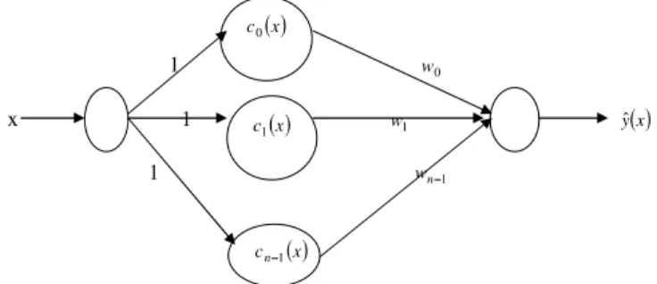
corresponding to every entryxhas to be minimized. The authors described,Fig. 1. Neural Network based on cosine based model.
the general formulation of initial or boundary value problems by taking differential equations of various order. They developed programs with MATLAB 6.5.1 to demonstrate behavior and properties of the proposed method and concluded that the proposed novel solution act as a good interpolation technique as well as a good extrapolation method for the close enough point outside the boundary points of the interval.
Remark 8. The main contribution of this article [49] is the potential of the hybrid technique to deal with differential equation of higher orders as well as low order. This hybrid technique is applicable for partial differential equation as well as ordinary differential equation and numerical simulation indicates that the proposed novel model solution is stable and computes the approximate solution in few numbers of iterations. Moreover, it acts as a good extrapolation technique for a good range of points outside the interval
[−
1,
1]
.An algorithm for the selection of both input variables and a sparse connectivity of the lower layer of connections in feed forward neural network of multilayer perceptron with one layer of hidden non-linear single linear output node is presented by Saxen et al. in [50]. Initially random weights in the lower layer of connections are used as a starting point and the complexity of this part of the network is gradually decreased. At every step of the algorithm, least significant connection is eliminated by a procedure, where the lower layer weights are zeroed, in turn, and the network corresponding to minimum approximation error is selected. In carrying out the comparison between the networks, the upper layer connection weights are determined by linear least squares, this feature made the method efficient and robust. The results of the algorithm are saved in a book-keeping matrix that can be interpreted in retrospect to suggest a suitable set of inputs and connectivity of the lower part of the network. Various test examples are presented by the authors to illustrate that the proposed algorithm is a valuable tool for the users in extracting relevant inputs from a set of potential ones.
Remark 9. This method is a systematic method that can guide the selection of both input variables and sparse connectivity of the lower layer of connections in feed forward neural networks of multi-layer perceptron type with one layer of hidden non-linear units and a single linear output node and the algorithm developed for the method is efficient, rapid and robust.
In article [51], the authors emphasized on solving the first order initial value problem in ordinary differential equations. They used the cosine function as the transfer function of neural network and supposed the error function is e
(
x)
=
f
(
x,
yˆ
(
x))
− ˆ
y′(
x)
; and madee(
x)
→
0 by training neural network. Thus, theyˆ
(
x)
approximate toy(
x)
. The model of neuralnetwork based on the cosine basis function is shown inFig. 1. Here,
w
nis weight vector,cn(
x)
=
∑
N−1n=0cos
(
nx)
is transfer function of the hidden layer neuron,x∈ [
0, π
]
, weight matrix vector isW= [
w
0, w
1, . . . , w
n−1]
T and transfer function matrix asc(
x)
=
(
c0(
x),
c1(
x), . . . ,
cn−1(
x))
T,
Nis the number of hidden layer neurons and Neural network output is given as ;ˆ
y(
x)
=
N−1−
n=0ω
ncosnx.
(11)They developed a neural network algorithm, by considering the initial value problems in ordinary differential equations, for which weight is adjusted as;
w
n(
k+
1)
=
w
n(
k)
= −
µ
e(
k)
[
nsinnxk+
fy(
x,
yˆ
(
xk)
cosnxk)
]
n=
0,
1, . . . ,
N−
1 (12)where
µ
is learning rate and 0< µ <
1.They also described convergence criteria for neural network algorithm in terms of the following theorem:Theorem. Suppose that
µ
is the learning rate, N is the number of hidden layer neurons, L is the upper limit of ∂f(∂xy,y). Then
∂f(x,y) ∂y
≤
L. If learning rate satisfies0< µ <
12
N(2N2+6L2−3N+1), then the algorithm is convergent.
Then, the author tested the validity of the algorithm on a plenty of examples and compare the results with the other existing methods. They found that the algorithm is more precise, it provides a new approach on numerical computation, also it can give results at an arbitrary x between two adjacent nodes.
Remark 10. As per the results given in the article [51], it has been observed that the proposed algorithm is more precise than the Euler Method, Modified Euler Method and Heun’s Method. However, compared to Runge–Kutta method of order four, the results of calculation are less precise but method is more flexible than any other difference methods.
In [52] the authors presented the numerical solution of non-linear Schrodinger equation by feed forward neural network. They considered the following time independent Schrodinger equation of the motion of a quantum particle in a one dimensional system:
ˆ
Hψ(
x)
≡
−
h 2 2m∂
2∂
x2+
V(
x)
ψ(
x)
=
Eψ(
x)
(13)wheremandV
(
x)
are the mass of a particle and the potential function, respectively.Hˆ
, ψ(
x)
, andEdenote the system Hamiltonian, Eigen function and the Eigen value, respectively. The identity of quantum mechanical state can be represented by the wave functionψ(
x)
=
A(
x)
.S(
x)
in the coordinate system. The authors represented the wave function by the feed forward artificial neural network, in which the coordinate value is regarded as an input while the networks output are assigned to two separate parts. They obtained energy function of the artificial neural network from the Schrodinger equation and its boundary conditions and used unsupervised training method for training the network. The present method is applied to the quantum infinite square well and one dimensional quantum harmonic oscillator systems and the result proves its wide applicability. The authors compared the accuracy of their method by comparing the results to the results that are analytically known and also by the Runge Kutta method of order four.Remark 11. It has been pointed out that the method presented in [52] can solve the Schrodinger equation effectively with small number of unknown parameters in comparison with the other conventional methods e.g. Runge Kutta, Finite difference etc. The method can be used for dealing with the higher dimensions also.
In [53], the author proposed a hybrid method based on artificial neural networks, minimization techniques and collocation method to determine a related approximate solution in a closed analytic form of the time independent partial differential equations containing several arbitrary and boundary conditions of the form:
∀
i1=
1, . . . ,
p1:
Di1[
t,
x, . . . ,
∂
α0+α1+···+αn∂
tα0∂
xα1 1· · ·
∂
xα n n yi(
t,
x), . . .
]
=
0,
t∈ [
t0,
tmax]
,
x∈
Ω∀
i2=
1, . . . ,
p2:
Ii2[
t0,
x, . . . ,
∂
α0+α1+···+αn∂
tα0∂
xα1 1. . . ∂
x αn n yi(
t0,
x), . . .
]
=
0,
x∈
Ω,
1≤
i≤
m∀
i3=
1, . . . ,
p3:
Bi3[
t,
x, . . . ,
∂
α0+α1+···+αn∂
tα0∂
xα1 1. . . ∂
xα n n yi(
t,
x), . . .
]
=
0,
t∈ [
t0,
tmax]
,
x∈
Ω (14)where the real valued multivariable functionsDi1
,
Ii2andBi3represents the known and non-linear time dependent system of partial differential equations, initial and boundary conditions, respectively,tis the time variable, x is the real valued spatial variable,Ω⊆
Rnis a bounded domain,(α
0, α
1, . . . , α
n)
∈
Nn+1
0
(
N0=
N∪ {
0}
)
is multi index variable. They establish a trial approximate solutionyT(
t,
x,
P)
= [
yT1(
t,
x,
P1), . . . ,
yTm(
t,
x,
Pm)
]
according to Kolmogorov and Cybenko theorems [54,55] that includesmthree layered feed forward neural networks and contains adjustable parameters for the solution. The authors also proposed a specific trial solution for the bi-harmonic problem in order to simplify the corresponding energy function that must be minimized; they obtained mixed partial derivatives for the output of neural networks using multi index representation. The method is illustrated on various examples that involve a direct technique of the Nelder–Meed method [56] for optimization and the approximate solution obtained is in closed analytic form which works well for the points inside and outside the problem domain near boundary points.Remark 12. The method proposed by the authors in the article [53] provides the approximate solution in a closed analytic form. Some advantages of this approach are that, it can solve the time dependent systems of partial differential equations, the method is generalized for solving the higher order and non-linear problems, it deals with a few number of parameters, solution is fast evaluated, the method can be applied to initial and two point boundary value problem for ordinary differential equations, and it uses parallel processing. Unlike the other methods, there is no ill conditioning of the concluded linear system in the expansion methods or the necessity of making a special relation among the step size for different axis in the finite difference method.
In [57], the author implemented multilayer perceptron and radial basis function neural networks methods to solve non-linear Schrodinger equation in Hydrogen atom and triangle shaped quantum well. They considered the following differential equation for illustrating the method:
H
ψ(
r)
=
f(
r),
inDψ(
r)
=
0,
on∂
D (15)whereHis a differential operator,f
(
r)
is a unknown function,D⊂
R3and∂
Dis a boundary of Multilayer perceptron neural network method with gradient descent backpropagation algorithm was employed to solve the above differential equation.The wave function was represented by the multilayer perceptron and radial basis function neural networks, in which the coordinate values are regarded as inputs while the network output is assigned to the Eigen value function and the energy function of the network is obtained from the differential equation and its boundary conditions with unsupervised training method for training the network. Eigen values and function are obtained by training the network. The results obtained by the given approach are compared with the Runge–Kutta method. This comparison shows the efficiency of the artificial neural network method for solving the differential equation. The present method is applied to the Hydrogen atom and two dimensional triangle shaped quantum well. The results proved wide applicability of the method and it is also shown that the present method can solve the differential equation with smaller number of unknown parameters with the conventional methods.
Remark 13. The proposed method provides more accurate results as compared to analytical solutions and two well known numerical methods Runge–Kutta and Finite Element Method. Also this method can be applied to solve the differential equations with smaller number of unknown parameters, whereas conventional methods require large number of unknown parameters.
In article [58], Tsoulos et al. used a hybrid method utilizing constructed feed-forward neural networks by grammatical evolution and a local optimization procedure, in order to solve ordinary differential equations, system of ordinary differential equations and partial differential equations. The construction of neural network with grammatical evolution was introduced by Tsoulos et al. [59]. They utilized the well established grammatical evolution technique [60] to evolve the neural network topology along with the network parameters. The authors applied the constructed neural network methodology on a series of differential equation while preserving the initial or boundary conditions using penalization. Considering the differential equation problem, a series of experiments in 19 well known problems was conducted, which shows that the proposed method can solve all the problems. The proposed method does not require the user to enter any information regarding the topology of the network and the advantage of using an evolutionary algorithm is that the penalty function can be incorporated easily into the training process.
Remark 14. The main advantage of the proposed method is that it has very less execution time and does not require a user to enter any parameter. This method can be easily parallelized, since it is based on the genetic algorithms and can be extended by using different BNF grammars for the constructed neural networks with different topologies or different activation functions.
Filici, in [61], presented a method of error estimation for the neural approximation of the solution of an ordinary differential equation. The author adopted the ideas presented by Zadunaisky [62,63] in order to provide a method that can estimate the errors in the solution of an ordinary differential equation by means of a neural network approximation. Firstly neural approximation to the ordinary differential equation problem is computed, and then neural neighboring problem is solved and the true errore
¯
is estimated. A bound on the difference between the errorseand their estimationse¯
is derived, which is used to provide an heuristic criterion for the validity of the error estimation under some assumptions. A set of examples are presented by the author to show that the method can provide reasonable estimation of true errors. These examples also show that the criterion of validity works well in assessing the performance of the method.Remark 15. In article [61], the author presented a novel method, by which the order of magnitude of the error can be correctly estimated in the neural approximation of solution of ordinary differential equation.
In [64], the authors attempted to present a novel method for solving fuzzy differential equations. Initially they replaced the fuzzy differential equation with the system of ordinary differential equations and obtained a trial solution of the system of ordinary differential equation using multilayer perceptron neural network technique. Initial condition is satisfied by the construction of trial solution and the network is trained to satisfy the differential equations. The author compared their result with the other existing numerical methods and showed that the use of neural network provides solution with very good generalization and high accuracy. They illustrated their method with the help of several examples.
Remark 16. It has been pointed out that the approximated solution obtained by proposed method in [64] is very close to the real solutions and has small errors. After solving a problem with the given approach, the solution of fuzzy differential equation is available for each arbitrary point in the training interval.
In article [65], the authors considered optimal control problems of discrete non-linear systems. They considered an invariant system; that is functionfis independent from the timek. Moreover, the cost increment functionris also considered as independent of the timek. Taking horizonNas infinite, they deduced a equation:
∂
r∂
u+
∂
f∂
u
T.
∂
∂
I x[
f(
x,
u)
] =
0.
(16)Eq.(16)is difficult to solve and analytical solutions are not usually possible to obtain, due to the non-linearity of the problem. Thus, the author used neural networks to solve the problem. They proposed to use two coupled neural networks to solve the Hamilton–Jacobi–Bellman equation in order to approximate nonlinear feedback optimal control solutions. Neural network weights have been updated using a modified version of the supervised backpropagation algorithm. In order to test the robustness of the proposed method, they consider two kinds of perturbations. The first type is obtained by variations on
the parameters of the system and in the second type of perturbation, they considered random noises caused by the sensor imperfections which affect the measured state variables. Simulation results are obtained, which show the performance and robustness of the proposed approach.
Remark 17. In article [65], the authors presented a new method to use two coupled neural networks for solving optimal control problems, whose analytical solution is not easy to obtain. The results obtained by the proposed method are highly acceptable and is robust towards parametric variations and measurement noises.
Dua, in [66], proposed a new method for parameter estimation of ordinary differential equations, which is based upon decomposing the problem into two sub problems. The first sub problem generates an artificial neural network model from the given data and then the second sub problem uses the artificial neural network model to obtain an estimate of the parameters of the original ordinary differential equation model. The analytical derivatives from the artificial neural network model obtained from the first sub problem are used for obtaining the differential terms in the formulation of the second sub problem. The author considered a problemP1 as:
ε
1=
min θ,z(t)−
i∈I−
j∈J(
zˆ
j(
ti)
−
zj(
ti))
2 (17) subject to: dzj(
t)
dt=
fj(
z(
t), θ,
t)
j∈
J,
zj(
t=
0)
=
zoj∈
J,
t∈ [
to,
tf]
and constructed the sub problemsP2 andP3 ofP1. ProblemP3 involves only algebraic variable,
θ
, and therefore it can be solved to global optimality more efficiently than the original problemP1 involving differential as well as algebraic variables, zandθ
. The author recognized that a simpler sub problemP3 is obtained by solving the first sub problem, to obtain the artificial neural network model. The proposed approach is tested on the various example problems and encouraging results have been obtained.Remark 18. The author presented a very novel approach in [66] for parameter estimation using artificial neural networks. The main advantage of the proposed method is that requirement of high computational resources is avoided for computing the solution of a high optimization problem and instead of that two sub problems are solved. This approach is particularly useful for large and noisy data sets and nonlinear models where artificial neural networks are known to perform well. 3. Radial Basis Function (RBF) neural network techniques to solve differential equations
In the present section, a brief description of the research articles published recently for the solution of differential equations using radial basis function neural networks is given. Research articles presented here are arranged in the ascending order of their years of publication.
Mai-Duy and Tran-Cong [67] presented a mesh free procedure for solving linear differential equations based on multiquadric radial basis function networks (RBFNs). They developed direct and indirect radial basis function network procedures for solving differential equations by considering 2D Poisson equation over the domainΩ
∇
2u=
p(
x),
x∈
Ω (18)where
∇
2is the Laplacian operator,xis the spatial position,pis a known function ofxanduis the unknown function ofxto be found subject to Dirichlet or Neumann boundary conditions over the boundaryΓ.u
=
p1(
x),
x∈
Γ1n
.
∇
u=
p2(
x),
x∈
Γ2 (19)wherenis the outward unit normal vector;
∇
is the gradient operator;Γ1andΓ2are the boundaries of the domain such as Γ1∪
Γ2=
ΓandΓ1∩
Γ2=
φ,
p1andp2are known functions ofx. They proposed that the solutionuand its derivative can be approximated in terms of basis functions. In the present method [67], the width of the RBFs is the only adjustable parameter according toa(i)=
β
d(i), whered(i)is the distance from theith center to the nearest center. This approach is demonstrated on various numerical examples and solution obtained shows that the indirect radial basis function network (IRBFN) method produces results of several order magnitude than those associated with the direct radial basis function network (DRBFN) method. They compared the DRBFN method with the IRBFN and concluded that IRBFN methods are more accurate than the DRBFN over a wide range ofβ
and hence the choice of RBF width is less critical. Different combination of RBF centers and collocation points are tested on both regularly and irregularly shaped domains.Remark 19. Unlike the feed forward neural network (FFNN) method, the present procedure in [67] is non-iterative and hence it is more efficient. The IRBFN method with the optimal
β
value made the method very attractive in comparison to conventional methods such as FDM, FEM, FVM and BEM. Both regularly shaped and irregularly shaped domains can be handled by the method.In [68], Jianyu et al. presented a multiquadric radial basis function network for solving linear ordinary differential equations (ODEs). The proposed method to solve differential equation relies on the whole domain and the whole boundary instead of the data set. Initially, the authors presented a method for approximation of the function and its derivatives. The RBFN procedure is described by the authors by considering the 2D Poisson equation as given in Eq.(17). It is proposed in the method that the solutionuand its derivatives can be approximated in terms of basis function, and the design of network is based on the information provided by the given differential equation and its boundary conditions. Here the modelu being decomposed intombasis functions in a given family and unknown parameters, are obtained by minimizing the error term. They considered linear and nonlinear examples of ordinary differential equations to illustrate their method. All the parameters can be determined at the same time without a learning process.
Remark 20. The advantage of the given technique in [68] is that, it does not need sufficient data and based on the domain and the boundary only. The result obtained through this method is more attractive than the previous method given in [68]. ODEs as well as the PDEs can be solved by the proposed method and the boundaries are not necessarily strict.
In [69], the authors presented a combination of new mesh free radial basis function network (RBFN) methods and a domain decomposition (DD) technique for approximating functions and solving Poisson’s equation. Since the IRBFN procedure achieves greater accuracy than DRBFN over a wide range of RBF widths for function approximation [70], therefore the IRBFN method is considered in conjunction with a domain decomposition technique for approximation of functions and solving partial differential equations particularly Poisson’s equation. They developed a new feature of the IRBFN method for the approximation, so that the difficulties related to solving big matrices can be overcome by using a subregioning technique. Each sub region is approximated by a separate RBFN and the network is trained independently and, if desired in parallel. Subregioning of the domain provides an effective means of keeping the size of the system matrices down while improving accuracy with increasing data density. Authors developed the boundary integral equations based domain decomposition method for the estimation of boundary conditions at interfaces in solving given Poisson’s equation of potential problem.
∇
2u=
b,
x∈
Ω (20)u
= ¯
u,
x∈
δ
Ωu (21)q
=
∂
u∂
n= ¯
q,
x∈
∂
Ωq (22)whereuis potential,qis the flux across the surface with unit normal,n
,
u¯
andq¯
are the known boundary conditions,b is a known function of position and∂
Ω=
∂
Ωu+
∂
Ωqis the boundary of the domainΩ. In their method, the interface boundary conditions are first estimated by using boundary integral equations (BIEs) at each iteration and sub domain problems are then solved by using the RBFN method. Also the volume integrals in standard integral equation representation (IE), which usually require volume discretization, are completely eliminated in order to present the mesh free RBFN method. The convergence rate of the approach can be affected by the element type used to compute BIEs.Remark 21. The numerical examples show that the RBFN methods in conjunction with domain decomposition technique not only achieve a reduction of memory requirement but also a high accuracy of the solution. The results obtained by the method [69] are excellent on both rectangular and non rectangular domains. The boundary integral equation based domain decomposition method is very suitable for coarse-grained parallel processing and can be extended to those problems whose governing equation can be expressed in terms of integral equations such as viscous flow problems.
Mai-Duy and Tran-Cong in [70] presented a numerical approach, based on radial basis function of one, two and three variables and its derivatives. They considered the problem that a set of data points whose elements consist of paired values of the independent variables (a vectorx) and the dependent variable (a scalary), denoted by
{
x(i),
y(i)}
ni=1,where n is the number of input points andx
= [
x1,
x2, . . . ,
xp]
T, wherepis the number of dimension and the superscript T denotes thetranspose operation. For which we have to find a closed form approximate functionf of the dependent variableyand its closed form approximate derivative functions. The direct radial basis function network (DRBFN) as well as indirect radial basis function network (IRBFN) method is proposed to approximate the function and its derivative. Following are some common type of RBFNs that are of particular interest in the study, e.g.
Multiquadrics-Φ(i)
(
r)
=
Φ(i)(
||
x−
c(i)||
)
=
r2+
a(i)2 (23) Inverse Multiquadrics-Φ(i)(
r)
=
Φ(i)(
||
x−
c(i)||
)
=
1 r2+
a(i)2,
(24) Gaussians-Φ(i)(
r)
=
Φ(i)(
||
x−
c(i)||
)
=
exp
−
r2 a(i)2
,
(25)for somea(i)
>
0, wherea(i) is usually referred to as the width of the ith basis function and r= ||
x−
c(i)|| =
(
x−
c(i)).(
x−
c(i))
. In the DRBFN method, the closed form approximating function is first obtained from a set of trainingof IRBFN, the formulation of the problem starts with the decomposition of the derivative of the function into RBF’s. The derivative expression is then integrated to yield an expression for the original function, which is then solved via the general least squares principle which gives an appropriate set of discrete points. Both the DRBFN and IRBFN methods are able to offer better results in comparison with the conventional methods using linear shape functions. The presented RBFN methods also eliminate the need for FE-type discretization of the domain of analysis, since the input data consist of a set of unstructured discrete data points. The authors found that among the RBF’s considered, MQRBF offers the best performance in accuracy in the case of both the DRBFN and IRBFN method. The results obtained are compared with the feed forward neural network and it was found that the method is appropriate.
Remark 22. The DRBFN as well as the IRBFN method are presented by the author in [70]. The results obtained by the method show that IRBFN methods achieve greater accuracy than DRBFN in the approximation of both functions and its derivatives and this superior accuracy is maintained over a wide range of RBF widths
(
0.
2< β >
9)
.Jianyu et al. [71] in 2003 defined a neural network for solving PDE in which the activation function of the hidden nodes are the RBF, whose parameters are determined by the two stage gradient descent strategy. They described different methods for approximation of the function and its derivatives. The authors illustrated their method by considering a 2D Poisson equation
1u
=
P(
x),
x∈
Ω (26)where∆is Laplace operator,xis the spatial function,Pis known function ofxanduis the unknown function ofxto be found subject to the Dirichlet and Neumann boundary conditions over boundary
u
=
P1(
x),
x∈
δ
Ωn
× ∇
u=
P2(
x),
x∈
δ
Ω2 (27)nis the outward unit normal,
∇
is gradient operator,δ
Ω1, δ
Ω2 is the boundary of domain such thatδ
Ω1∪
δ
Ω2=
δ
Ωandδ
Ω1∩
δ
Ω2=
φ
andP1,
P2are known functions ofx. They introduced a new incremental algorithm for growing RBF networks and a two-stage learning strategy for training the network parameters. The novelty of the algorithm has different aspects. First of all, all learning procedures are accomplished by a two-stage gradient method which not only optimizes the weights of the network, but also optimizes the centers and widths of the neurons. The learning strategy is able to save computational time and memory space because of the selective growing of nodes whose activation functions consist of different radial basis functions. Moreover, the activation function of the added neuron can be a different radial basis function. The results proved that the strategy is better than the algorithm whose neurons are the same RBF type. Remark 23. In this article [71], the authors focused on how to choose the activation function and how to increase the number of nodes as little as possible. The network here allows us to obtain fast and accurate solutions of differential equations starting from the randomly sampled data sets. The incremental architecture allows us to achieve good approximation results without wasting memory space and computational time.Kansa et al. [72] proposed a finite volume analog of the meshless RBF method for the solution of system of nonlinear time dependent partial differential equations. They employed physical domain decomposition over piecewise continuous sub domains that are bounded by shocks, contact surfaces, or rarefaction fans. The authors converted the set of nonlinear multidimensional partial differential equations into a set of ordinary differential equations, by a series of rotational and translational transformations. They introduced an additional local transformation that maps these ordinary differential equations into compatibility or eigen vector ordinary differential equations that propagate at ‘characteristic’ velocities, thereby decoupling the compatibility ordinary differential equations. By writing the compatibility variables as a series expansion of RBF’s with time dependent expansion coefficients, the time advanced problem is converted into a method of lines problem. The volume integration of the RBF’s is performed in parallel by integrating over each sub domainΩi
separately, and normalizing the results. They tracked strong shocks, capture weak shocks using artificial viscosity methods to dampen them and used Riemann solvers and shock polar method for shock wave interactions. When pairs of knots coincide, they introduced a discontinuous surface at the coincidence loci.
Remark 24. In [72], the authors presented a volumetric integral RBF formulation for the time dependent partial differential equations. Since volumetric integral formulation of time dependent conservation equations increases the convergence rates of radial basis function approximates, therefore fewer number of knots are required to discretize the domain.
Zou et al. [73] in 2005 presented a new kind of RBF neural network method based on Fourier progression, by adopting the trigonometric function as basis function. They usedW B
ˆ
(
x)
to approximate a unknown functionf(
x)
where,ˆ
W
=
w
ˆ
1,
w
ˆ
2, . . . ,
w
ˆ
n,
w
ˆ
n+1, . . . ,
w
ˆ
2n,
w
ˆ
2n+1
B
(
x)
=
[Sinx, . . . ,
Sinnx,
Cosx, . . . ,
Cosnx,
c] (28)with the Fourier progression theory that every continuous function f
(
x)
can be expressed as follows, f(
x)
=
c+
∑
∞n=1ansinnx
+
∑
∞n=1bncosnx, and constructed a neural network which is dense for continuous function space. They
function arrayB
:
Rm→
Rland an optimal weight matrixW∗such that‖
h(
x)
−
W∗TB(
x)
‖ ≤
σ,
∀
x∈
Ω, whereΩis a tight set ofRmandh(
x)
−
W∗TB(
x)
=
1h(
x),
W˜
= ˆ
W−
W∗, whereWˆ
∈
Rl×3is used to estimate value ofW∗. To apply the neural network to a practical system, a class of nonlinear systems was considered by the authors. Then it is used in a class of high order system with all unknown control function matrices. The adaptive robust neural controller is designed by using back stepping method and effectiveness of the method is presented by simulation study.Remark 25. It has been pointed out that by adopting the trigonometric function as the basis function, the input need not be force between
−
1 and 1, and there is no need to choose the center of basis function. Use of differential reconstruction in the above article [73] made the selection of simulation of parameter easier, which increased the damp of the system.In article [74], the author presented a meshless method based on the radial basis function networks for solving high order ordinary differential equations directly. Two unsymmetric RBF collocation schemes, named the usual direct approach based on a differentiation process and the proposed indirect approach based on an integration process, are developed to solve high order ordinary differential equations. They considered the following initial value problem governed by the following pth order ordinary differential equation
y|p|
=
F(
x,
y,
y′, . . . ,
y|p−1|)
(29)with initial conditionsy
(
a)
=
α
1,
y′(
a)
=
α
2
, . . . ,
y|p−1|(
a)
=
α
p, wherea≤
x≤
b,
y(i)(
x)
=
d iy(x)dxi
,
Fis a known function and{
α
i}
pi=1is a set of prescribed conditions. Like other meshless numerical methods, the direct RBF collocation approach is based on the differential process to represent the solution. In the proposed RBF collocation approach, the closed forms representing the dependent variable and its derivatives are obtained through the integration process. In the case of solving high order ODEs, difficulties to deal with multiple boundary conditions are naturally overcome with integrating constants. Analytical and numerical techniques for obtaining new basis functions from RBF’s are discussed. Among RBFs, multiquadrics are preferred for practical use. Numerical results show that the proposed indirect approach performs much better than the usual direct approach.Remark 26. High convergence rates and good accuracy are obtained with the proposed method using a relatively low number of data points. The proposed unsymmetric IRBF collocation method can be extended to the solution of high order PDEs.
In [75], the authors presented a new indirect radial basis function collocation method for numerically solving bi-harmonic boundary value problem. They considered the bi-harmonic equation:
∂
4v
∂
x41+
2∂
4v
∂
x21∂
x22+
∂
4v
∂
x42=
F (30)in the rectangular domainΩwithFbeing a known function ofx1andx2, which can be reduced to a system of two coupled Poisson’s equations
∂
2v
∂
x2 1+
∂
2v
∂
x2 2=
u,
x∈
Ω,
∂
2u∂
x2 1+
∂
2u∂
x2 2=
F,
x∈
Ω (31)since, in the case when boundary data are
{
v
=
r(
x), ∂
2v/∂
n2=
s(
x),
x∈
∂
Ω}
the use of two Poisson equations is preferred as each equation has its own boundary condition. In this research article [75], the authors described the indirect radial basis function networks and proposed a new technique of treating the integrating constant for bi-harmonic problems, by eliminating integration constant point wise subject to the prescribed boundary conditions. It overcomes the problem of increasing size of conversion matrices caused by scattered points and provides an effective way to impose the multiple boundary conditions. Two types of boundary conditions
v,
∂2v ∂n2/
u
and
v,
∂v ∂n
are considered. The integration constant is excluded from the networks and employed directly to represent given boundary conditions. For each interior point, one can form a square set ofklinear equations withkbeing the order of PDE’s, from which the prescribed boundary conditions are incorporated into the system via integration constants. This is advancement in the indirect radial basis function collocation method for the case of discretizing the governing equation in a set of scattered data points.
Remark 27. The proposed new point wise treatment in article [75] overcomes the problem of increasing size of conversion matrices, and provides an effective way to implement the multiple boundary conditions without the need to use fictitious points inside or outside the domains or to employ first order derivatives at grid points as unknowns. This method is truly a meshless method, which is relatively easy to implement as expression for integration constants are given explicitly and this represents a further advancement in the case of IRBFN for the case of discretizing the governing equations on a set of scattered data points. Numerical results presented in this article show that the method achieves a high degree of accuracy and high rate of convergence.
Golbabai et al. in [76] implemented the RBF neural network method for solving linear integro-differential equations. They proposed the approach by considering the following equation:
Dy
(
x)
−
λ
∫
Γ
k
(
x,
t)
y(
t)
dt=
g(
x),
Γ= [
a,
b]
(32)with the supplementary conditions as follows:
Dy(
x)
=
y′(
x)
+
A1(
x)
y(
x),
y(α
1)
=
γ
1,
(33)
Dy(
x)
=
y′′(
x)
+
A1(
x)
y′(
x)
+
A2(
x)
y(
x),
y(α
1)
=
γ
1,
y′(α
2)
=
γ
2 (34) whereDis the differential operator,λ, γ
1, andγ
2are constants,α
1, α
2∈
Γ,
A1,
A2,
gandkare known functions andyis the unknown function to be determined. For illustrating the method they rewrite Eq.(34)in the following operator formDy
−
λ
Ky=
g,
(35)where,
(
Ky)(
x)
=
Γk(
x,
t)
y(
t)
dt, and used the collocation method which assumes discretization of the domain into a set of collocation data. They assumed an approximate solutionyp(
x)
such that it satisfies the supplementary conditions andthe quasi-Newton Broyden–Fletcher–Goldfarb–Shanno (BFGS) method is used for training the RBF network. The authors also described an algorithm which is used in their experiment. The main attraction of their algorithm is that it starts with a single training data and with a single hidden layer neuron, then continues the training patterns one by one and allows the network to go. Various numerical examples are considered to demonstrate the proposed idea and method. Golbabai et al. also described the radial basis function neural network method for solving the system of non linear integral equations in [77].
Remark 28. The result obtained by this approach [76] proves that the RBF neural network with quasi-Newton BFGS technique as a learning algorithm provides a high accuracy of the solution. Also the approach is quite general and appears to be the best among approximation methods used in the literature. This method is recommended by the author for use in solving a wide class of integral equations because of its ease of implementation and high accuracy. Moreover, the reported accuracy can be improved further by increasing the number of training data and the number of hidden units in the RBF network to some extent.
In [78], the authors presented a new Cartesian-grid collocation method based on radial basis function networks (RBFNs) for numerically solving elliptic partial differential equations (PDEs) in irregular domains. The proposed method combines the efficiency of a Cartesian-grid method and the property of high-order convergence of a 1D-integrated RBF interpolation scheme. Poisson equations with Dirichlet boundary conditions, biharmonic equations with Dirichlet boundary conditions and Poisson equations with Dirichlet and Neumann boundary conditions are investigated by the authors. One-dimensional integrated RBFNs are employed to represent the variable along each line of the grid, resulting in a significant improvement of computational efficiency. It does not require complicated interpolation techniques for the treatment of Dirichlet boundary conditions in order to achieve a high level of accuracy.
Remark 29. The proposed method requires much less computation effort than the 2D-IRBFN method. Numerical tests show that the method yields fast convergence, i.e. third and fifth-order accuracy with respect to grid size for the solution of second and fourth order PDE’s.
The research article [79] introduced a variant of direct and indirect radial basis function networks for the numerical solution of Poisson’s equation. In this method they initially described the DRBFN and IRBFN procedure described by Mai Duy and Tran Cong in [69] for the approximation of both functions and their first and higher order derivatives. The authors illustrated the method by considering a numerical example of a two-dimensional Poisson equation:
∇
2u=
sin(π
x1)
sin(π
x2)
(36)where, 0
≤
x1≤
1, and 0≤
x2≤
1 withu=
0 on whole boundary points. They consider 20 points, 11 of those were boundary points and 9 were interior points, and used multiquadric radial basis function method which Mai Duy and Tran Cong in [67] had used. Then they computed the approximate solution by converting the Cartesian coordinate into polar:∇
2u=
∂
2u∂
r2+
1 r∂
u∂
r+
1 r2∂
2u∂θ
2.
(37)They found that the approximated solution of this new method is better than both DRBFN and IRBFN method on the Cartesian ones. Further, they applied this method to the two-dimensional Poisson equation in the elliptical region and achieved better accuracy in the terms of root mean square error.