Open Access
Methodology article
A mixture model approach to sample size estimation in two-sample
comparative microarray experiments
Tommy S Jørstad, Herman Midelfart and Atle M Bones*
Address: Department of Biology, Norwegian University of Science and Technology, Høgskoleringen 5, NO-7491 Trondheim, Norway Email: Tommy S Jørstad - [email protected]; Herman Midelfart - [email protected];
Atle M Bones* - [email protected] * Corresponding author
Abstract
Background: Choosing the appropriate sample size is an important step in the design of a microarray experiment, and recently methods have been proposed that estimate sample sizes for control of the False Discovery Rate (FDR). Many of these methods require knowledge of the distribution of effect sizes among the differentially expressed genes. If this distribution can be determined then accurate sample size requirements can be calculated.
Results: We present a mixture model approach to estimating the distribution of effect sizes in data from two-sample comparative studies. Specifically, we present a novel, closed form, algorithm for estimating the noncentrality parameters in the test statistic distributions of differentially expressed genes. We then show how our model can be used to estimate sample sizes that control the FDR together with other statistical measures like average power or the false nondiscovery rate. Method performance is evaluated through a comparison with existing methods for sample size estimation, and is found to be very good.
Conclusion: A novel method for estimating the appropriate sample size for a two-sample comparative microarray study is presented. The method is shown to perform very well when compared to existing methods.
Background
One of the most frequently used experimental setups for microarrays is the two-sample comparative study, i.e. a study that compares expression levels in samples from two different experimental conditions. In the case of rep-licated two-sample comparisons statistical tests may be used to assess the significance of the measured differential expression. A natural test statistic for doing so is the t-sta-tistic (see e.g. [1]), which will be our focus here. In the context of two-sample comparisons it is also convenient to introduce the concept of 'effect size'. In this paper effect size is taken to mean: the difference between two
condi-tions in a gene's mean expression level, divided by the common standard deviation of the expression level meas-urements.
In an ordinary microarray experiment thousands of genes are measured simultaneously. Performing a statistical test for each gene leads to a multiple hypothesis testing prob-lem, and a strategy is thus needed to control the number of false positives among the tests. A successful approach to this has been to control the false discovery rate (FDR) [2], or FDR-variations like the positive false discovery rate (pFDR) [3].
Published: 25 February 2008
BMC Bioinformatics 2008, 9:117 doi:10.1186/1471-2105-9-117
Received: 3 July 2007 Accepted: 25 February 2008 This article is available from: http://www.biomedcentral.com/1471-2105/9/117
© 2008 Jørstad et al; licensee BioMed Central Ltd.
This is an Open Access article distributed under the terms of the Creative Commons Attribution License (http://creativecommons.org/licenses/by/2.0), which permits unrestricted use, distribution, and reproduction in any medium, provided the original work is properly cited.
To obtain the wanted results from an experiment it is important that an appropriate sample size, i.e. number of biological replicates, is used. A goal can, for example, be set in terms of a specified FDR and average power, and a sample size chosen so that the goal may be achieved [4]. In the last few years many methods have been suggested that can help estimate the needed sample size. Some early approaches [5,6] relied on simulation to see the effect of sample size on the FDR. Later work established explicit relationships between sample size and FDR. A common feature of the more recent methods is that they require knowledge of the distribution of effect sizes in the experi-ment to be run. In lack of this distribution there are two alternatives. The first alternative is simply specifying the distribution to be used. The choice may correspond to specific patterns of differential expression that one finds interesting, or it can be based on prior knowledge of how effect sizes are distributed. Many of the available methods discuss sample size estimates for specified distributions [7-11]. The second alternative is estimating the needed distribution from a pilot data set. Ferreira and Zwinder-man [12] discuss one such approach. Assuming that the probability density functions for the test statistics are sym-metric and belonging to a location family, they obtain the wanted distribution using a deconvolution estimator. One should note that, for the sample sizes often used in a microarray experiment, the noncentral density functions for t-statistics depart from these assumptions. Hu et al. [13] and Pounds and Cheng [14] discuss two different approaches. Both methods recognize that test statistics for differentially regulated genes are noncentrally distributed, and aim to estimate the corresponding noncentrality parameters. From the noncentrality parameters, effect sizes can be found. Hu et al. consider, as we do, t-statistics and estimate the noncentrality parameters by fitting a 3-component mixture model to the observed statistics of pilot data. Pounds and Cheng consider F-statistics and estimate a noncentrality parameter for each observation. They then rescale the estimates according to a Bayesian q-value interpretation [15]. A last approach that needs men-tion is that of Pawitan et al. [16], which fits a mixture model to observed t-statistics using a likelihood-based cri-terion. The approach is not explored as a sample size esti-mation method in the paper by Pawitan et al., but it can be put to this use.
In this article we introduce a mixture model approach to estimating the underlying distribution of noncentrality parameters, and thus also effect sizes, for t-statistics observed in pilot data. The number of mixture compo-nents used is not restricted, and we present a novel, closed form, algorithm for estimating the model parameters. We then demonstrate how this model can be used for sample size estimation. By examining the relationships between
FDR and average power, and between FDR and the false nondiscovery rate (FNR), we are able to choose sample sizes that control these measures in pairs. To validate our model and sample size estimates, we test its performance on simulated data. We include the estimates made by the methods of Hu et al., Pounds and Cheng and Pawitan et al.
Results and Discussion
Notation, assumptions and test statistics
Throughout this text tν(λ) represents the probability den-sity function (pdf) of a t-distributed random variable with
ν degrees of freedom and noncentrality parameter λ. A central t pdf, tν(0), can also be written tν. A tν(λ) evaluated at x is written tν(x; λ).
Assume gene expression measurements can be made in a pilot study. For a particular gene we denote the n1 meas-urements from condition 1 and the n2 from condition 2 by X1i, (i = 1, ..., n1) and X2j, (j = 1, ..., n2). Let (µ1, ) and (µ2, ) be expectation and variance for each X1i and X2j, respectively. For simplicity we focus in this paper on the
case where . As is common in microarray
data analysis, the X1is and X2js are assumed to be normally distributed random variables.
Measured expression levels are often transformed before normality is assumed.
A statistic frequently used to detect differential expression in this setting, is the t-statistic. Two versions of t-statistics can be used, depending on the experimental setup. In the first setup, measurements for each condition are made separately. Inference is based on the two-sample statistic
where and
. Under the null hypoth-esis H0 : µ1 = µ2, T1 has a pdf. If, however, H0 is not true, and there is a difference µ1 - µ2 = ξ, the pdf of the
statistic is a . This setup
includes comparing measurements from single color arrays and two-color array reference designs. In a second kind of experiment, measurements are paired. In the case of, for example, n two-color slides that compare the two
σ12 σ22 σ1 σ σ 2 2 2 2 = = T n n n n X X n n n S n S 1 1 2 1 2 1 1 2 1 2 2 1 1 1 12 2 1 22 = + − − + − − − + − ( ) ( ) ( ) [( ) ( ) ] , (1) Xk nk Xki i nk = −1
∑
= 1 Sk nk i Xki Xk nk 2 1 2 1 1 = − − − =∑
( ) ( ) tn n 1+ −2 2 tn1 n2 2 n n n n 1 1 2 1 2 1 + − (ξσ− ( + )−conditions directly, then n1 = n2 = n, and the statistic used is
where and
. Now, under H0 : µ1 = µ2, T2
has as a tn - 1 pdf. If µ1 - µ2 = ξ, however, the pdf of T2 is a tn - 1 (ξ σ-1 ).
In both experimental setups we note that the pdf of t-sta-tistics for truly unregulated genes is tν(0). For truly regu-lated genes the pdf is tν(δ), with δ ≠ 0 reflecting the gene's level of differential expression. We also note that this δ is proportional to the gene's effect size, ξ/σ . The δs can be considered realizations of some underlying random vari-able ∆, distributed as h(δ). Under our assumptions the observed t-scores should thus be modelled as a mixture of
tν(δ)-distributions, with the h(δ) as its mixing distribu-tion. The h(δ) is not directly observed and must be esti-mated.
In the following, the t-statistics calculated in an experi-ment are assumed to be independent. This assumption,
and the assumption that , may not hold in
the microarray setting. In the Testing section we examine cases where these assumptions are not satisfied to see how results are affected.
Algorithm for estimating effect sizes
Let yj, j = 1, ..., m denote observed t-statistics for the m
genes of an experiment, having Yjs as corresponding ran-dom variables. Let f(y) be their pdf. Our mixture model can then generally be stated as
f(y; h) = ∫ tν(y; δ) dh(δ),
where h(δ) is any probability measure, discrete or contin-uous. To estimate h(δ) we want to find a probability
meas-ure that maximizes the likelihood, L(h), of our
observations, where
It has been shown [17] that to solve this maximization problem, when L(h) is bounded, it is sufficient to consider only discrete probability measures with m or fewer points
of support. Motivated by this we choose h(δ) to be a dis-crete probability measure, and aim to fit a mixture model of the form
The h(δ) is thus a distribution where Pr(δ = δi) = πi, (i = 0, ..., g), and . The second form of f(y) in (3) is due to knowing that δ = 0 for unregulated genes.
We now aim to find the parameters of a model like (3) with a fixed number of components g + 1. It is clear that finding these parameters can be formulated as a missing data problem, which suggests the use of the EM-algorithm [18]. Although this approach has been discussed in earlier work [13,16], a closed form EM-algorithm that solves the problem has not been available until now. The main dif-ficulty with constructing the algorithm is the lack of a closed form expression for the noncentral t pdf. In the remainder of this section we show how the needed algo-rithm can be obtained.
As is usual with EM, random component-label vectors Z1, ..., Zm are introduced that define the origin of Y1, ..., Ym. These have Zij = (Zj)i equal to one or zero according to whether or not Yj belongs to the ith component. A Zj is dis-tributed according to
where the zj is a realized value of the random Zj.
We proceed by recognizing the fact that a noncentral t pdf of is itself a mixture. The cumulative distribution of a var-iable distributed according to tν(δ) is (see [19])
Differentiating Fν(y) with respect to y, and substituting , yields T d S d n 2 2 = / , (2) d n X i X i i n = −1
∑
= − 1 2 1( ) Sd n i di d n 2 1 2 1 1 = − − − =∑
( ) ( ) n σ12=σ22=σ2 L h f y hi i m ( )= ( ; ). =∏
1 f y it y i t y t y i g i i i g ( )= ( ; )= ( ; )+ ( ; ). = =∑
π ν δ π0ν∑
π ν δ 0 1 0 (3) πi i g = =∑
0 1 Pr(Zj=zj)=π π0z0 1z1 π , g z j j" gj F y v e v e yv dsdv s ν ν δ δ ν ν π ν ( ; ) . ( ) = − − ∞ − − −∞∫
∫
1 2 2 2 2 2 1 2 1 2 1 0 2 Γ v= νuThis form of the noncentral t pdf can be identified as a
mixture of normal distributions, with a
scaled χνmixing distribution for the random variable U. Based on the characterization in (4) we can introduce a new set of missing data uij, (i = 0, ..., g; j = 1, ..., m) that are realizations of Uij, and defined so that (Yj|uij, zij = 1)
fol-lows a distribution. Restating the model in
this form, as a mixture of mixtures, is a vital step in finding the closed form algorithm.
The yjs augmented by the zijs and uijs form the complete-data set. The complete-complete-data log-likelihood may be written
where π= (π1, ..., πg), δ= (δ1, ..., δg) and fc(y|u, z) and gc(u) are the above-mentioned normal and scaled χν distribu-tion, respectively. The E-step of the EM-algorithm requires the expectation of Lc in (5) conditional on the data. Com-bining (4) with (5) we find that we need the expectations
E(Zij|yj) and E(Uij|yj, zij = 1).
Calculating the first expectation is straightforward (see e.g. [20]) and is found to be
Calculating the second expectation is harder, but by using Bayes theorem we find that it can be stated as (now omit-ting indices for clarity)
where fc(u|y, z) is the pdf of (Uij|yj, zij = 1). Note that gc(u|z) = gc(u) since Uij and Zij are independent.
The integral in (8) must now be evaluated. To do this, we note that the denominator of the integrand is itself an integral and that it does not depend on the integrating var-iable u. In effect, (8) is thus the ratio of two integrals. After a substitution of variables in both integrals,
and , we find that this
ratio can be rewritten in terms of H h-functions as
where dw for an integer k ≥ 0.
The properties of the H hk-functions are discussed in [21]. A particularly nice property is that it satisfies the recur-rence relation
(k + 1) H hk + 1 (x) = - x H hk (x) + H hk - 1 (x).
With easily calculated ,
, we have a convenient way of com-puting (9).
The M-step requires maximizing the Lc with respect to π and δ. This is accomplished by simple differentiation and yields maximizers F y u e y u u u e ν δ π δ ν ν ν ν ν ν ( ; )= ( ) − − − − − ∞
∫
2 1 2 2 2 1 2 1 0 2 2 Γ u u du 2 2 . (4) N u u δ , 1 2 N uij uδ , ij 1 2 logLc( , ) zijlog( i cf y( j|uij,zij ) (g uc ij)), j m i g ππ δδ = = = =∑
∑
π 1 1 0 (5) E Z y it y j i it y j i i g ij j ( | ) ( ; ) ( ; ) . = = ∑ π ν δ π ν δ 0 (6) E U( ij|y zj, ij=1)=∫
∞uf u y z duc( | , ) 0 (7) = ′ ′ ′ ∞ ∫ ∞∫
ufc y u z gc u fc y u z gc u du du ( | , ) ( ) ( | , ) ( ) 0 0 (8) (w=u y2+ν) (w= ′u y2+ν) E U y z y j Hhv y j i y j v Hhv y j i y ij j ij ( | , = )= + + + − + − 1 1 2 1 2 ν ν δ δ jj v 2+ , (9) Hh xk w ke w x k ( ) ! ( ) =∫
∞ − + 0 1 2 2 Hh−1 x =e− x 1 2 2 ( ) Hh x e u du x 0 1 2 2 ( )=∫
∞ − ˆ pi ij j m m z = =∑
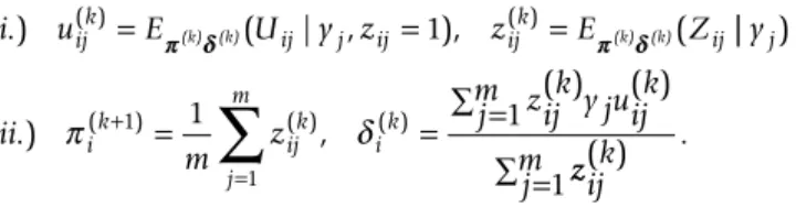
1 1 (10) ˆ . δi zijy juij j m zij j m =∑ = = ∑ 1 1 (11)Equations (6) and (9) – (11) constitute the backbone of the needed closed form EM-algorithm to fit a mixture model like (3) with g + 1 components. Parameter esti-mates are updated according to the scheme
On convergence, the estimated π and δ are used as the parameters of a h(δ) with g + 1 point masses. As discussed above we fix δ0 = 0.
An issue that has received much attention is estimating the proportion of true null hypotheses when many hypothesis tests are performed simultaneously (e.g. [3,22,23]). In the microarray context this amounts to esti-mating the proportion of truly unregulated genes among all genes considered. Referring to (3) we see that this quantity enters our model as π0. To draw on the extensive work on π0-estimation, we suggest using a known con-servative π0-estimate to guide the choice of some model parameters. This is discussed below. In our implementa-tion we use the convex decreasing density estimate pro-posed in [24], but a different estimate may be input. Assessing the appropriate number of components in a mixture model is a difficult problem that is not com-pletely resolved. An often adopted strategy is using meas-ures like the Akaike Information Criterion (AIC) [25] or the Bayesian Information Criterion (BIC) [26]. We find from simulation that, in our setting, these criteria seem to underestimate the needed number of components (refer to the Testing section for some of the simulation results). This is possibly due to the large proportion of unregulated genes often found in microarray data. With relatively few regulated genes, the gain in likelihood from fitting addi-tional components is, for these criteria, not enough to jus-tify the additional parameters used. In our implementation we use g = log2((1 - ) m), where is the above-mentioned estimate. This choice is motivated by experience, but has proven itself adequate in our numerical studies. It also reflects the fact that a single component should provide sufficient explanation for the unregulated genes, while the remaining g components explain the regulated ones. A different g may be specified by users of the sample size method.
A complication that could arise when fitting the mixture
model is that one or more of the , could be
assigned to δ = 0, or very close to it, thus affecting the fit of the central component. To avoid this, we define a small neighbourhood around δ0 = 0 from which all g remaining components are excluded. A δi, i ≠ 0, that tries crossing
into this neighbourhood while fitting the model, is sim-ply halted at the neighbourhood boundary. The boundary is determined by finding the smallest for which it is possible to tell apart the tν(0) distribution from a tν( )
one, based on samples of sizes and (1 - ) m/g,
respectively. The latter sample size assumes regulated genes to be evenly distributed among their components. The samples are taken as evenly spaced points within the 0.05 and 0.95 quantiles of the two distributions. The cri-terion used to check if the two samples originated from the same distribution is a two-sample Kolmogorov-Smir-nov test with a significance level of 0.05. The rationale behind this criteron is that, for the g components associ-ated with regulassoci-ated genes, we only want to allow those that with reasonable certainty can be distinguished from the central component. Again, the used is the estimate discussed above.
Another difficulty related to fitting a mixture model is that the optimal fit is not unique, something which might cause convergence problems. The difficulty is due to the fact that permuting mixture components does not change the likelihood function. In our implementation we do not have any constraints that resolve this problem. We did, however, track the updates of our mixture components in a number of test runs and did not see this problem occur. In summary, our approach provides estimates,
and , of the noncentrality parameters in the data
and a set of weights. Together these quantities make up an estimate of the distribution h(δ). As seen in the section on test-statistics a δ is proportional to the effect size, ξ/σ. No estimates or assumptions are thus made on the numerical size of the means or variances in the data. We only esti-mate a set of mean shift to variance ratios.
Algorithm for estimating sample sizes for FDR control An important issue in experimental design is estimating the sample size required for the experiment to succeed. We now outline how to choose sample sizes that control FDR together with other measures, and how the model discussed above can be used for this purpose.
Table 1 summarizes the possible outcomes of m hypothe-sis tests. All table elements except m are random variables.
i.) u( )ijk =Eππ δδ(k) (k)(Uij|y zj, ij =1), zij( )k =Eππ δδ(k) (k)(Zij|| ) .) , ( ) ( ) ( ) ( ) ( ) y ii m z zijk y juijk j m j ik ijk j m ik π + δ = =
∑
= ∑ = 1 1 1 1 zzijk j m ( ) . = ∑ 1 ˆ π0 πˆ0 { }δi ig=1 δ δ ˆ π0m πˆ0 ˆ π0 { }δi ig=0 { }πi ig=0From Table 1 the much used positive false discovery rate (pFDR) [3] can be defined as E(R0/MR|MR > 0). In [3] it is also proven that, for a given significance region and under assumed independence for the tests, we have
pFDR = Pr(H0 true|H0 rejected), (12)
and that, in terms of p-values p and a chosen p-value cut-off α, (12) can be rewritten as
Equation (13) is important in sample size estimation as it provides the relationship between pFDR, significance region and sample size. Sample size will determine Pr(p
<α) since the shape of the t-distributions depends on n1,
n2. (An explanation is provided at the end this section). The application of (13) to sample size estimation was first discussed by Hu et al. [13].
Using (13), and a fitted mixture model, one can estimate the sample size that achieves a specified α and pFDR. The remaining issue is choosing an appropriate α and pFDR. The pFDR is an easily understood measure, and its size can be set directly by users of the sample size estimation method. How to pick α, on the other hand, is not as clear. One solution to this is to restate (13) as relationships between α, pFDR and other statistical measures. Hu et al. present one such relationship. They suggest picking the α by specifying the expected number of hypotheses to be rejected, E(MR). Their idea is substituting Pr(p <α) = E(MR)/m in (13) to get
In words, instead of specifying an α, one can specify E(MR). This way of obtaining α, however, has a shortcom-ing. It provides little direct information to the user about the experiment's ability to recognize regulated genes. In our view, a more informative way to choose α would be to let the user specify quantities such as average power or the false nondiscovery rate (FNR). We now discuss how this can be accomplished.
Power is defined as the probability of rejecting a hypoth-esis that is false. In the microarray multiple hypothhypoth-esis set-ting, average power controls the proportion of regulated genes that is correctly identified. Setting α through an intuitively appealing measure as average power would thus be helpful. A relationship between α and average power can be found by rewriting the denominator of the right side in (13) as
Pr(p <α) = Pr(p <α|H0 true)π0 + Pr(p <α|H0 false)(1 - π0). Recognizing Pr(p <α|H0 false) as average power, (13) can be inverted to find
Combining (15) and (13) one can now find sample sizes that achieve a specified pFDR and average power, with no need of specifying α.
Another interesting measure to control is the false nondis-covery rate (FNR), the expected proportion of false nega-tives among the hypotheses not rejected. In other words, the FNR controls the proportion of regulated genes erro-neously accepted as unregulated. We use a version of the FNR discussed in [15] called the pFNR = E(A1/MA|MA > 0), which, under the same assumptions as for the pFDR, can be stated as
pFNR = Pr(H0 false|H0 accepted).
Rewriting this probability in terms of pFDR and α yields
Again, specifying a pFNR will correspond to a specific choice of α. The pFNR approach to setting α could be interesting to use. One should note, however, that in the microarray setting this measure can sometimes be hard to apply. The reason is the potentially large MA, due to a high
proportion of unregulated genes. A large MA makes pFNR numerically small, and a reasonable size may be hard to set.
Having chosen a pFDR and α (from average power or
pFNR), we need to find a sample size that solves (13). To do this, we express Pr(p <α) via our mixture model (3) as pFDR( ) Pr( ). α π α α = < 0 p (13) α π = pFDR E 0 ( ) . MR m (14) α π π = − − ⋅ pFDR pFDR average power 1 1 0 0 . (15) α = − −π − − 1 0 1 pFDR pFNR pFDR. (16) Pr( ) ( ; ) , | | p f y h dy y y < = >
∫
α 0 (17)Table 1: Outcomes of m hypothesis tests
H0 accepted H0 rejected Total
H0 true A0 R0 m0
H0 false A1 R1 m1
where y0 is the t-score corresponding to a p-value cutoff α for testing the null hypothesis. Since f(y) is a weighted sum of tν(δ)s, the integrals needed to be taken are simply quantiles of (noncentral) t-distributions. Sample size affects (17) because all tν(δ)s to be integrated are on the
form , with s1(n) and s2(n) dependent
on n1 and n2. (Refer to pdfs of (1) and (2)). If the effect
sizes and the weights were known we
could evaluate (17) for all s1(n), s2(n).
These parameters can, however, be found from the fitted model. To obtain the effect sizes we can equate , where ñ is the sample size used in the fit. The weights are estimated directly. Having expressed Pr(p <α) in terms of sample size we aim to find one that solves (13). This problem can be reformulated as finding the root of the function
For finding the root of S(n) we implement a bisection method.
Testing
To evaluate our approach we implemented the EM-algo-rithm and the sample size estimation method described above. We then ran tests on simulated data sets. For rea-sons discussed above we focused on controlling average power, along with the pFDR, in our sample size estimates. When using simulated data sets it is possible to calculate the true sample size needed to achieve a given combina-tion of pFDR and average power. To evaluate the perform-ance of our method we compared our estimates to the true values. For comparison with existing approaches we also included the estimates made by the methods of Hu et al. [13], Pounds and Cheng [14] and Pawitan et al. [16].
Use of existing methods
In their paper Hu et al. discuss three different mixture models. In our comparison we used their truncated nor-mal model, as this seemed to be the favored one. To pro-duce sample size estimates using this model one needs to input the wanted pFDR and E(MR). As we wished to con-trol pFDR along with average power, we calculated the E(MR) corresponding to each choice of pFDR and average
power as E(MR) = average power·m(1 - π0)/(1 – pFDR). All tests were run with default parameters as found in the
source code. In the implementation of Hu et al., however, three parameters (diffthres, iternum, gridsize) were miss-ing default values. Reasonable choices (0.01,10,100) were kindly provided by the authors.
For the method of Pounds and Cheng one needs to input quantities called anticipated false discovery ratio (aFDR) and anticipated average power. For the estimates pre-sented here we used the corresponding pFDR and average power combination. As Pounds and Cheng work with F-statistics, the t-statistics calculated in our tests were trans-formed accordingly. (If T follows a tνdistribution, then T2 is distributed as F1,ν). In their implementation Pounds and Cheng set an upper limit, nmax, on the sample size estimates, and replace all estimates above nmax with nmax itself. The default value of nmax = 50 was replaced with nmax = 1000 in our tests. The reason for this was that sample size estimates of more than 50 could, and did, occur in the tests. Using a low nmax would then affect the comparison to the other methods. Apart from nmax all tests were run with default parameters as found in the source code.
In [16] Pawitan et al. discuss a method for fitting a mixture model to t-statistics. The fitted model is used to make an estimate of the proportion of unregulated genes, π0. The use of their method for sample size estimation is men-tioned, but is not further explored or tested. The only input needed to fit a model is the number of mixture com-ponents. In our tests, this number was determined using the AIC, as suggested by Pawitan et al. in their paper. In the implementation of Pawitan et al. the assignment of non-central components close to the central one is not restricted. A preliminary test run using their unadjusted model fit showed that sample size estimates were greatly deteriorated by this. In our tests we therefore adjusted their fitted model by collapsing all non-central compo-nents within a given threshold (|δ| < 0.75) into the central one. Our model adjustment corresponds to the π0 -estima-tion procedure used in the implementa-estima-tion of Pawitan et al. For our test runs we used our procedures to produce sample size estimates based on the models fitted by this method.
Test procedure and results
For the test results presented here we used m = 10000 genes, and n1 = n2 = 5 measurements per group. For the proportion of unregulated genes we examined the cases of
π0 = 0.7 and π0 = 0.9.
In a first set of tests we considered sample size estimates in the case of normally distributed measurements and equal variances. In this setting we simulated data with and without a correlation structure. The true distribution of
ts n i i s n 1 1 2 ( )(ξ σ− ( )) {ξ σi i−1}ig=0 { }πi ig=0 δi=ξ σi i−1s n i2( ), =( ,..., )0 g S n i ts n i i s n dy y y i g ( ) ( )( ( )) . | | = − − > =
∫
∑
pFDR π ξ σ π α 1 0 1 2 0 0noncentrality parameters for the m1 = (1 - π0)m regulated genes was generated in the following way: A random sam-ple was drawn from a N(1,0.52) and a N(-1,0.52) distribu-tion. Both samples were of size m1/2, and together they
made up the for the regulated genes in data set.
The measurement variances were set to . The noncentrality parameters of the regulated genes were then calculated as (Refer to discussion of (1)). Based on our experience with microarray data analysis the above choices seem plausible for log-transformed micro-array measurements. Since the true noncentrality parame-ters are all known, the true sample size needed to achieve a particular pFDR and average power can be calculated. Correlation was introduced using a block correlation structure with block size 50. The reasoning behind such a structure was discussed in [27]. All genes, regulated and unregulated, were randomly assigned to their blocks. A correlation matrix for each group was then generated by first sampling random values from a uniform U(-1, 1) dis-tribution into the off-diagonal elements of a symmetric matrix. Then, using the iteration procedure described in [28], we iterated to find the positive semidefinite matrix with unit diagonal that was closest to our randomly gen-erated one.
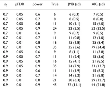
Using the above approach we simulated data. For each test case we generated 50 data sets and made sample size esti-mates based on these. In an initial test run we wanted to evaluate our choice of using a larger number of mixture components, g, than what is suggested by the AIC or BIC criterion. To do so, two models were fitted to each simu-lated data set using our algorithm. One model had our chosen number of mixture components, the other had the number indicated by the AIC. Sample size estimates were then produced for both models. The reason for comparing with the AIC instead of the BIC is that the BIC, in this set-ting, will favor even fewer components than the AIC. In this initial run only uncorrelated data were used. The sam-ple size estimation results are listed in Table 2. The aver-age number of components chosen by the AIC and our method were, respectively, 6.1 and 11.8 for π0 = 0.7 and 5.0 and 10.1 for π0 = 0.9. Based on our findings we con-cluded that there may be an advantage to using more components than suggested by the AIC, and we used this larger number of components in the remaining tests. We then turned our attention to comparing the different approaches to sample size estimation. Uncorrelated and correlated data were generated and sample size estimates were produced using all four methods. The results are
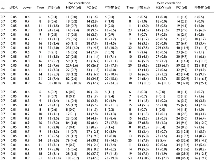
found in the upper half of Table 3. In general it seems that our estimates are close to their true values. Results are slightly better when there is no correlation between genes. As was to be expected, accuracy decreases, and standard deviation increases, with increasing power. This is proba-bly related to the difficult problem of describing the dis-tribution of noncentrality parameters well near the point of no regulation, i.e. close to δ = 0. The estimates of Hu et al. seem largely to be further from the true value than our estimates, and to be more conservative, but have lower standard deviation. The deviation from the true value is particularly high in estimates for high power. The esti-mates of Pounds and Cheng seem to deviate from the true value, be more conservative than our estimates and have higher standard deviation. The conservativeness of the estimates of Pounds and Cheng is seen from their own numerical tests as well, in which the estimated actual power exceeds the desired power. The estimates of Paw-itan et al. appear to be better than those of Hu et al. and Pounds and Cheng, but still seem to be further from the true value than our estimates, and to have higher standard deviation. For high power there is a tendency of underes-timating the needed sample size using this method. Tests with normally distributed measurements were also
run, in which the were drawn from gamma
distri-butions and where variances differed according to the { }ξk km=11 σ2 σ σ 12 22 0 52 = = = . {ξ σk ( ) }k m n n n n − − = + 1 1 2 1 2 1 11 { }ξk km=11
Table 2: Evaluating the number of mixture components. π0 pFDR power True JMB (sd) AIC (sd) 0.7 0.05 0.6 6 6 (0.3) 7 (0.5) 0.7 0.05 0.7 8 8 (0.5) 8 (0.8) 0.7 0.05 0.8 11 10 (1.1) 15 (4.0) 0.7 0.05 0.9 24 22 (2.5) 52 (22.5) 0.7 0.01 0.6 9 9 (0.7) 9 (0.5) 0.7 0.01 0.7 11 11 (0.8) 12 (1.0) 0.7 0.01 0.8 16 15 (1.8) 25 (8.4) 0.7 0.01 0.9 35 35 (3.6) 79 (34.4) 0.9 0.05 0.6 9 8 (1.1) 11 (3.8) 0.9 0.05 0.7 11 11 (2.4) 15 (5.6) 0.9 0.05 0.8 16 15 (4.1) 21 (8.5) 0.9 0.05 0.9 35 24 (7.9) 33 (13.7) 0.9 0.01 0.6 11 11 (1.9) 15 (6.3) 0.9 0.01 0.7 14 14 (3.2) 21 (8.8) 0.9 0.01 0.8 21 20 (6.3) 29 (12.7) 0.9 0.01 0.9 45 32 (11.1) 44 (21.8) True and estimated per group sample sizes for simulated data sets having π0 = 0.7 and π0 = 0.9, and for different pFDR and average power cutoffs. The reported sample size estimate is the average of 50 such estimates rounded off to the nearest integer. The standard deviation (sd) was based on the corresponding 50 data sets. For each data set the estimation method introduced in this paper was used with two different choices for g, the number of mixture components. The JMB column (from the author names) lists the result using a g as discussed in this paper. The AIC column lists the results using the AIC criterion for choosing g.
model discussed below. Results were similar to those dis-cussed above (not shown).
In a second set of tests we wanted to simulate data from a model having the characteristics of a true microarray experiment. We also wanted to see how sample size esti-mates were affected if the assumptions of normality and equal variances did not hold. To accomplish this we based our simulation on the Swirl data set, which is included in the limma software package [29], and on a model for gene expression level measurements discussed by Rocke and Durbin [30]. The model of Rocke and Durbin states that
w = α + µeη+ ∈, (18) where w is the intensity measurement, µ is the expression level, α is the background level and ∈ and η are error terms distributed as N (0, ) and N (0, ) respec-tively. Using the estimation method discussed in their paper we estimated the parameters of (18) for the Swirl
data set. The estimated parameters were, for
the mutant: (394.12, 150.84, 0.18), and for the wild-type: (612.99, 291.40, 0.19). To generate a set of log-ratios rep-resentative of the same data we performed a significance analysis as outlined in the limma user's guide. Using a cut-off level of 0.10 for the FDR-adjusted p-values, we obtained a set of 280 log-ratios for genes likely to be reg-ulated. Log-ratios for the regulated genes in our tests were sampled from this set with replacement. The true expres-sion levels were generated by sampling from the back-ground-corrected mean intensities of the genes in the mutant data set. To simulate microarray data for two con-ditions the following procedure was used: A set of log-ratios, and the true expression levels for one condition, were sampled. The true expression levels for the other condition were then calculated. Using the above-men-tioned model, with their respective sets of parameters, measurements were simulated for both conditions and then log-transformed. To introduce correlation in this set-ting we added a random effect, γ, to the log-transformed measurements for each correlated block of genes. The γ
was drawn from a N (0, ) distribution. The block
size was again assumed to be 50, and the genes were assigned randomly to each block. The true sample size requirements were in this case estimated by repeatedly drawing data sets from the given model and calculating their average power and FDR on a fine grid of cutoff values for the t-statistics. A direct calculation is possible since the regulated genes are known.
After generating a model as described above we again sim-ulated data with and without a correlation structure. For each test setting we sampled 50 data sets and made sam-ple size estimates from the data using all four methods. The results are summarized in the lower half of Table 3. For the methods of Hu et al. and Pounds and Cheng the trend is the same as in the first set of tests. Our method seems to slightly overestimate the needed sample size, while the method of Pawitan et al. now interestingly pro-vides the estimates closest to the true value. The standard deviations for the estimates of Pawitan et al. are still some-what higher than ours.
Note that, since the implementations of Hu et al. and Pounds and Cheng support only sample size estimates based on two-sample t-statistics (1), all tests listed are based on this statistic. Our implementation supports both types, and tests were also run to check the case of one-sample t-statistics (2). The results were similar to those of the two-sample t-statistics (not shown).
Conclusion
We have in this article discussed a mixture model approach to estimating the distribution of noncentrality parameters, and thus effect sizes, among regulated genes in a two-sample comparative microarray study. The model can be fitted to t-statistics calculated from pilot data for the study. We have also illustrated how the model can be used to estimate sample sizes that control the pFDR along with other statistical measures like average power or pFNR. In the microarray setting our results will often also be approximately valid when using the FDR and FNR instead of the pFDR and pFNR. This is due to, referring to Table 1, that one frequently will have Pr(MR) ≈ 1 and Pr(MA) ≈ 1 in this setting. Sample size estimation methods like the one presented are useful in the planning of any large scale microarray experiment.
We examined the accuracy of our sample size estimates by performing a series of numerical studies. The conclusions are that our estimates are reasonably accurate, and have low variance, for moderate cutoffs in the error measures used. For stringent cutoffs we see a larger variance and a somewhat lowered accuracy. Overall our method seems to provide better results than the available sample size esti-mation methods of Hu et al. and Pounds and Cheng. We have also evaluated a method by Pawitan et al. for fitting a mixture model and its use in sample size estimation. The results using the method are good, and our tests suggest that optimizing the method of Pawitan et al. for use in sample size estimation could be interesting.
The decreased accuracy for stringent cutoffs found in the estimates is probably due to the difficult task of describing the distribution of regulated genes well near the point of
σε2 σ
η2
( ,α σ σε, η)
no regulation, that is near δ = 0. It is important that the characterization of such genes is precise, but also that it does not affect the estimated distribution of the unregu-lated genes. Our solution in this article was to introduce a small neighbourhood around δ = 0 in which no other components are fitted. Better ways of differentiating between the two distributions close to 0 could be a subject of further study.
In our tests we also checked how correlation among the genes would affect the sample size estimates. We found that the estimates were only moderately affected. Never-theless, we believe that estimation methods that incorpo-rate correlation among genes is an important topic for future studies.
For the microarray setting the use of a moderated t-statis-tic, as discussed in [31], is often more appropriate than the ordinary t-statistic. For our method to be directly applicable to this type of statistic one would need to know that moderated t-statistics for unregulated genes follow a central t-distribution, and one would need the distribu-tion's degrees of freedom. In [31] this distributional result is shown to hold, with augmented degrees of freedom for the central t-distribution. One would also need to know that moderated t-statistics for a regulated gene, with some given degree of regulation, follow a noncentral t-distribu-tion, and one would need the distribution's degrees of freedom and noncentrality parameter. For this second result we are not aware of any findings. If this second result is shown to hold, then our method can be applied
Table 3: Evaluating sample size estimates from different methods.
No correlation With correlation
π0 pFDR power True JMB (sd) HZW (sd) PC (sd) PMMP (sd) True JMB (sd) HZW (sd) PC (sd) PMMP (sd) 0.7 0.05 0.6 6 6 (0.4) 11 (0.0) 11 (1.6) 6 (0.4) 6 6 (0.5) 11 (0.0) 11 (1.4) 6 (0.5) 0.7 0.05 0.7 8 8 (0.6) 18 (0.2) 14 (2.8) 7 (1.0) 8 8 (1.0) 18 (0.0) 14 (2.3) 7 (0.9) 0.7 0.05 0.8 11 11 (1.5) 39 (0.7) 20 (4.8) 9 (2.5) 11 11 (2.0) 38 (0.5) 19 (4.1) 9 (2.0) 0.7 0.05 0.9 23 24 (3.4) 146 (2.4) 30 (9.5) 13 (6.5) 23 23 (4.5) 145 (1.6) 29 (7.9) 15 (6.8) 0.7 0.01 0.6 9 9 (0.5) 17 (0.5) 16 (2.7) 9 (0.9) 9 9 (0.7) 17 (0.5) 16 (2.4) 8 (0.8) 0.7 0.01 0.7 11 11 (1.1) 28 (0.5) 21 (4.6) 10 (1.7) 11 11 (1.7) 28 (0.5) 21 (3.8) 10 (1.7) 0.7 0.01 0.8 16 16 (2.4) 60 (1.1) 28 (7.9) 13 (4.5) 16 16 (3.3) 60 (0.8) 27 (6.4) 13 (3.4) 0.7 0.01 0.9 34 37 (6.0) 231 (4.2) 42 (14.5) 18 (10.0) 32 36 (7.5) 229 (2.8) 40 (11.9) 22 (11.3) 0.9 0.05 0.6 9 9 (2.1) 16 (0.5) 24 (7.8) 9 (3.9) 8 9 (2.6) 16 (0.5) 23 (6.6) 9 (3.1) 0.9 0.05 0.7 11 11 (3.5) 27 (0.8) 31 (11.4) 11 (7.1) 10 12 (4.1) 27 (0.8) 30 (9.7) 11 (6.6) 0.9 0.05 0.8 16 16 (5.2) 59 (1.7) 41 (16.7) 15 (11.1) 14 16 (5.9) 58 (1.7) 41 (14.4) 15 (11.8) 0.9 0.05 0.9 34 26 (7.6) 227(6.6) 60 (26.8) 21 (17.9) 29 25 (8.5) 225 (6.7) 59 (23.1) 22 (18.8) 0.9 0.01 0.6 11 12 (3.3) 22 (0.7) 33 (11.8) 12 (6.0) 11 12 (4.1) 22 (0.6) 32 (9.9) 12 (4.9) 0.9 0.01 0.7 14 15 (5.3) 38 (1.2) 43 (16.9) 15 (10.4) 13 16 (6.0) 37 (1.2) 42 (14.4) 15 (9.9) 0.9 0.01 0.8 21 21 (7.4) 82 (2.6) 56 (24.3) 20 (15.6) 19 21 (8.4) 81 (2.7) 55 (20.9) 21 (16.8) 0.9 0.01 0.9 46 35 (10.0) 318 (10.0) 79 (37.2) 27 (24.3) 38 33 (11.3) 316 (11.3) 78 (32.0) 29 (25.1) 0.7 0.05 0.6 6 6 (0.2) 6 (0.0) 10 (1.0) 6 (1.1) 6 6 (0.3) 6 (0.0) 10 (1.1) 5 (0.7) 0.7 0.05 0.7 7 8 (0.7) 8 (0.3) 12 (1.7) 8 (2.4) 7 8 (0.7) 8 (0.1) 12 (1.8) 7 (1.6) 0.7 0.05 0.8 9 11 (1.4) 16 (0.4) 16 (2.9) 10 (4.9) 9 11 (1.5) 16 (0.2) 16 (3.2) 10 (3.8) 0.7 0.05 0.9 14 23 (4.1) 56 (1.2) 24 (5.5) 18 (11.3) 15 24 (5.3) 56 (1.0) 25 (6.1) 14 (7.8) 0.7 0.01 0.6 8 8 (0.6) 8 (0.0) 11 (1.7) 8 (2.2) 8 8 (0.7) 8 (0.0) 14 (1.8) 8 (1.0) 0.7 0.01 0.7 10 11 (1.1) 12 0.1) 14 (2.8) 11 (4.3) 10 11 (1.3) 12 (0.1) 18 (2.8) 10 (3.1) 0.7 0.01 0.8 13 16 (2.5) 23 (0.5) 24 (4.6) 15 (8.4) 15 16 (2.5) 23 (0.3) 24 (5.0) 13 (6.4) 0.7 0.01 0.9 26 36 (7.2) 84 (1.8) 35 (8.4) 27 (17.8) 30 37 (8.8) 83 (1.3) 34 (9.4) 20 (12.0) 0.9 0.05 0.6 8 10 (2.0) 7 (0.4) 21 (8.2) 8 (1.6) 8 10 (2.3) 8 (0.4) 24 (8.5) 9 (3.6) 0.9 0.05 0.7 9 13 (3.3) 11 (0.7) 27 (12.1) 10 (3.9) 9 13 (3.4) 12 (0.7) 32 (12.8) 11 (5.7) 0.9 0.05 0.8 12 18 (5.5) 21 (1.2) 37 (19.0) 13 (8.0) 13 19 (5.0) 23 (1.5) 44 (19.7) 14 (8.7) 0.9 0.05 0.9 24 31 (8.5) 76 (4.6) 54 (30.2) 18 (14.5) 25 31 (7.9) 85 5.4) 65 (32.6) 20 (14.5) 0.9 0.01 0.6 11 13 (3.1) 9 (0.5) 29 (12.6) 11 (2.4) 11 13 (3.6) 10 (0.6) 34 (13.2) 12 (5.6) 0.9 0.01 0.7 13 17 (5.0) 16 (0.6) 38 (18.5) 14 (6.2) 14 19 (5.0) 17 (0.8) 45 (19.6) 15 (8.2) 0.9 0.01 0.8 18 25 (8.1) 28 (1.5) 50 (27.2) 17 (11.8) 19 26 (7.1) 31 (1.9) 60 (29.2) 19 (12.3) 0.9 0.01 0.9 51 43 (11.4) 103 (6.2) 72 (42.8) 23 (19.8) 53 43 (10.9) 115 (7.9) 88 (46.3) 26 (19.7) True and estimated per group sample sizes for simulated data sets having π0 = 0.7 and π0 = 0.9, and for different pFDR and average power cutoffs. The reported sample size estimate is the average of 50 such estimates rounded off to nearest integer. The standard deviation (sd) was based on the corresponding 50 data sets. Estimates made using the method discussed in this paper are termed JMB in the table (from the author names), while estimates made by the methods discussed by Hu et al. [13], Pounds and Cheng [14] and Pawitan et al. [16] are termed HZW, PC and PMMP respectively.
to moderated t-statistics as well. Testing the performance of our algorithm with moderated t-statistics, even without the second result, could also be interesting.
In our work we focus on average power as the control measure used along with the pFDR. One should note that having an average power of 0.9 means being able to cor-rectly identify 90% of the regulated genes. In many exper-iments achieving this may not be interesting. One example is studies that aim only at identifying the small set of marker genes that best distinguishes one sample from the other. Other examples are experiments that, when comparing a treated and untreated tissue sample, only are interested in the most heavily affected regulatory pathways. In both these examples a power well below 0.9 could suffice. Our estimates are in this case particularly useful since they seem to be both accurate, and have low variance, for moderate power cutoffs with a low pFDR. Although our main goal in this paper was fitting a model to be used in sample size estimation we would like to emphasize that the fitted model itself does provide some interesting information. One example is a direct estimate of π0, the proportion of unregulated genes, which we often found to be better than the one made by existing methods.
Other subjects for future work include a speed-up of the algorithm. The convergence of a straightforward EM-algo-rithm is known to be rather slow, and methods that improve on it will be implemented. Another issue that may be investigated further is picking the number of model components. As already mentioned, using a few more components than suggested by the traditionally used information criteria would often improve sample size estimates substantially. A different approach might be needed to choose the number of components in this set-ting.
The methods discussed in this article are applicable to any two-sample comparative multiple hypothesis testing situ-ation where t-tests are used, and not only to problems in the microarray setting.
Availability
An implementation of the methods discussed in this paper for the R environment is available from the authors upon request.
Authors' contributions
HM and TSJ developed the statistical algorithms, AMB provided the biological insight. TSJ implemented the methods, ran the tests and drafted the manuscript. HM and AMB revised the manuscript. All authors read and approved the final manuscript.
Acknowledgements
This work was supported by grants NFR 143250/140 and NFR 151991/S10 from the biotechnology and the functional genomics (FUGE) programs of the Norwegian Research Council (AMB, TSJ). Financial support was also given by the cross-disciplinary project "BIOEMIT – Prediction and modifi-cation in functional genomics: combining bioinfomatical, bioethical, biomed-ical, and biotechnlogical research" at the Norwegian University of Science and Technology (HM). The authors would like to thank Mette Langaas for reading the manuscript and making suggestions for improvements. We would also like to thank two anonymous reviewers for their careful reading and helpful advice.
References
1. Callow MJ, Dudoit S, Gong EL, Speed TP, Rubin EM: Microarray Expression Profiling Identifies Genes with Altered Expres-sion in HDL-Deficient Mice. Genome Res 2000, 10:2022-2029. 2. Benjamini Y, Hochberg Y: Controlling the false discovery rate: a
practical and powerful approach to multiple testing. J R Stat Soc Ser B 1995, 57:289-300.
3. Storey JD: A direct approach to false discovery rates. J R Stat Soc Ser B 2002, 64:479-498.
4. Jørstad TS, Langaas M, Bones AM: Understanding sample size: what determines the required number of microarrays for an experiment? Trends Plant Sci 2007, 12:46-50.
5. Gadbury GL, Page GP, Edwards J, Kayo T, Prolla TA, Weindruch R, Permana PA, Mountz JD, Allison DB: Power and sample size esti-mation in high dimensional biology. Stat Methods Med Res 2004, 13:325-338.
6. Müller P, Parmigiani G, Robert C, Rousseau J: Optimal Sample Size for Multiple Testing: the Case of Gene Expression Microarrays. J Am Stat Assoc 2004, 99:990-1001.
7. Jung SH: Sample size for FDR-control in microarray data anal-ysis. Bioinformatics 2005, 21:3097-3104.
8. Li SS, Bigler J, Lampe JW, Potter JD, Feng Z: FDR-controlling test-ing procedures and sample size determination for microar-rays. Stat Med 2005, 24:2267-2280.
9. Pawitan Y, Michiels S, Koscielny S, Gusnanto A, Ploner A: False dis-covery rate, sensitivity and sample size for microarray stud-ies. Bioinformatics 2005, 21:3017-3024.
10. Tibshirani R: A simple method for assessing sample sizes in microarray experiments. BMC Bioinformatics 2006:7.
11. Liu P, Hwang JTG: Quick Calculation for Sample Size while Controlling False Discovery Rate with Application to Micro-array Anaylsis. Bioinformatics 2007, 23:739-746.
12. Ferreira JA, Zwinderman AH: Approximate Power and Sample Size Calculations with the Benjamini-Hochberg Method. Int J Biostat 2007, 2:Article 8.
13. Hu J, Zou F, Wright FA: Practical FDR-based sample size calcu-lations in microarray experiments. Bioinformatics 2005, 21:3264-3272.
14. Pounds S, Cheng C: Sample Size Determination for the False Discovery Rate. Bioinformatics 2005, 21:4263-4271.
15. Storey JD: The Positive False Discovery Rate: A Bayesian Interpretation and the q-value. Ann Stat 2003, 31:2013-2035. 16. Pawitan Y, Murthy KRK, Michiels S, Ploner A: Bias in the
estima-tion of the false discovery rate in microarray studies. Bioinfor-matics 2005, 21:3865-3872.
17. Lindsay BG: The Geometry of Mixture Likelihoods: A General Theory. Ann Stat 1983, 11:86-94.
18. Dempster AP, Laird NM, Rubin DB: Maximum Likelihood from Incomplete Data via the EM Algorithm. J R Stat Soc Ser B 1977, 39:1-38.
19. Johnson NL, Kotz S, Balakrishnan N: Continuous Univariate Distributions Volume 2. second edition. John Wiley and Sons, Inc; 1995.
20. McLachlan G, Peel D: Finite Mixture Models John Wiley and Sons, Inc; 2000.
21. Jeffreys H, Jeffreys BS: Methods of Mathematical Physics third edition. Cambridge University Press; 1972.
22. Schweder T, Spjøtvoll E: Plots of p-values to evaluate many tests simultaneously. Biometrika 1982, 69:493-502.
23. Allison DB, Gadbury GL, Heo M, Fernandez JR, Lee CK, Prolla TA, Weindruch R: A mixture model approach for the analysis of
Publish with BioMed Central and every scientist can read your work free of charge "BioMed Central will be the most significant development for disseminating the results of biomedical researc h in our lifetime."
Sir Paul Nurse, Cancer Research UK Your research papers will be:
available free of charge to the entire biomedical community peer reviewed and published immediately upon acceptance cited in PubMed and archived on PubMed Central yours — you keep the copyright
Submit your manuscript here:
http://www.biomedcentral.com/info/publishing_adv.asp
BioMedcentral
microarray gene expression data. Comput Stat Data An 2002, 39:1-20.
24. Langaas M, Lindqvist BH, Ferkingstad E: Estimating the proportion of true null hypotheses, with application to DNA microarray data. J R Stat Soc Ser B 2005, 67:555-572.
25. Akaike H: Information theory and an extension of the maxi-mum likelihood principle. Second International Symposium on Infor-mation Theory 1973:267-281.
26. Schwarz G: Estimating the Dimension of a Model. Ann Stat 1978, 6:461-464.
27. Storey JD: Invited comment on 'Resampling-based multiple testing for DNA microarray data analysis' by Ge, Dudoit, and Speed. Test 2003, 12:1-77.
28. Higham NJ: Computing the nearest correlation matrix – a problem from finance. IMA J Numer Anal 2002, 22:329-343. 29. Smyth GK: Limma: linear models for microarray data. In
Bio-informatics and Computational Biology Solutions using R and Bioconductor Edited by: Gentleman R, Carey V, Dudoit S, Irizarry R, Huber W. Springer, New York; 2005:397-420.
30. Rocke DM, Durbin B: A Model for Measurement Error for Gene Expression Arrays. J Comput Biol 2001, 8:557-569. 31. Smyth GK: Linear Models and Empirical Bayes Methods for
Assessing Differential Expression in Microarray Experi-ments. Stat Appl Genet Mol Biol 2004, 3:Article 3.