Differential expression analysis for sequence count data

Differential expression analysis for sequence count data

Simon Anders

, Wolfgang Huber

European Molecular Biology Laboratory (EMBL), Heidelberg, Germany

7 Jan 2010

Abstract

Motivation: High throughput nucleotide sequenc-ing provides quantitative readouts in assays for RNA expression (RNA-Seq), protein-DNA binding (ChIP-Seq), cell counting. Statistical inference of differ-ential signal in these data needs to take into ac-count their natural variability throughout the dynamic range. When the number of replicates is small, error modeling is needed to achieve statistical power. Results: We propose an error model that uses the negative binomial distribution, with variance and mean linked by local regression, to model the null distribution of the count data. The method controls type I error and provides good detection power. Availability: A free open-source R software pack-age, called DESeq, is available from http://www-huber.embl.de/users/anders/DESeq (and will be avail-able from the Bioconductor project).

Contact: [email protected]

1

Introduction

High-throughput sequencing of DNA fragments of-fers unprecedented opportunities for the monitoring of RNA abundance and of proteDNA binding, in-cluding the possibility to discover novel sequence vari-ants and to dissect allele-specific effects and genetic variation. There is a range of technologies; a com-mon feature between them is that they produce large amounts of sequence reads sampled from a prepara-tion of DNA fragments that reflects, e.g., a biological system’s repertoire of RNA molecules (RNA-Seq, Na-galakshmi et al. (2008); Mortazavi et al. (2008)) or the DNA or RNA interaction regions of nucleotide binding molecules (ChIP-Seq, Robertson et al. (2007); HITS-CLIP, Licatalosi et al. (2008)). Typically, these reads are classified based on their mapping to a common region of the target genome, where each class repre-sents a target transcript, in the case of RNA-Seq, or a binding region, in the case of ChIP-Seq. An

im-∗_{[email protected]}

portant summary statistic is the number of reads in a class; for RNA-Seq, this read count has been found to be (to good approximation) linearly related to the abundance of the target transcript (Mortazavi et al., 2008). Interest lies in comparing read counts between different biological conditions or between different ge-netic variants. In the simplest case, the comparison is done separately, class by class. We will use the term

gene synonymously toclass, even though a class may also refer to, e.g., a transcription factor binding site, or even a barcode (Smith et al., 2009).

We would like to use statistical testing to decide whether, for a given gene, an observed difference in read counts is significant, i.e., whether it is greater than what would be expected just due to natural ran-dom variation.

If reads are independently sampled from a popu-lation with given, fixed fractions of genes, the read counts follow a multinomial distribution, which can be approximated by Poisson distributions. Consequently, Poisson distributions have been used to test for dif-ferential expression (Marioni et al., 2008; Wang et al., 2010). The single parameter of a Poisson distribu-tion is determined by its mean, and its variance and all other properties follow from that; especially, the variance is equal to the mean. However, it has been noted (Robinson and Smyth, 2007; Nagalakshmi et al., 2008) that the assumption of Poisson distribution for the read counts is too tight, i. e., it predicts smaller variations than what is seen in the data. The resulting statistical test does therefore not control the type I er-ror (the probability of false discoveries) as advertised. We show instances for that in Section 5.1.

To address this so-called overdispersion problem, it has been proposed to model count data with neg-ative binomial (NB) distributions (Whitaker, 1914), and this approach is used in the edgeR package for analysis of SAGE and RNA-Seq (Robinson and Smyth, 2007; Robinson et al., 2010). The NB distributions are a family with two parameters, which are uniquely determined by mean µand variance v. However, the number of replicates in datasets of interest is often too small to estimate both of those two parameters, mean

and variance, reliably for each gene. ForedgeR, Robin-son and Smyth (2008) proposed to assume that mean and variance are related byv=µ+αµ2_{, with a single}

proportionality constantα that is the same through-out the experiment and that can be readily estimated from the data. Hence, only one parameter needs to be estimated for each gene, allowing application to exper-iments with small numbers of replicates.

In this paper, we extend this model by allowing more general, data-driven relationships of variance and mean, provide an effective algorithm for fitting the model to data, and show that it provides better fits. As a result, more balanced selection of differentially expressed genes throughout the dynamic range of the data and higher power for the detection of differential abundance can be obtained. The method is applicable to a wide range of experimental designs and questions. We will first specify our model and explain how to fit its parameters (Section 2) and then how to test for dif-ferential expression (Section 3). We demonstrate the method by applying it to three data sets (Section 4) and discuss how it compares to alternative approaches (Section 5). Finally, we present the R implementation of the method, calledDESeq (Section 6).

2

Model

2.1

Description

We assume that the number of reads in samplejthat are assigned to gene i can be modeled by a negative binomial (NB) distribution,

Kij∼NB(µij, σij2), (1)

which has two parameters, the meanµij and the

vari-ance σ2

ij. The read counts Kij are non-negative

inte-gers. The probabilities of the distribution are given in Supplementary Note A. This family of distributions is commonly used to model count data when overdisper-sion is present (Cameron and Trivedi, 1998).

In practice, we do not know the parametersµij and

σ_ij2, and we need to fit them from the data. Typically, the number of replicates is small, and further modeling assumptions need to be made in order to obtain useful estimates. In this paper, we develop a method that is based on the following three assumptions:

First, the mean parameterµij, that is, the

expecta-tion value of the observed counts for geneiin sample

j, is the product of a condition-dependent per-gene valueqi,ρ(j) (whereρ(j) is the experimental condition

of samplej) and a library size parametersj,

µij=qi,ρ(j)sj. (2)

qi,ρ(j) is proportional to the expectation value of the

true (but unknown) concentration of fragments from gene i under condition ρ(j). The library size param-eter sj is proportional to the coverage, or sampling

depth, of library j, and we will use the term common scale for quantities, such as qi,ρ(j), that are adjusted

for coverage by dividing by sj.

Second, the variance σ2

ij is the sum of ashot noise

term and araw variance term,

σ_ij2 = µij |{z} shot noise + s2_jvi,ρ(j) | {z } raw variance (3)

Third, the per-gene raw variance parametervi,ρ(j)is

a smooth functionvρof the per-gene abundanceqi,ρ(j),

vi,ρ(j)=vρ(qi,ρ(j)). (4)

The decomposition of the variance in Equation (3) is motivated by the following hierarchical model. We as-sume that the actual concentration of fragments from gene i in sample j is proportional to a random vari-ableRij, such that the rate that fragments from gene

i are actually sequenced issjrij. For each geneiand

all samples j of condition ρ, the Rij are i.i.d. with

meanqiρand varianceviρ. Thus, the count valueKij,

conditioned on Rij =rij, is Poisson distributed with

rate sjrij. If the higher moments of the distribution

of Rij are modeled according to a gamma

distribu-tion, the marginal distribution of Kij is NB (see e.g.

Cameron and Trivedi (1998, Sec. 4.2.2)) with mean

µij and variance as given in Equation (3).

The model could be refined by adding further pa-rameters. For example, when the experimental pro-tocols involves DNA fragmentation, one may want to divide the mean qiρ in Equation (4) by the feature

length.

2.2

Fitting

We now describe how the model can be fit to data. The data are ann×mtable of counts,kij, wherei=

1, . . . , n indexes the genes, and j = 1, . . . , m indexes the samples. The model has three sets of parameters: 1. mlibrary size parameterssj; the expectation

val-ues of all counts from sample j are proportional to sj.

2. for each experimental condition ρ, n gene abun-dance parameters qiρ; they reflect the expected

abundance of fragments from geneiunder condi-tion ρ, i.e., expectation values of counts for gene

i are proportional toqiρ.

3. The smooth functionsvρ:R+→R+; they model

the dependence of the raw varianceviρon the

ex-pected meanqiρ.

To estimate the size parameters, we use ˆ sj= median i kij (Πm ν=1kiν) 1/m. (5)

The denominator of this expression can be interpreted as a pseudo-reference sample obtained by taking the geometric mean across samples. Each library size pa-rameter estimate ˆsjis then computed as the median of

the ratios of the j-th sample’s counts to those of the pseudo-reference. In many cases, the values ˆsj will

be proportional to, and thus equivalent to, the sums

P

ikij. However, it is not uncommon for the sums to

be dominated by the counts for a few, highly abundant genes. In such cases, the estimator (5) will be more ro-bust, and will produce a better library size adjustment for the majority of genes.

To estimate qiρ, we use the average of the counts

from the samples j corresponding to condition ρ, transformed to the common scale:

ˆ qiρ = 1 mρ X j:ρj=ρ kij ˆ sj , (6)

where mρ is the number of replicates of condition ρ

and the sum runs over these replicates.

To estimate the functionsvρ, we first calculate

sam-ple variances on the common scale

wiρ= 1 mρ−1 X j:ρ(j)=ρ _k ij ˆ sj −qˆiρ 2 (7) and define ziρ = ˆ qiρ mρ X j:ρ(j)=ρ 1 ˆ sj . (8)

In Supplementary Note B, we show thatwiρ−ziρ is

an unbiased estimator for the raw variance parameter

viρ of Equation (3).

However, for small numbers of replicates,mρ, as is

typically the case in applications, the values wiρ are

highly variable, and wiρ−ziρ would not be a useful

variance estimator for statistical inference. Instead, we use local regression (Loader, 1999) on the graph (ˆqiρ, wiρ) to obtain a smooth functionwρ(q), with

ˆ

vρ(ˆqiρ) =wρ(ˆqiρ)−ziρ (9)

as our estimate for the raw variance.

Some attention is needed to avoid estimation biases in the local regression. wiρis a sum of squared random

variables, and the residualswiρ−w(ˆqiρ) do not follow a

normal distribution. Following McCullagh and Nelder (1989, Ch. 8) and Loader (1999, Section 9.1.2), we use a generalised linear model of the gamma family for the local regression, using the implementation in thelocfit

package (Loader, 2007).

3

Testing for differential

expres-sion

Suppose that we have mA replicate samples for

bio-logical condition A and mB samples for condition B.

For each genei, we would like to weigh the evidence in the data for or against differential abundance of that gene between the two conditions. In particular, we would like to test the null hypothesisqiA=qiB, where

qiA is the gene abundance parameter for the samples

of condition A, and qiB for condition B. To this end,

we define, as test statistic, the total counts in each condition, KiA= X j:ρ(j)=A Kij KiB = X j:ρ(j)=B Kij, (10)

and their overall sum KiS = KiA+KiB. From the

error model of Section 2, we show below that we can compute the probabilities of the events KiA =a and

KiB =b for any pair of numbersa andb. We denote

this probability by p(a, b). The p-value of a pair of observed count sums (kiA, kiB) is then the sum of all

probabilities less or equal top(kiA, kiB), given that the

overall sum is kiS: pi= P a+b=k_iS p(a,b)≤p(k_iA, k_iB) p(a, b) P a+b=k_iS p(a, b) (11)

The variablesaandbin the above sums take the values 0, . . . , kiS. The approach presented so far follows that

of Robinson and Smyth (2008) and is analogous to that taken by other conditioned tests, such as Fisher’s exact test. (See Agresti (2002, Ch. 2) for a discussion of the merits of conditioning in tests.)

Computation of p(a, b). First, assume that, under the null hypothesis, counts from differ-ent samples are independdiffer-ent. Then, p(a, b) = Pr (KiA=a) Pr (KiB=b). The problem thus is

com-puting the probability of the eventKiA=a, and,

anal-ogously, of KiB=b. The random variable KiA is the

sum ofmA NB-distributed random variables. We

ap-proximate its distribution by a NB distribution whose parameters we obtain from those of the Kij. To this

end, we first compute the pooled mean estimate from the counts of both conditions,

ˆ

qi0=

X

j:ρ(j)∈{A,B}

kij/sj, (12)

which accounts for the fact that the null hypothesis stipulates that qiA = qiB. The summed mean and

variance for condition A is ˆ µiA = X j∈A sjqˆi0, (13) ˆ σ_i2_A = X j∈A ˆ sjqˆi0+ ˆs2jvˆA(ˆqi0), (14)

Supplementary Note C describes how the distribution parameters of the NB forKiAcan be determined from

ˆ

µiAand ˆσi2A. (We do not use the moments directly but

instead perform an additional bias-correcting step.) The parameters of KiB are estimated analogously.

Supplementary Note D explains how we evaluate the sums in Equation (11).

4

Applications

4.1

Data sets

We demonstrate the application of our method, which we callDESeq, on the following data sets.

Tag-Seq of neural stem cells. Engstr¨om et al. (2010) performed Tag-Seq (Morrissy et al., 2009) for tissue cultures of neural cells, including two from glioblastoma-derived neural stem-cells (condi-tion GNS; samples G144, G166) and two from non-cancerous neural stem cells (condition NS; samples NS123, NS345). The number of reads obtained from each library varied from 7.6 millions to 13.6 millions. A good fraction of these (depending on the sample, from 32% to 53%) could be unambiguously assigned to an-notated genes, and Engstr¨om et al. (2010) et al. sum-marised the data in a table of counts with six columns for the six samples and 18,760 rows, one for each gene. RNA-Seq of yeast. Nagalakshmi et al. (2008) per-formed RNA-Seq on replicates of yeast cultures. They tested two library preparation protocols,dT andRH, and obtained three sequencing runs for each protocol, such that for the first run of each protocol, they had one further technical replicate (same culture, repli-cated library preparation) and one further biological replicate (different culture).

ChIP-Seq in humans. This dataset contains four replicates each from a ChIP-Seq experiment studying polymerase-II occupancy in two different human indi-viduals.

4.2

Variance estimation

We start by demonstrating the variance estimation. Figure 1a shows the sample variances wiρ

(Equa-tion (7)) plotted against the means ˆqiρ (Equation (6))

p value P ercent of T otal 0 10 20 30 0.0 0.2 0.4 0.6 0.8 1.0

DESeq lower half DESeq upper half

0.0 0.2 0.4 0.6 0.8 1.0

DESeq all edgeR lower half

0.0 0.2 0.4 0.6 0.8 1.0

edgeR upper half

0 10 20 30 edgeR all

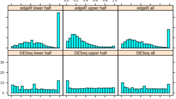
Figure 3: Type-I error control. The histograms showp val-ues from a comparison of oneGNSreplicate with another one. Between replicates, no genes are truly differentially expressed, and the distribution of p-values is expected to be uniform in the interval [0,1]. Top row shows results foredgeR, lower row forDESeq. Left and middle column show the distributions sepa-rately for genes below and above the median mean, right column for all genes. DESeq’s more flexible variance estimation leads to approximately uniformpvalue distributions independent of the mean level, whereas those obtained withedgeRshow intensity dependent trends.

for the condition ρ = GNS in the neural stem cells data. Also shown is the local regression fit wρ(q) and

the shot noise ˆsjqˆiρ. In Figure 1b, we plotted the

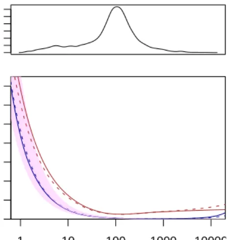
squared coefficient of variation (SCV), i.e. the ratio of the variance to the mean squared. In this plot, the distance between the orange and the purple line is the SCV of the noise due to biological sampling (cf. Equa-tion (3)).

The many points in Figure 1a that lie far above the fitted orange curve may let the fit of the local regres-sion appear poor. However, a strong skew of the resid-ual distribution is to be expected. See Supplementary Note E for details and a discussion of diagnostics suit-able to verify the fit.

4.3

Testing

In order to verify control of type-I error, we contrasted one GNS replicate against another replicate of the same condition, using for both samples the variance function estimated for condition GNS. In this case, we expect to find uniformly distributedpvalues. Figure 3 (lower row) shows this to be the case.

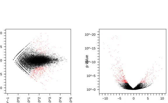
Next, we contrasted the two GNS samples against the two NS samples. Using the procedure described in Section 3, we computed a p value for each gene. Figure 2 shows the obtained fold changes and p val-ues. 10% of the p values are below 5%. Adjust-ment for multiple-testing with the false discovery rate (FDR) controlling procedure of Benjamini and Hochberg (1995) yielded significant differential

mean v ar iance 10^−4 10^−2 10^0 10^2 10^4 10^6 10^8 10^0 10^1 10^2 10^3 10^4 mean squared coefficient of v ar iation 0.2 0.4 0.6 0.8 1.0 1.2 1.4 1.6 1.8 10^0 10^1 10^2 10^3 10^4

Figure 1: Dependence of the variance on the mean for the twoGNSsamples from the neural stem cells data. (a) The scatter plot shows the common-scale sample variances (Equation (7)) plotted against the common-scale means (Equation (6)). The orange line is the fitw(q). The purple lines show the variance implied by the Poisson distribution for each of the twoGNSsamples, i.e., ˆsjqˆi,GNS.

The dashed orange line is the variance estimate used byedgeR. (b) Same data as in (a), with they-axis rescaled to show the squared coefficient of variation (SCV), i.e. all quantities are divided by the square of the mean. The solid orange line is computed using the bias correction described in Supplementary Note C.

mean log2 f old change −10 −5 0 5 10

10^−1 10^0 10^1 10^2 10^3 10^4 10^5 log2 fold change

p v alue 10^−0 10^−5 10^−10 10^−15 10^−20 −10 −5 0 5 10

Figure 2: Testing for differential expression between conditionsGNS andNS. (a) Scatter plot of log₂ fold changes versus mean. The red colour marks genes detected as differentially expressed at 10% false discovery rate when the Benjamini-Hochberg multiple testing adjustment is used. (b) Vulcano plot.

−1 0 1 2 3 4 5 0.00 0.02 0.04 0.06 log10 mean density x7

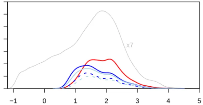
Figure 4: The density of common-scale mean valuesqifor all genes (grey line, scaled down by a factor of 7, for the hits re-ported by DESeq (red line) and by edgeR with four different settings (light blue, using read count sum for library size ad-justment; dark blue, using Equation (5); solid, with common dispersion; dashed, with tagwise dispersion.)

sion at a 10% FDR level for a set of 680 genes (of 18,323). These are marked in red in the figure.

Figure 2 demonstrates that the power to detect dif-ferential expression depends on overall counts: below a common scale mean of∼10, no detection is possible, and as the mean grows, smaller fold changes become detectable.

4.4

Comparison with edgeR

We also compared the threeGB samples with the two

NS samples usingedgeR (version 1.5.4; Robinson and Smyth (2007, 2008); Robinson et al. (2010)). While

DESeq reports 680 genes at Benjamini-Hochberg ad-justed FDR of 10%,edgeR finds 452 genes when used incommon dispersionmode and 256 in thetagwise dis-persionmode. These numbers foredgeRwere obtained when supplying it with total read counts as library size parameters, as recommended in the documenta-tion; whenDESeq’s estimates, as in Equation (5), were used, we obtained 525 and 316 genes, respectively. 84% to 96% of edgeR’s genes were also reported by

DESeq, which is consistent with an FDR of 10%. The difference between the results ofedgeRand DE-Seq does not merely lie in the number of genes, but also in their properties. As can be seen from Fig-ure 4, the gene lists have different distributions along the abundance scale. While –for these data– edgeR’s hits tend to concentrate at lower abundance, the hits fromDESeqare more evenly distributed along the

dy-69

418

202

15,529

Figure 5: Calling differential expression without replicates: The red set in this Venn diagram represents the genes that were found to show differential expression significant at 10% FDR when comparing threeGNSsamples with the twoNS samples. When using only one sample of each type, the genes represented by the blue set are found.

namic range, once the mean is above ∼ 10. edgeR’s bias towards lower abundance genes is likely not a re-flection of biology, but rather an artifact of its error model: edgeR estimates a common dispersion of 0.56 (0.60 with read count sum). The dashed orange line in Figure 1a and b shows the variance implied by a raw SCV of this value. As one can see, it is lower than DE-Seq’s estimate (solid orange line) for the lower part of the the dynamic range, and higher in the upper range. Hence, edgeR calls more hits among genes with low counts and is conservative for genes with high counts. This matches the observation from Figure 4. On av-erage, over the whole dynamic range, FDR control is of course maintained, albeit at the cost of detection power.

A similar effect can be observed in the comparison of the two GNS replicates against each other. As can be seen in Figure 3, there are either too many high or too many low pvalues, depending on the range of mean values.

4.5

Working without replicates

DESeq allows analysis of experiments with no biologi-cal replicates in one or even in both of the conditions. While one may not want to draw strong conclusions from such an analysis, it may still be useful for explo-ration and hypothesis geneexplo-ration.

If replicates are available only for one of the condi-tions, one may assume that the variance-mean depen-dence estimated from the data for that condition holds as well for the unreplicated one.

If neither condition has replicates, one can still per-form an analysis based on the assumption that for most genes, there is no true differential abundance, and that a valid mean-variance relationship can be es-timated from treating the two samples as if they were replicates. A minority of differentially abundant genes will act as outliers, however, they will not have a se-vere impact on the gamma-family GLM fit, as the gamma distribution for low values of the shape

GliNS1 G144 CB660 CB541 G166 G179 GNS (L) GNS NS NS GNS (*) GNS (*) 0 50 150 250 Value Color Key

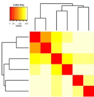
Figure 6: Sample clustering for the data of Engstr¨om et al. (2010). A common variance function was estimated for all sam-ples and used to apply a variance-stabilizing transformation. The heatmap shows a false colour representation of the Eu-clidean distance matrix, and the dendrogram represents a hi-erarchical clustering. The twoGNS samples derived from the same patient (marked with “(*)”) show the highest degree of similarity. The two otherGNSsamples (including the one with atypically large cells, marked “(L)”) are as dissimilar from the former as the twoNSsamples.

rameter (m−1)/2 has a heavy right-hand tail. Some overestimation of the variance may be expected, which will make that approach conservative.

We performed such an analysis by restricting the neural stem cells data to only two samples, one from the GNS and one from the NS condition. The esti-mated variance function is, as expected, above the two functions estimated from theGNS andNS replicates. Using it to test for differential abundance still finds a number of hits at 10% FDR, as can be seen from the Venn diagram in Figure 5, and these hits have good overlap with those found from the more reliable anal-ysis with all available samples.

4.6

Variance-stabilizing

transforma-tion

Given a variance-mean dependence, a variance-stabilizing transformation (VST) is a bijection such that for the transformed values, the variance is (ap-proximately) independent of the mean. Using the variance-mean dependence estimated by DESeq, the functionv(q), a VST is given by

τ(κ) =

Z κ _dq

p

v(q). (15) Using the transformationτon the common-scale count data, kij/sj, yields new data values whose variance

is approximately the same throughout the dynamic range.

One application of VST is sample clustering, as in Figure 6; such an approach is more straightforward than, say, defining a suitable distance metric on the

data P ercent of T otal 0 20 40 60 0.0 0.2 0.4 0.6 0.8 1.0 D: A1 vs A2 D: B1 vs B2 0.0 0.2 0.4 0.6 0.8 1.0 D: A1 vs B1 D: A1,A2 vs B1,B2 P: A1 vs A2 0.0 0.2 0.4 0.6 0.8 1.0 P: B1 vs B2 P: A1 vs B1 0.0 0.2 0.4 0.6 0.8 1.0 0 20 40 60 P: A1,A2 vs B1,B2

Figure 7: Application to ChIP-Seq data. Shown arepvalue histograms resulting from comparisons of Pol-II ChIP-Seq data between replicates of the same individual (first and second umn) and between two different individuals (third and forth col-umn). The upper row corresponds to an analysis based on Pois-son GLMs (“P”), the bottom row to analysis withDESeq(“D”). In the first column, two replicates from individual A (replicate setA1) are compared against two further replicates from the same individual (A2). As expected, thepvalue histograms are approximately flat, indicating no significant differences. In the second column, two replicates from individual B (B1) are com-pared against two further replicates from the same individual (B2). While no significant differences are expected, the Poisson GLM analysis finds an enrichment of smallp values; this is a reflection of overdispersion in the data, that is, the variance in the data is larger than what the Poisson GLM assumes (see also Section 5.1 ). The third column compares two replicates from individual A (A1) against two from individual B (B1). True binding differences are expected, and both methods result in an excess of smallpvalues. The forth column shows the com-parison of four replicates of individual A (A1 combined with

A2) against four replicates of individual B (B1,B2); increased sample size leads to higher detection power.

untransformed count data, whose choice is not obvi-ous, and may not be easy to combine with available clustering or classification algorithms. Another use is the computation of more complex contrasts, such as in-teractions between experimental factors or regression on continuous-valued variables, and analysing the ef-fects as if the data were homoskedastic. However, the power of such an approach would be lower than in the NB-based approach of Section 3, since it ignores the discreteness and skewedness of the count data.

4.7

ChIP-Seq

An application ofDESeqto ChIP-Seq data is shown in Figure 7. For two human individuals (“A” and “B”), four replicates of ChIP-Seq for polymerase-II had been done. Using a pre-compiled list of binding regions, a table of count data can be obtained by counting the number of reads aligned to each binding region (which

now take the place of genes).

In analysing this table, type-I error control was maintained by DESeq: the lower left two panels of Figure 7 show approximately uniform p value his-tograms for comparisons within the same individual, and no binding region was significant at 10% FDR using Benjamini-Hochberg adjustment. Differential binding was found, however, when contrasting the two individuals, with 6,450 binding regions significant when only two replicates each were used and 9,415 when four replicates were used.

However, if one assumed the read counts to follow Poisson distributions, a standard approach would be to perform count regression, i.e., to use a generalized linear model (GLM) of the Poisson family (Cameron and Trivedi, 1998). The upper row of Figure 7 shows that for this approach an enrichment of smallpvalues even for comparisons within the same individual, indi-cating that the variance is underestimated, and literal use of thepvalues would hence lead to anticonserva-tive (overly optimistic) calling of differential binding regions.

5

Discussion

Why is it necessary to develop new statistical method-ology for sequence count data? If large numbers of replicates were available, questions of data distribu-tion could be avoided by using non-parametric meth-ods, such as Wilcoxon and Kruskal-Wallis tests. How-ever, it is desirable (and possible) to consider exper-iments with smaller numbers of replicates per condi-tion. In order to compare an observed difference with the to be expected random variation, we can employ two sources of information on the size and nature of random variation: first, we can use distribution fam-ilies, such as normal, Poisson and negative binomial distributions, in order to determine the higher mo-ments, and hence the tail behavior, of statistics for differential abundance, based on observed low order moments such as mean and variance. Second, we can share information between genes, based on the notion that data from different genes follow similar patterns of variability. Here, we have described an instance of such an approach, and we will now discuss the choices we have made.

5.1

Distributional family

While for large counts, the normal distributions might provide a good approximation of between replicate variability, this is not the case for lower count values, whose discreteness and skewness mean that probabil-ity estimates computed from a normal approximation

0.00 0.25 densqNaga$x density 1 10 100 1000 10000 0.0 0.4 0.8 1.2 mean squared coefficient of v ar iation

Figure 8: Noise estimates for the data of Nagalakshmi et al. (2008). The data allow assessment of technical variability (be-tween library preparations from aliquots of the same yeast culture) and biological variability (between two independently grown cultures). The blue curves depict the squared coefficient of variation at the common scale, wρ(q)/q2 _{(see Equation (9))}

for technical replicates, the red curves for biological replicates (solid lines,dTdata set, dashed lines,RH data set). The data density is shown by the black curve in the top panel. The purple area marks the range of the shot noise for the range of library sizes in the data set. One can see that the noise between techni-cal replicates follows closely the shot noise limit, while the noise between biological replicates exceeds shot noise already for low count values.

would be inadequate.

For the Poisson approximation, a key paper is the work by Marioni et al. (2008), who studied the techni-cal reproducibility of RNA-Seq. They extracted total RNA from two tissue samples, one from the liver and one from the kidneys of the same individuum. From each RNA sample they took seven aliquots, prepared a library from each aliquot according to the protocol recommended by Illumina and sampled each library on one lane of a Solexa genome analyzer. For each gene, they then calculated the variance of the seven counts from the same tissue sample and found very good agreement with the variance predicted by a Pois-son model. In line with our arguments in Section 2, Poisson shot noise is the minimum amount of variation to expect in a counting process. Thus, Marioni et al. (2008) concluded that the technical reproducibility of RNA-Seq is excellent, and that the variation between technical replicates is close to the shot noise limit.

From this vantage point, Marioni et al. (2008) sug-gested to use the Poisson model (and Fisher’s exact test, or a likelihood ratio test as an approximation to it) to test whether a gene is differentially expressed be-tween their two samples. It is now vital to notice that

a rejection from such a test only informs us that the difference between the average counts in the two sam-ples is larger than one would expect betweentechnical

replicates. Hence, we do not know whether this differ-ence is due to the different tissue type, kidney instead of liver, or whether a difference of the same magnitude could have been found as well if one had compared two samples from different parts of the same liver, or from livers of two individuals.

Figure 1 shows that shot noise (purple region) is only dominant for very low count values, while already for moderate counts, the effect of the biological varia-tion between samples exceeds the shot noise by many orders of magnitude. This is confirmed by compar-ison of technical with biological replicates (Nagalak-shmi et al., 2008). In Figure 8, we used DESeq to obtain variance estimates for the data of Nagalakshmi et al. (2008). The analysis indicates that the difference between technical replicates barely exceeds shot noise level, while biological replicates differ much more.

Tests for differential abundance that are based on a Poisson model, such as proposed by Jiang and Wong (2009) or Wang et al. (2010) should thus be interpreted with caution, as they will tend to underestimate the effect of biological variability.

Consequently, it is preferable to use a model that allows for overdispersion. While for the Poisson distri-butions, variance and mean are equal, the negative bi-nomial distributions are a generalisation that allow for the variance to be larger. The most advanced of the published methods using this family of distributions is likely edgeR (Robinson and Smyth, 2007). DESeq

owes its basic idea to a good part toedgeR, but differs in several aspects.

5.2

Sharing of information between

genes

First, we discovered that the use of total read counts as estimates of sequencing depth, and hence for the ad-justment of observed counts between samples (as rec-ommended by Robinson and Smyth (2007) and other authors) may result in high apparent differences be-tween replicates, and hence in poor power to detect true differences. DESeq uses the more robust size es-timate Equation (5); in fact,edgeR’s power increases when it is supplied with those size estimates instead.

For small numbers of replicates such as often en-countered in practice, it is not possible to obtain si-multaneously reliable estimates of the variance and mean parameters of the NB distribution. edgeR ad-dresses this problem by estimating a single common dispersion parameter. In our method, we make use of the possibility to estimate a more flexible,

mean-dependent local regression. The amount of data avail-able in typical experiments is large enough to allow for sufficiently precise local estimation of the dispersion. Over the large dynamic range that is typical for RNA-Seq, the raw SCV often appears to change noticeably, and taking this into account allows DESeq to avoid bias towards certain areas of the dynamic range in its differential-expression calls (see Figures 3 and 4).

This flexibility is the most substantial difference be-tween DESeq and edgeR, as simulations show that

edgeR and DESeq perform comparably if provided with artificial data with constant SCV (Supplementary Note F). edgeR attempts to make up for the rigidity of the single-parameter noise model by allowing for an adjustment of the model-based variance estimate with the per-gene empirical variance. An empirical Bayes procedure, which was originally developed for thelimma package (Smyth, 2004), determines how to combine these two sources of information optimally. However, for typically low replicate numbers, this so-called tagwise dispersion mode seems to rather reduce

edgeR’s power (Section 4.4).

Third, we have suggested a simple and robust way of estimating the raw variance from the data. Robinson and Smyth (2008) employed a technique they called quantile-adjusted conditional maximum likelihood to find an unbiased estimate for the raw SCV. The quan-tile adjustment refers to a rank-based procedure that modifies the data such that the data seem to stem from samples of equal library size. In DESeq, differ-ing library sizes are simply addressed by linear scaldiffer-ing (Equations (2) and (3)), suggesting that quantile ad-justment is an unnecessary complication. The price we pay for this is that we need to make the approximation that the sum of NB variables in Equation (10) be itself NB distributed. While it seems that neither the quan-tile adjustment nor our approximation pose reason for concern in practice, DESeq is conceptionally simpler and computationally faster.

Our approach provides useful diagnostics. Plots such as Supplementary Figure S2 are helpful to judge the reliability of the tests. In Figures 1b and 8, it is easy to see at which mean value biological variability dominates over shot noise; this information is valuable to decide whether the sequencing depth or the number of biological replicates is the limiting factor for detec-tion power, and so helps in planning experiments. A heatmap as in Figure 6 is useful as data quality con-trol.

6

The R package

DESeq

We implemented our method as a package for the sta-tistical environment R (R Development Core Team,

2009). As input, it expects a table of count data. The data, as well as metadata, such as sample classes, are managed with the S4 classCountDataSet, which is de-rived fromeSet, Bioconductor’s standard data type for table-like data. The package provides high-level func-tions to perform analyses such as in Section 4 with only a few commands, allowing researchers with little knowledge of R to use it. This is demonstrated with examples in the documentation (the so-called package vignette). Furthermore, lower-level functions are sup-plied for more experienced users who wish to deviate from the standard work flow. A typical calculation, such as the analysis shown in Section 4.2, takes a few minutes of computation time on a desktop computer.

Acknowledgements

We are grateful to Paul Bertone for sharing the neural stem cells data and to Julien Gagneur for helpful com-ments on the manuscript. S. An. has been partially funded by the European Union Research and Training Network “Chromatin Plasticity”.

References

Agresti, A. (2002). Categorical Data Analysis. Wiley, 2nd

edition.

Benjamini, Y. and Hochberg, Y. (1995). Controlling the false discovery rate: a practical and powerful approach

to multiple testing. J. Roy. Stat. Soc. B, 57, 289.

Bliss, C. I. and Fisher, R. A. (1953). Fitting the

nega-tive binomial distribution to biological data.Biometrics,

176–200.

Cameron, A. C. and Trivedi, P. K. (1998).Regression

anal-ysis of count data. Cambridge University Press.

Clark, S. J. and Perry, J. N. (1989). Estimation of the

nega-tive binomial parameterκby maximum quasi-likelihood.

Biometrics, 45, 309.

Engstr¨om, P. et al. (2010). Transcriptional characterization

of glioblastoma stem cell lines using tag sequencing. In

preparation. [Full author list: P. Engstr¨om, D. Tommei,

S. Stricker, A. Smith, S. Pollard, P. Bertone].

Jiang, H. and Wong, W. H. (2009). Statistical inferences for

isoform expression in RNA-Seq. Bioinformatics, 1026,

1026.

Lawless, J. F. (1987). Negative binomial and mixed poisson

regression. The Canadian Journal of Statistics, 15, 209.

Licatalosi, D. D. et al. (2008). HITS-CLIP yields

genome-wide insights into brain alternative RNA processing.

Na-ture, 456, 464.

Loader, C. (1999). Local Regression and Likelihood.

Springer.

Loader, C. (2000). Fast and accurate computation of bino-mial probabilities. http://projects.scipy.org/scipy/raw-attachment/ticket/620/loader2000Fast.pdf (Note: This

is a copy of the original paper, which is no longer avail-able online.).

Loader, C. (2007). locfit: Local Regression, Likelihood and

Density Estimation. R package version 1.5-4.

Marioni, J. C. et al. (2008). RNA-seq: An assessment

of technical reproducibility and comparison with gene

expression arrays. Genome Res., 18, 1509.

McCullagh, P. and Nelder, J. A. (1989).Generalized Linear

Models. Chapman & Hall/CRC, 2nd edition.

Morrissy, A. S. et al. (2009). Next-generation tag

sequenc-ing for cancer gene expression profilsequenc-ing. Genome

Re-search, 19, 1825.

Mortazavi, A. et al. (2008). Mapping and quantifying

mammalian transcriptomes by RNA-Seq. Nature

Meth-ods, 5, 621.

Nagalakshmi, U. et al. (2008). The transcriptional land-scape of the yeast genome defined by RNA sequencing.

Science, 320, 1344.

R Development Core Team (2009). R: A Language and

Environment for Statistical Computing. R Foundation

for Statistical Computing, Vienna, Austria. ISBN

3-900051-07-0.

Robertson, G. et al. (2007). Genome-wide profiles of

STAT1 DNA association using chromatin

immunopre-cipitation and massively parallel sequencing.Nat. Meth.,

4, 651 .

Robinson, M. D., McCarthy, D. J. and Smyth, G. K.

(2010). edgeR: a Bioconductor package for

differen-tial expression analysis of digital gene expression data.

Bioinf., 26, 139.

Robinson, M. D. and Smyth, G. K. (2007). Moderated sta-tistical tests for assessing differences in tag abundance.

Bioinformatics, 23, 2881.

Robinson, M. D. and Smyth, G. K. (2008). Small-sample estimation of negative binomial dispersion, with

appli-cations to SAGE data. Biostat, 9, 321.

Saha, K. and Paul, S. (2005). Bias-corrected maximum likelihood estimator of the negative binomial dispersion

parameter. Biometrics, 61, 179.

Smith, A. M. et al. (2009). Quantitative phenotyping via

deep barcode sequencing. Genome Research, 19, 1836.

Smyth, G. K. (2004). Linear models and empirical bayes methods for assessing differential expression in

microar-ray experiments. Stat. Appl. Gen. Mol. Biol., 3. Article

3.

Wang, L. et al. (2010). DEGseq: an R package for identi-fying differentially expressed genes from RNA-seq data.

Bioinformatics, 26, 136.

Whitaker, L. (1914). On the Poisson law of small numbers.

Biometrika, 10, 36.

[Supplement on following pages.]

Differential expression analysis for sequence count data

Simon Anders, Wolfgang Huber

Supplementary Notes

A

Parameterization of the

neg-ative binomial distribution

]0,1[ andr∈]0,∞[ if (Cameron and Trivedi, 1998) Pr(K=k) =

_k+r−1

r−1

pr(1−p)k. (16) This two-parametric distribution can, equivalently, be parametrised in terms of its meanµand varianceσ2_,

via p= µ σ2 and r= µ2 σ2_−µ. (17)

B

Variance estimator

In Section 2.2, we claim that ˆwiρ−ziρ, as defined in

Eqs. (7, 8), is an unbiased estimator for the raw vari-ance viρ. To show this, we compute the expectation

value of ˆwiρ. To simplify notation, we suppress the

in-dicesiandρin the following. Furthermore, we neglect differences between the true library sizessj and their

estimates ˆsj. Then, ˆ Q= 1 m m X j=1 Kj sj

is an unbiased estimator ofq, because, due to Equa-tion (2),EKj=sjq0. Next, we examine

(m−1) ˆw= X j:ρj=ρ _k j sj −qˆ 2 .

Taking expectations on both sides yields (m−1)Ewˆ= 1− 1 m X j EKj2 s2 j − 1 m X j,l j6=l EKjKl sjsl

Forj 6=k, Kj and Kl are independent, and hence EKjKl = sjslqˆ2, while for j = l, we have EKj2 =

(EKj)

2

+ VarKj=s2jqˆ

2_+s

jqˆ+s2jv by the definition

of variance and Equation (3). Using this, we find

Ewˆ=v+ ˆ q m X j 1 sj | {z } ,

where the underbraced part is the bias correction term

z.

C

Removal

of

bias

due

to

reparametrization

When estimating distribution parameters for the pur-pose of calculatingpvalues from the distribution, bias in the parameter estimates can cause problems. As the choice of parameters to characterize a distribution is arbitrary, the question arises for which set of param-eters bias should be minimized in order to then allow for accurate inference.

For the NB distribution, we investigated this issue: By means of simulations with similar settings as in Supplementary Note F, we found that if we used the unbiased mean and variance estimates ˆqiρandwρ(ˆqiρ)

from Equations (6) and (9) to calculate pvalues with Equation (11) for simulated data without any differ-ential expression, the pvalues were not uniform, but tended to be too small when the number of repli-cates was low. In previous work on inference based on the NB distribution, the authors usually aimed at getting unbiased estimates for another pair of parame-ters, namely for the mean and either for the dispersion parameter (e.g., Bliss and Fisher (1953)) or, more re-cently, for its reciprocal, i.e., the quantity we denote the raw SCV (e.g., Clark and Perry (1989); Lawless (1987); Saha and Paul (2005)). The question why this parameter pair is suitable is discussed by Lawless (1987). Our simulations support that approach: if we calculate the raw SCV from the mean and variance estimates, reparametrize to mean and raw SCV re-move the bias that this reparametrization introduced to the raw SCV (using the numerical procedure de-tailed below), the nullpvalues become uniform in the simulations.

Numerical bias removal. Let fmq be a function

that maps a true raw SCV valueγto the expectation of the estimate ˆγ = (ˆσ2−µˆ)/µˆ2. fmq(γ) approaches

its limit for q → ∞ very fast; the changes for q _&

30 are negligible for our purposes, and the values for small q only lead to a conservative overestimation of the variance. Hence, we precalculate fmq for a fixed,

0 2000 4000 6000 8000 0e+00 2e−08 4e−08 6e−08 a p(a,b)

Figure S1: Shape of the functionp(a, b), withkS = 10,000,

b = kAB−a,µA = 7,000, µB = 4,000, σA2 = µA+ 0.1µ2A

and σ2

B =µB+ 0.1µ2B. The vertical line marks the estimate

kSµA/(µA+µB) for the mode.

large value of q, and all the values m = 2,3, . . . ,15, at a grid of values for γ, invert it and interpolate in order to bias-correct an estimate ˆγ. Form_&15,fmq

is sufficiently close to the identity function to make a bias correction unnecessary for our purposes.

D

Numerical calculation of the

p values

Evaluating the sums in Equation (11) requires some care. In HTS data, the count sum kS can be large

(e.g., millions of counts for a single strongly expressed gene), and calculating all the summands individually may take a long time and result in rounding error ac-cumulation. Figure S1 shows the dependence ofp(a, b) (as defined in Section 3 and using Equation (14) for the distribution of KA) on a for typical parameters.

The function is unimodal, with mode approximately at ratioa/bequal to the ratio of the means ofKAand

KB. The function’s simple shape allows the following

numerical approximation: start at evaluating the sum from the peak (or rather, from its estimated location according to the means) and proceed outwards in two passes, first left, then right. During the summation, watch the changes of the value and keep adapting the step size according to a pre-defined precision goal. The value ofpfor the actually observed count valueskAand

kB is calculated beforehand, so that both the sum in

the numerator and denominator of Equation (11) can be calculated in the same pass. To compute the den-sity the NB distribution, we use a function (Loader,

0.0 0.2 0.4 0.6 0.8 1.0 0.0 0.2 0.4 0.6 0.8 1.0

Residuals ECDF plot for condition 'GNS'

chi−squared probability of residual

ECDF 3.2e−01 .. 3.0e+00 3.1e+00 .. 1.2e+01 1.2e+01 .. 3.1e+01 3.1e+01 .. 6.5e+01 6.5e+01 .. 1.3e+02 1.3e+02 .. 3.1e+02 3.1e+02 .. 4.7e+04 expected

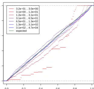
Figure S2: Empirical cumulative density function (ECDF) plots for theχ2_{-probabilities of the residuals from the variance}

fit (orange line in Figure 1), stratified by the mean. The green line is the diagonal, which is the expected curve if the residuals follow theχ2_{distribution withm}

ρ−1 = 1 degree of freedom.

2000) in the C API of R (R Development Core Team, 2009).

E

Diagnostics for the local

re-gression

The choice of the gamma family for the local regression can be motivated as follows: If the size-adjusted counts

kij/sj in the sample variance estimatewiρ calculated

in Equation (7) were normally distributed with true varianceσ_ij2, the quantity (mρ−1)wiρ/σ2ijwould follow

a χ2_{distribution withm}

ρ−1 degrees of freedom, and

this should hold as well for the residuals,

ξiρ= (mρ−1)

wiρ

w(ˆqiρ)

(where we have replaced the true variance σ2_{with its}

fitted value w(ˆqiρ.) . Even though the size-adjusted

counts are not normally distributed, this is still a use-ful approximation for GLM local regression. Among the exponential families commonly used with general-ized linear models, the gamma family, which includes theχ2distributions, is close to the actual distribution of the residuals, and since generalized linear models tend to show robustness against misspecification, we expect a reasonable fit. In order to verify this, we

0.0 0.2 0.4 0.6 0.8 1.0 0.0 0.2 0.4 0.6 0.8 1.0 p value ECDF edgeR DESeq

p value from edgeR

p v

alue from DESeq

10^−10 10^−5 10^0

10^−10 10^−5 10^0

Figure S3: Results from a simulation mimicking the distribution of counts in the neural stem cell data. (a) Uniformity of thep

values calculated for the genes that were not differentially expressed, shown with an ECDF plot. (b) Comparison of thepvalues between theDESeqandedgeRfor the genes that were simulated as differentially expressed.

can check how well the residuals ξiρ follow a χ2

dis-tribution. To this end, we calculate theχ2 _quantiles

of theξiρ and check them for uniformity by plotting

their empirical cumulative density function (ECDF). Figure S2 shows the ECDF curves for the condition

ρ= GNS, stratified by the estimated means ˆqiρ. As

one can see, the residuals follow the distribution rea-sonably well. Only for extremely low counts (below 5), the fitting quality is reduced. At such low counts, the shot noise dominates (see Figure 1b), and inaccu-racies in the estimation of the raw noise are no reason for concern.

It is worth noting that the χ2 _{distribution for}

mGNS−1 = 1 degree of freedom has a heavy right

tail. Hence, the fact that in Figure 1 so many points lie far above the fitted line does not imply a bad fit.

F

Simulations

As a check of the correctness ofDESeq and to further explore its performance in comparison to edgeR, we performed simulations. Here, we show a set of typical results for simulation parameters chosen to resemble the situation in the neural stem cell data set.

We drew true mean valuesqi for 20,000 genes from

an exponential distribution with rate 1/250. Each gene was considered “truly differentially expressed” (tDE) with probability 30%, and for all tDE genes

a log₂ fold change was randomly drawn from a nor-mal distribution with mean 0 and standard deviation 2.5. Finally, four count values were drawn for each gene, two for condition A and two for condition B, from negative binomial distributions, with the given means and variances as below, and multiplied by the size factors, which we chose as 0.5, 1.7, 1.4 and 0.9, similar to those seen in experimental data

For the variances, we catered toedgeR’s assumption and set the raw SCV to a constant, 0.5. Then, we used both our approach andedgeRto test for differential ex-pression. edgeR was given the true size factors, while our approach had to estimate them from the data. In this setting,edgeR (running in common-dispersion mode) correctly estimated the raw SCV with good ac-curacy. Both approaches controlled the type-I error rate correctly: the percentage of type-I errors at 5% nominal significance level was (averaged over 10 simu-lation runs) 3.1% for DESeq and 3.4% for edgeR. (See Figure S3a for a plot with data from one run). At 10% FDR, DESeq discovered 21% of the truly differentially expressed genes, and edgeR found 26%. Finally, both methods stayed below the nominal 10% FDR with an actual FDR of 5.1% (DESeq) and 6.9% (edgeR). Note that edgeR’s apparent slight advantage is to be ex-pected here as the simulation stipulates a constant raw SCV.