(will be inserted by the editor)
A spatio-temporal model for Red Sea surface
temperature anomalies
Christian Rohrbeck1,2 · Emma S. Simpson1 · Ross P. Towe3,4
Received: date / Accepted: date
Abstract This paper details the approach of teamLancasterto the 2019 EVA data challenge, dealing with spatio-temporal modelling of Red Sea surface temperature anomalies. We model the marginal distributions and dependence features separately; for the former, we use a combination of Gaussian and generalised Pareto distributions, while the dependence is captured using a localised Gaussian process approach. We also propose a space-time moving estimate of the cumulative distribution function that takes into account spatial variation and temporal trend in the anomalies, to be used in those regions with limited available data. The team’s predictions are compared to results obtained via an empirical benchmark. Our approach performs well in terms of the threshold-weighted continuous ranked probability score criterion, chosen by the challenge organiser.
Keywords Extreme value analysis · Gaussian processes · Red Sea ·
Spatio-temporal dependence
1 Introduction
Understanding the behaviour of environmental processes, such as precipita-tion, wind speed or temperature, is critical for a number of applications, in-cluding weather forecasting and predicting the effects of climate change (Coo-ley et al., 2007; Towe et al., 2017; Rohrbeck et al., 2018). Interest in these environmental processes can be at a single location or over large spatial ar-eas, as well as over a range of time periods. For example, questions of interest Christian Rohrbeck (corresponding author)
E-mail: cr777@bath.ac.uk
1Department of Mathematics and Statistics, Lancaster University, LA1 4YF, UK. 2Department of Mathematical Sciences, 4 West, University of Bath, BA2 7AY, UK. 3School of Computing and Communications, Lancaster University, LA1 4WA, UK. 4Shell U.K. Limited, London, UK.
may be what percentage of the United Kingdom will observe a mean average temperature of above 15◦C for the month of May, or what is the expected maximum Red Sea surface temperature in 2050.
In some instances, interest lies in the largest values of a spatial process, such as determining the likely spatial extent of a flood event or a heatwave; ex-ample methods and applications can be found in Davison et al. (2012), Winter et al. (2016) and Tawn et al. (2018). Approaches include max-stable processes (Smith, 1990; Schlather, 2002) and Pareto processes (Ferreira and de Haan, 2014); these are applicable when locations experience concomitant extremes, which may not always be the case. More recent literature that addresses this issue includes work based on Laplace random fields (Opitz, 2016), the Gaus-sian scale mixture model of Huser et al. (2017), and the conditional spatial model of Wadsworth and Tawn (2019). Review papers on the topic of spatial extremes include Davison and Huser (2015) and Davison et al. (2019).
There has been work to extend some of these approaches for modelling spatio-temporal dependence. While a range of statistical techniques, such as Gaussian processes, exist for analysing spatio-temporal data (Cressie and Wikle, 2011; Wikle et al., 2019), current spatio-temporal extremes models are limited to problems of moderate dimensions. For example, spatio-temporal max-stable processes are considered by Davis et al. (2013) and Huser and Davison (2014), but these models suffer from being computationally expensive to fit. Alternative approaches include the skew-tmodel of Morris et al. (2017), and a space-time extension of the conditional extremes approach (Simpson and Wadsworth, 2020), neither of which are currently feasible for the very high number of dimensions we will consider here. A key aspect that unites these models and applications is the importance of understanding the spatio-temporal dependence.
Our analysis focuses on gaining a better understanding of Red Sea surface temperatures. The Red Sea supports a rich and diverse ecosystem and these high temperatures may result in coral bleaching. This degradation of the bio-diversity of the Red Sea could have an impact on the local economy, with the north-west coast being a particularly popular tourist destination (Fine et al., 2019). This will also have impact on the fishing industries in the area that support a number of communities situated around the Red Sea. Previous studies such as Allison et al. (2009) and Brander (2010) have investigated the complex impacts of climate change on fisheries. As a result, it is important to understand the changing behaviour of the Red Sea and determine which regions are more susceptible to global warming. Examples of existing extreme value analyses of Red Sea surface temperatures can be found in Hazra and Huser (2020) and Simpson and Wadsworth (2020).
The Red Sea surface temperature data for this challenge are not direct measurements, but are instead daily anomalies available from the period 1985-2015, with the Red Sea being discretised into 16703 grid cells (locations). Data for some of the locations and times have been artificially removed. The aim of the challenge was to issue a probabilistic forecast of the temperature anoma-lies within specific space-time regions; predictive performance of our proposed
model against the benchmark was assessed by using a specific metric, in this case the threshold-weighted continuous ranked probability score (twCRPS) of Gneiting and Ranjan (2011). For more details on the data set and the chal-lenge, see Huser (2020).
In order to model the sea surface temperature anomalies, we adopt a two-step approach which accounts for spatio-temporal variations in the marginal behaviour and dependence structure. The marginal behaviour at a spatial lo-cation is modelled via an extreme mixture model, which allows us to capture differences in the body and tails of the data. We find interesting spatial varia-tions in the model parameters, and these can be linked to geographical features of the Red Sea. Conditional on the fitted marginal models, spatio-temporal dependence is then modelled by using a localised Gaussian process. While Gaussian processes imply a restrictive spatio-temporal dependence structure on the extremes, existing spatial extreme methods are too computationally expensive for large data sets. For those locations with insufficient data to fit a Gaussian process, the predictive distribution is estimated through pooling the observed data over a spatio-temporal window.
The paper is structured as follows: Section 2 details the data analysis and the methods used to model both the marginal and dependence behaviour of the sea surface temperature anomalies; Section 3 assesses performance with respect to the provided benchmark estimate and the twCRPS; Section 4 concludes with a discussion of the ways in which the analysis could be improved.
2 Methods and Data Analysis
2.1 Exploratory data analysis
2.1.1 Challenge description and benchmark prediction
Let Y(s, t) be the sea surface temperature recorded at grid cell s∈ S ⊂ R2
and timet∈ T ={1, . . . , T}, where|S|= 16703 andT = 11315. Our analysis focuses on the anomalies
A(s, t) =Y(s, t)−µˆ(s, t),
where ˆµ(s, t), (s, t) ∈ X = S × T, is an estimated mean effect. Parts of the anomaly data {A(s, t) : (s, t)∈ X } were masked artificially by the EVA 2019 data competition organiser; see Huser (2020) for more details. We de-note the subset ofX for which anomalies are available byXT and we refer to
{A(s, t) : (s, t)∈ XT}as the training data set.
High temperature events are likely to affect large scale areas for sus-tained periods of time. Therefore interest lies in the distribution of the spatio-temporal minimum rather than the minimum in a particular point in time and space. For each particular space-time point, a local neighbourhoodN(s, t)⊂ X
is constructed. Herein, we consider
whereB(s, r) is a ball centred at locationswith radiusr= 50 km, and we are interested in the smallest anomaly within the local neighbourhood,
X(s, t) = min
(s0,t0)∈N(s,t)A(s
0, t0). (1)
The aim is to predictX(s, t) for certain space-time points within a validation
set XV, (s, t) ∈ XV ⊂ X \ XT, by providing a corresponding distribution
functionFs,t(·); these validation points all lie in the period 2007-2015.
Huser (2020) derives an estimate, termed the benchmark prediction, for the distribution functionFs,t(·), (s, t)∈ XV, in three steps. Firstly, the setNC of
neighbourhoods with no missing values is identified, i.e.NC={(s, t) :N(s, t)⊂ XT}.
Next, the spatio-temporal minima as defined in (1) are determined for the neighbourhoods in NC. Finally, the benchmark prediction for Fs,t(·) is
de-fined as the empirical cumulative distribution function ˆFben of the values
{X(s, t) : (s, t)∈ NC}.
2.1.2 Exploring spatial and temporal features
The benchmark prediction, ˆFben, assumes that the data are stationary in
space and time. Evidence suggests that this assumption may not be valid. As an illustrative example, we focus on the temporal component (the same idea holds for the spatial component) and separate the data into two time horizons H and H∗, where H = {1, . . . , T∗} and H∗ = {T∗+ 1, . . . ,11315}
withT∗∈(1,11315).
We can test whether there is a difference between the empirical cumulative distribution functions evaluated in these two time horizons, denoted ˆFben
H and
ˆ
FHben∗. We adopt the two-sample Kolmogorov-Smirnov test to detect whether there is any change in the distribution function. The Kolmogorov-Smirnov test statistic is DH,H∗ = sup x∈R ˆ FHben(x)−FˆHben∗(x) ,
where sup is the supremum function, andDH,H∗is tested against a 5% signif-icance level.
We choose T∗ = 8030, which is equivalent to separating the data into
two time periods: 1985-2006 and 2007-2015. The estimated test statistic is
DH,H∗ = 0.125, corresponding to a p-value of 0.004. Thus, we reject the hy-pothesis that the cumulative distribution function remains stationary over the time period.
We are also interested in how the spatial dependence changes as a function of distance. The variogram can be used to determine the spatial dependence of the spatial processY and is given by
2δ(w, w0) = Var[Y(w)−Y(w0)],
for two particular sites (w, w0), whereδis the semi-variogram function (Math-eron, 1963). If the process Y is stationary, then δ(w, w0) = δ(w−w0). The
variogram explains the spatial dependence of average values of the process, however our interest also lies in how the spatial dependence changes for the largest values of the process. The F-madogram is an equivalent function to the variogram that instead describes the spatial dependence of the extremes (Cooley et al., 2006). The F-madogram is given by
ν(w, w0) = 1
2E[F(Y(w))−F(Y(w
0))],
whereF is the distribution function of the spatial process.
These two functions help us to determine the dependence structure of the anomaly data and plots are provided in the Appendix. Across subsets ofS, the empirical variograms indicate a variation in the spatial dependence structure, while the F-madograms exhibit a similar spatial dependence for the highest anomalies. We further examine a potential trend in the dependence by esti-mating variograms and F-madograms for the horizonsH ={1, . . . ,5000}and
H∗={5001, . . . , T = 11315}. We find little, or no, change in the dependence
of the highest anomalies, while the overall spatial dependence increases slightly for some parts of Red Sea.
2.1.3 Space-time moving cumulative distribution function
The main method we propose in Section 2.2 relies on there being sufficient data in a space-time neighbourhood of each validation point (s, t)∈ XV. For those
validation points with insufficient data, we could resort to using the benchmark prediction ˆFben, given in Section 2.1.1. However, since there is some evidence
of non-stationarity in X(s, t), we propose to alter this slightly by deriving cumulative distribution functions across local space-time moving cylinders. Instead of pooling all of those locations that have complete observations, we use a neighbourhoodN∗(s, t) with
N∗(s, t) ={B(s, r)× {t−365, . . . , t, . . . , t+ 365}} ∩ X,
whereB(s, r) is a ball centred at locationswith radius r= 75 km. The esti-mate ˆFs,t∗ (·) forFs,t(·), (s, t)∈ XV, is then derived as the empirical cumulative
distribution function of observations in{X(s0, t0) : (s0, t0)∈ NC∩ N∗(s, t)}.
For some of the validation points (s, t)∈ XV, the neighbourhoodN(s, t)
contains space-time points for which the anomalies are available, i.e.N(s, t)∩ XT 6=∅. Then, X(s, t) cannot be larger than any of the observed anomalies
{A(s0, t0) : (s0, t0)∈ N(s, t)∩ XT}. Therefore, the minimum observed anomaly
within the neighbourhoodN(s, t) provides an upper bound forX(s, t). We take
this property into account by setting ˆFs,t∗ (x) = 1 forx≥min{A(s0, t0) : (s0, t0)∈ N(s, t)∩ XT}.
2.2 Spatio-temporal model 2.2.1 Introduction
The empirical distribution derived in Section 2.1.3 captures large-scale spatio-temporal trends inX(s, t) (s∈ S;t∈ T), but does not account for short-term variations in the anomalies which the challenge asks us to predict. This section introduces our model for these short-term variations. Instead of{X(s, t) : (s, t)∈ X }, we first model the process{A(s, t) : (s, t)∈ X }, and then derive our estimates for{Fs,t(·) : (s, t)∈ XV}.
Section 2.1.2 shows that the data exhibit spatio-temporal dependence. This motivates pooling data across nearby space-time points in the training data set XT to model the anomaly A(s0, t0), where (s0, t0) ∈ X \ XT refers to a
space-time point for which the recorded anomaly is not available. We may consider modelling{A(s, t) : (s, t)∈ X }via a Gaussian process. However, such an approach would have to account for, amongst others, the spatial variation in both the dependence structure and the marginal distributions of the anomalies. We address these aspects in two modelling steps. In the first step, we fit a marginal model to the observed values ofA(s,1), . . . , A(s, T) separately for each grid cell s ∈ S in Section 2.2.2, yielding an estimated distribution function Gs(·). We then consider the process of transformed random
vari-ables{U(s, t) =Gs[A(s, t)] : (s, t)∈ X }, which provides approximate uniform
marginal distributions for each grid cell. In the second step, in Section 2.2.3, we model the non-stationary process{U(s, t) : (s, t)∈ X }and derive estimates for{Fs,t(·) : (s, t)∈ XV}.
2.2.2 Marginal modelling
Since the anomalies represent deviations from an estimated mean, we first test whether A(s,1), . . . , A(s, T) (s ∈ S) are normally distributed; for nota-tional brevity, we drop the location indexsin the rest of this subsection. The Lilliefors test (Lilliefors, 1967) rejects the null hypothesis of A(1), . . . , A(T) being normally distributed at the 1% significance level for 13,200 of the 16,703 locations. A closer examination of the model fit indicates that the normal distribution is poor at capturing the lower and upper tail behaviour of the anomalies, while providing a very good fit for the bulk of the distribution.
Extreme value theory provides us with an asymptotically justified mod-elling framework for the highest (lowest) values of a continuous random vari-able Z. We adopt a peaks-over threshold approach and consider Z | Z > u
(u∈R). For some suitably high threshold u, exceedances byZ ofuare mod-elled using the generalised Pareto distribution GPD(ψ, ξ) with
P(Z ≤z+u|Z > u) = 1− 1 +ξz ψ −1/ξ + := H(z;ψ, ξ) (z >0),
where {z}+ = max{0, z}, and (ψ, ξ) ∈ R+×R are the scale and shape
arises as the only possible non-degenerate limit for scaled excesses of Z as u
tends to the upper end point of the distribution. The lower tail of Z is mod-elled in the same way by first picking a sufficiently small threshold`and then fitting a generalised Pareto distribution using that P(Z < `−z|Z < `) =
P(−Z > z−`| −Z >−`).
To improve upon the marginal fit of the normal model, we define an ex-treme mixture model (Frigessi et al., 2002; Behrens et al., 2004; MacDonald et al., 2011) which provides more flexibility regarding the tail behaviour of the distribution functionG(·). Given thresholds`andu(` < u), observations are modelled as being normally distributed within the interval [`, u], and gen-eralised Pareto distributed otherwise, with separate parameters (ψ`, ξ`) and
(ψu, ξu) for the lower and upper tail, respectively. The distribution function is
thus G(a) = Φ `−µ σ [1−H(`−a;ψ`, ξ`)] ifa < `, Φ a−µ σ if`≤a≤u, Φ u−µ σ + 1−Φ u−µ σ H(a−u;ψu, ξu) ifa > u, (2) whereΦ(·) denotes the standard normal cumulative distribution function.
Prior to estimating the spatially varying model parameters (µ, σ, ψ`, ξ`, ψu, ξu)
in (2), we consider threshold stability plots (Coles, 2001) for a subset of 50 grid cells. As a result, we choose the empirical 6% and 94% quantiles of the observed anomaliesA(1), . . . , A(T) as thresholds `andu, separately for each grid cell. Parameter estimates are derived using likelihood inference; note that for fixed`andu, (µ, σ) can be estimated independently of (ψ`, ξ`) and (ψu, ξu).
Figure 1 demonstrates the estimated model parameters over space, indi-cating a north-south trend in the marginal behaviour of the anomalies. In-terestingly, the strong north-south trend for σ correlates with topographical features of the Red Sea; the water in the northern Red Sea is generally deeper than in the southern Red Sea. When studying the tail behaviour, most esti-mates for the shape parametersξ` and ξu are negative, corresponding to the
distribution ofA1, . . . , AT being short-tailed with finite lower and upper end
points; this agrees with previous studies on extreme low and high temperatures (Thibaud et al., 2016; Winter et al., 2016). We also calculate the site-wise 80% and 90% quantiles of the estimated GPD distributions. Similarly toσ, we find a north-south decrease in these quantiles, with the trend being stronger in the upper tail. Consequently, anomalies in the northern Red Sea appear to be more variable than in the southern Red Sea. To assess the fit of the extreme mixture model (2), we examine the quantile-quantile plots for two locations in Figure 2. The plots show a very good overall fit and illustrate that the lower and upper tail behaviour are well captured.
15 20 25 30 32 36 40 44 Longitude Latitude −0.08 −0.04 0.00 µ 15 20 25 30 32 36 40 44 Longitude Latitude 0.5 0.6 0.7 0.8 σ 15 20 25 30 32 36 40 44 Longitude Latitude 0.2 0.3 0.4 0.5 ψl 15 20 25 30 32 36 40 44 Longitude Latitude −0.4 −0.2 0.0 ξl 15 20 25 30 32 36 40 44 Longitude Latitude 0.2 0.3 0.4 0.5 ψu 15 20 25 30 32 36 40 44 Longitude Latitude −0.4 −0.3 −0.2 −0.1 0.0 0.1 ξu
Fig. 1 Parameter estimates (ˆµ,σˆ) (top), ( ˆψ`,ξˆ`) (middle) and ( ˆψu,ξˆu) (bottom) for the
−2 −1 0 1 2 −2 −1 0 1 2 3 Estimated quantiles Empir ical quantiles −2 −1 0 1 2 −2 −1 0 1 2 Estimated quantiles Empir ical quantiles
Fig. 2 Quantile-quantile plots for the grid cells with spatial index 3500 (left) and 9000 (right). The solid line represents the fit for a normal distribution, while the dashed line corresponds to the extreme mixture model fit. The dotted vertical lines are the thresholds
`anduused in the extreme mixture model.
2.2.3 Dependence modelling
We now require a model to capture the spatio-temporal dependence between the anomalies. For spatial extremes, a variety of such models exist, but the spatio-temporal case is less well-studied in the literature. The most well-known models for spatio-temporal extremes are max-stable processes (Davis et al., 2013; Huser and Davison, 2014), however, currently available inferential meth-ods are computationally expensive, and cannot handle the large number of space-time locations we wish to study. We instead propose the use of Gaus-sian processes to model the spatio-temporal dependence. As well as bringing computational efficiency to our approach, they facilitate the simulation of ob-servations for locations with missing data, allowing us to estimate the distri-bution of the processX(s, t) for space-time locations in the validation setXV
via a conditional approach.
Consider a Gaussian process {Z(w) : w ∈ Rm} with mean function µ : Rm → R and covariance function ρ(w1, w2), for w1, w2 ∈ Rm. In our
appli-cation, we are interested in the Gaussian process at a finite set of space-time locations (s, t)1, . . . ,(s, t)n ∈ S × T. The process at these locations follows
a multivariate Gaussian distribution with mean vector µ ∈ Rn and
covari-ance matrixΣ ∈Rn×n, obtained via the covariance function ρ. Suppose we
want to generate observations for the first n1 space-time locations,
condi-tioning on observations at a further n2 locations. The mean vector µ and
covariance matrix Σ can be partitioned to represent these two sets of loca-tions, i.e., µ= (µ1,µ2) for µ1 ∈Rn1 andµ2∈Rn2, andΣ =
Σ11Σ12 Σ21Σ22 for Σ11∈Rn1×n1,Σ 12∈Rn1×n2,Σ 21∈Rn2×n1 andΣ 22∈Rn2×n2. Conditioning
on observationsz ∈Rn2 at space-time locations (s, t)
generate observations for locations (s, t)1, . . . ,(s, t)n1 by sampling from a
mul-tivariate Gaussian distribution with mean vector µ∗ and covariance matrix
Σ∗given by
µ∗=µ1+Σ12Σ22−1(z−µ2); Σ∗=Σ11−Σ12Σ−221Σ21.
In order to focus on modelling the dependence of our temperature anoma-lies, we consider fitted quantiles at each spatial location, defined by ˆu(s, t) =
ˆ
Gs{A(s, t)} ∈[0,1], where ˆGs denotes the fitted extreme mixture model (2)
at locations. To obtain values on a scale conducive to Gaussian process mod-elling, we apply a probit transformation to these empirical quantiles, obtaining
z(s, t) =Φ−1[ˆu(s, t)]∈(−∞,∞),
for each (s, t)∈ XT;Φ−1denotes the inverse cumulative distribution function
of the standard normal distribution. Then, the marginal observations for grid cells∈ S,z(s,1), . . . , z(s, T), are Normal(0,1) distributed. However, the size of the data makes the estimation of a single Gaussian process acrossS × T
infeasible inR.
Instead, we fit a local Gaussian process separately for each (s, t) ∈ XV,
using non-missing values ofz(s, t) at locations within a space-time cylinder
N0(s, t) ={B(s, r0)× {t−3, t−2, t−1, t, t+ 1, t+ 2, t+ 3}} ∩ X.
Here, B(s, r0) denotes a ball centred at s with some radius r0 > r, i.e.,
N0(s, t)⊃ N(s, t). We take an exponential separable covariance function, ρ{(s, t)1,(s, t)2}= exp −|s1,lon−s2,lon| φlon −|s1,lat−s2,lat| φlat −|t1−t2| φtime ,
with (s, t)1,(s, t)2 ∈ S × T and | · | denoting the absolute difference. In our
analysis, we generally find thatφtimeis larger thanφlonandφlat, corresponding
to consecutive daily anomalies for the same grid cell being more dependent than the anomalies for two grid cells on the same day which are 1◦in longitude (latitude) apart.
The radius r0 is initially set to 60km, and increased in 10km increments until the cylinderN0(s, t) contains at least 100 points, up to a maximum radius
of 150km. This approach ensures sufficient data to estimate the parameters of the Gaussian process, while still accounting for spatial trends in the data. We fit these Gaussian process models using the packageDiceOptiminR(Picheny et al., 2016), and generate 500 samples for each missing observation within the original space-time cylinderN(s, t), using the conditional simulation approach detailed above. For those validation locations with less than 100 available data points inN0(s, t) at radiusr0= 150km, we use the distribution function
obtained via the space-time moving cylinders discussed in Section 2.1.3. Having generated these observations for the space-time locations with miss-ing data, we transform back to the interval [0,1] using the cumulative normal distribution function, and transform to the original scale using the marginal
fits discussed in Section 2.2. Taking the minimum observation in N(s, t) for each sample results in 500 simulations of X(s, t) for each (s, t)∈ XV. We
fi-nally use these observations to empirically estimate the required distribution function.
3 Results
3.1 Comparison to the benchmark
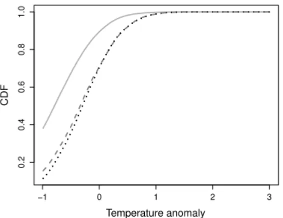
We first compare our method to the empirical approach used to calculate the benchmark. In Figure 3, we present the benchmark CDF, as well as a recalculated benchmark using data only from the validation period (2007 to 2015). We also present results for our proposed method, by averaging our predicted distributions across all space-time locations inXV, i.e., we take the
average CDF for each anomaly value where the distribution functions are evaluated. −1 0 1 2 3 0.2 0.4 0.6 0.8 1.0 Temperature anomaly CDF
Fig. 3 A comparison of the original benchmark (solid line); a version of the benchmark for the validation period only (dashed line); and the average of our estimated CDFs for all locations inXV (dotted line).
Here, we observe a clear difference in the results obtained via the bench-mark approach computed for the training data with complete neighbourhoods and observations within the validation period, particularly for anomalies in the range [−1,1]. This disparity highlights the existence of a temporal trend in the anomaly data (see Section 2), and supports our use of a localised approach. On average, our method closely agrees with the empirical results within the valida-tion period, demonstrating that, overall, we are able to capture this temporal behaviour.
3.2 Evaluation of the score
We further examine the performance of our approach using the threshold-weighted continuous ranked probability score (twCRPS) from the data chal-lenge. Let ˆFs,tbe the predicted distribution function for the minimum anomaly
X(s, t) overN(s, t), and denote the true value byx(s, t). The twCRPS is then approximated by 1 100 400 X k=1 h ˆ Fs,t xk −1 x(s, t)≤xk i 2 Φ xk−1.5 0.4
wherexk=−1+k/100 (k= 1, . . . ,400). We select a test data setX∗⊂ X
con-taining 4,200 space-time locations, such that no data are missing overN(s, t) for (s, t)∈ X∗. Data are then randomly removed fromN(s, t) for (s, t)∈ X∗;
the amount of missing data is sampled from the empirical distribution function of missing values withinN(s0, t0) for (s0, t0)∈ XV. We generate five such data
sets for each (s, t)∈ X∗, with the aim to recover the true valuex(s, t) using
our approach in Section 2.
The approximated score across the test points in X∗ is 0.17×10⁻⁴. The
discrepancy between the scores for the setX∗and the validation setX
V used
by Huser (2020) is subsequently explained. Firstly, our generated test data is only similar to the validation data with respect to the number of missing data points within the 50km radius. However, the test data exhibit less missing observations within the 150km radius, and our Gaussian process approach can thus be applied more often. In particular, the space-time moving cumulative distribution function had to be derived only once for the points inX∗, while
we had to use it for 15% of the space-time points inXV. The second reason
for the discrepancy in the scores is thatX∗ covers the years 1985-2015 while
the challenge considers the period 2007-2015. Given the positive trend in the anomalies, and the fact that the twCRPS gives more weight to predicting high values ofX(s, t), a higher average score is to be expected for space-time points in the later years.
4 Discussion
We thank Rapha¨el Huser for organising this data challenge. Our approach utilised tools from spatial statistics and extreme value analysis, and could be extended. For instance, other teams showed that machine learning techniques can be applied successfully to recover the missing values in the data. It would be interesting to explore whether a combination of these approaches could yield better results. Specifically, our localised Gaussian process estimates may potentially be replaced by their approaches. The implementation of a cross-validation scheme would help to distinguish the advantages and disadvantages of both approaches.
One drawback of using Gaussian processes for extreme value modelling, is their ability to capture only asymptotic independence, i.e., situations where
the largest values occur separately across different variables. The development of computationally efficient models that are able to capture both asymptotic dependence and asymptotic independence is a topic that still requires atten-tion, and it is likely that our approach would be improved by the added flex-ibility such models would bring. Conditional models for extremes (Heffernan and Tawn, 2004; Wadsworth and Tawn, 2019), which are able to capture these different tail dependence classes as well as allowing for straightforward sim-ulation of missing data, have recently been extended to the spatio-temporal setting by Simpson and Wadsworth (2020), and provide one possible avenue for the improvement of our approach.
Another extension may be to address the temporal non-stationarity in the marginal behaviour of the anomalies. We again used the Lilliefors test to decide whether the anomalies may be modelled via a normal distribution. The data were split into blocks of length 500 days, and the null hypothesis was rejected for 30%-80% of locations on the 5% significance level across blocks. Next, we considered the two time seriesA(1), . . . , A(5000) and A(5001), . . . , A(T) and fit separate extreme mixture models. The thresholds` and uwere set to the empirical 6% and 94% quantiles of the respective time series. The mean pa-rameter µ was higher for the second time period for all locations, and the highest difference was found for the central Red Sea. Further, σ was higher in the first period for most locations, except the most northern and southern locations. Finally, the 80% quantiles of the GPD for the lower tail were similar across the two periods, while the 80% quantiles of the GPD(ψu, ξu) were on
average slightly shorter in the second period. In addition to a temporal trend, we considered seasonality in the parameters of the extreme mixture model; the estimates were very similar for all seasons. In summary, we found a positive trend in the mean of the anomalies and a negative trend in their variation. Fur-thermore, the results indicated that the temporal trend in marginal behaviour varies across locations. To capture these features, one may define a spatio-temporal model for each of the parameters; however, we did not investigate this aspect further due to time constraints.
Appendix: Empirical analysis of the spatial and extremal spatial dependence
We produce variograms and F-madograms for the four sub-regions in Figure 4. The left column in Figure 5 shows that spatial dependence varies across sub-regions. Furthermore, there appears to be a temporal variation in the spatial dependence for two of the sub-regions. The right column of Figure 4 indicates that the extremal spatial dependence exhibits less spatial variation than the overall spatial dependence. Furthermore, the plots demonstrate slight changes in the extremal spatial dependence, but not as strong as for the overall spatial dependence.
32 34 36 38 40 42 44 15 20 25 30 Longitude Latitude
Fig. 4 Subregions used to explore spatial and extremal dependence.
Acknowledgements We would like to thank the referees and Associate Editor for their
helpful comments. Christian Rohrbeck is beneficiary of an AXA Research Fund postdoctoral grant. Emma Simpson’s work is supported by the King Abdullah University of Science and Technology (KAUST) Office of Sponsored Research (OSR) under Award No. OSR-CRG2017-3434. Ross Towe is supported by Engineering and Physical Sciences Research Council (Grant Number: EP/P002285/1) ‘The Role of Digital Technology in Understanding, Mitigating and Adapting to Environmental Change’.
Conflict of interest
The authors declare that they have no conflict of interest.
References
Allison, E. H., Perry, A. L., Badjeck, M.-C., Adger, W. N., Brown, K., Conway, D., Halls, A. S., Pilling, G. M., Reynolds, J. D., Andrew, N. L., and Dulvy, N. K. (2009). Vulnerability of national economies to the impacts of climate change on fisheries. Fish and Fisheries, 10(2):173–196.
Behrens, C. N., Lopes, H. F., and Gamerman, D. (2004). Bayesian analysis of extreme events with threshold estimation. Statistical Modelling, 4(3):227– 244.
Brander, K. (2010). Impacts of climate change on fisheries. Journal of Marine Systems, 79(3-4):389–402.
Coles, S. G. (2001).An Introduction to Statistical Modeling of Extreme Values. Springer Series in Statistics. Springer-Verlag London.
Cooley, D., Naveau, P., and Poncet, P. (2006). Variograms for spatial max-stable random fields. In Dependence in Probability and Statistics, pages 373–390. Springer.
Cooley, D., Nychka, D., and Naveau, P. (2007). Bayesian spatial modeling of extreme precipitation return levels. Journal of the American Statistical Association, 102(479):824–840.
0.2 0.4 0.6 0.8 1.0 1.2 0.00 0.04 0.08 0.12 Distance V ar iogr am 0.2 0.4 0.6 0.8 1.0 1.2 0.00 0.02 0.04 0.06 0.08 Distance F−Madogr am 0.2 0.4 0.6 0.8 1.0 0.00 0.04 0.08 0.12 Distance V ar iogr am 0.2 0.4 0.6 0.8 1.0 0.00 0.02 0.04 0.06 0.08 Distance F−Madogr am 0.2 0.4 0.6 0.8 1.0 0.00 0.04 0.08 0.12 Distance V ar iogr am 0.2 0.4 0.6 0.8 1.0 0.00 0.02 0.04 0.06 0.08 Distance F−Madogr am 0.2 0.4 0.6 0.8 1.0 0.00 0.04 0.08 0.12 Distance V ar iogr am 0.2 0.4 0.6 0.8 1.0 0.00 0.02 0.04 0.06 0.08 Distance F−Madogr am
Fig. 5 Variograms (left) and F-Madograms (right) for the four subregions in Figure 4. The black curve corresponds to the time horizont= 1, . . . ,5000, and the grey curve corresponds to the periodt= 5001, . . . ,11315. The dashed lines are the central 80% confidence intervals.
Cressie, N. and Wikle, C. K. (2011).Statistics for Spatio-Temporal Data. John Wiley & Sons.
Davis, R. A., Kl¨uppelberg, C., and Steinkohl, C. (2013). Statistical inference for max-stable processes in space and time. Journal of the Royal Statistical Society. Series B (Statistical Methodology), 75(5):791–819.
Davison, A. C. and Huser, R. (2015). Statistics of extremes. Annual Review of Statistics and its Application, 2:203–235.
Davison, A. C., Huser, R., and Thibaud, E. (2019). Spatial extremes. In A. E. Gelfand, M. Fuentes, J. A. H. and Smith, R. L., editors,Handbook of Environmental and Ecological Statistics. CRC Press.
Davison, A. C., Padoan, S. A., and Ribatet, M. (2012). Statistical modeling of spatial extremes. Statistical Science, 27(2):161–186.
Ferreira, A. and de Haan, L. (2014). The generalized Pareto process; with a view towards application and simulation. Bernoulli, 20(4):1717–1737. Fine, M., Cinar, M., Voolstra, C. R., Safa, A., Rinkevich, B., Laffoley, D.,
Hilmi, N., and Allemand, D. (2019). Coral reefs of the Red Sea - challenges and potential solutions. Regional Studies in Marine Science, 25:100498. Frigessi, A., Haug, O., and Rue, H. (2002). A dynamic mixture model for
un-supervised tail estimation without threshold selection. Extremes, 5(3):219– 235.
Gneiting, T. and Ranjan, R. (2011). Comparing density forecasts using threshold- and quantile-weighted scoring rules. Journal of Business & Eco-nomic Statistics, 29(3):411–422.
Hazra, A. and Huser, R. (2020). Estimating high-resolution Red Sea sur-face temperature hotspots, using a low-rank semiparametric spatial model. arXiv:1912.05657.
Heffernan, J. E. and Tawn, J. A. (2004). A conditional approach for multi-variate extreme values (with discussion). Journal of the Royal Statistical Society. Series B (Statistical Methodology), 66(3):497–546.
Huser, R. (2020). Editorial: EVA 2019 data competition on spatio-temporal prediction of Red Sea surface temperature extremes.Extremes (To Appear). Huser, R. and Davison, A. C. (2014). Space-time modelling of extreme events. Journal of the Royal Statistical Society. Series B (Statistical Methodology), 76(2):439–461.
Huser, R., Opitz, T., and Thibaud, E. (2017). Bridging asymptotic indepen-dence and depenindepen-dence in spatial extremes using Gaussian scale mixtures. Spatial Statistics, 21(A):166–186.
Lilliefors, H. W. (1967). On the Kolmogorov-Smirnov test for normality with mean and variance unknown. Journal of the American Statistical Associa-tion, 62(318):399–402.
MacDonald, A., Scarrott, C. J., Lee, D., Darlow, B., Reale, M., and Russell, G. (2011). A flexible extreme value mixture model. Computational Statistics & Data Analysis, 55(6):2137–2157.
Matheron, G. (1963). Principles of geostatistics. Economic Geology, 58(8):1246–1266.
Morris, S. A., Reich, B. J., Thibaud, E., and Cooley, D. (2017). A space-time skew-tmodel for threshold exceedances. Biometrics, 73(3):749–758. Opitz, T. (2016). Modeling asymptotically independent spatial extremes based
on Laplace random fields. Spatial Statistics, 16:1–18.
Picheny, V., Ginsbourger, D., Roustant, O., with contributions by M. Binois, Chevalier, C., Marmin, S., and Wagner, T. (2016). DiceOptim: Kriging-Based Optimization for Computer Experiments. R package version 2.0.
Pickands, J. (1975). Statistical inference using extreme order statistics. The Annals of Statistics, 3(1):119–131.
Rohrbeck, C., Eastoe, E. F., Frigessi, A., and Tawn, J. A. (2018). Extreme value modelling of water-related insurance claims. The Annals of Applied Statistics, 12(1):246–282.
Schlather, M. (2002). Models for stationary max-stable random fields. Ex-tremes, 5:33–44.
Simpson, E. S. and Wadsworth, J. L. (2020). Conditional modelling of spatio-temporal extremes for Red Sea surface temperatures. arXiv:2002.04362. Smith, R. L. (1990). Max-stable processes and spatial extremes. Unpublished. Tawn, J. A., Shooter, R., Towe, R. P., and Lamb, R. (2018). Modelling spatial extreme events with environmental applications.Spatial Statistics, 28:39–58. Thibaud, E., Aalto, J., Cooley, D. S., Davison, A. C., and Heikkinen, J. (2016). Bayesian inference for the Brown-Resnick process, with an application to extreme low temperatures. The Annals of Applied Statistics, 10(4):2303– 2324.
Towe, R. P., Eastoe, E. F., Tawn, J. A., and Jonathan, P. (2017). Statistical downscaling for future extreme wave heights in the North Sea. The Annals of Applied Statistics, 11(4):2375–2403.
Wadsworth, J. L. and Tawn, J. A. (2019). Higher-dimensional spatial extremes via single-site conditioning. arXiv:1912.06560.
Wikle, C. K., Zammit-Mangion, A., and Cressie, N. (2019). Spatio-Temporal Statistics with R. Chapman & Hall/CRC, Boca Ration, Fl.
Winter, H. C., Tawn, J. A., and Brown, S. J. (2016). Modelling the effect of the El Ni˜no-Southern Oscillation on extreme spatial temperature events over Australia. The Annals of Applied Statistics, 10(4):2075–2101.