Published by: SAGE
URL: https://doi.org/10.1177/0962280217715663
<https://doi.org/10.1177/0962280217715663>
This version was downloaded from Northumbria Research Link: http://nrl.northumbria.ac.uk/30872/
Northumbria University has developed Northumbria Research Link (NRL) to enable users to access the University’s research output. Copyright © and moral rights for items on NRL are
retained by the individual author(s) and/or other copyright owners. Single copies of full items can be reproduced, displayed or performed, and given to third parties in any format or medium for personal research or study, educational, or not-for-profit purposes without prior permission or charge, provided the authors, title and full bibliographic details are given, as well as a hyperlink and/or URL to the original metadata page. The content must not be changed in any way. Full items must not be sold commercially in any format or medium without formal permission of the copyright holder. The full policy is available online: http://nrl.northumbria.ac.uk/policies.html
This document may differ from the final, published version of the research and has been made available online in accordance with publisher policies. To read and/or cite from the published version of the research, please visit the publisher’s website (a subscription may be required.)
A robust imputation method for missing responses and
covariates in sample selection models
Emmanuel O. Ogundimu
Department of Mathematics, Northumbria University, UK
Gary S. Collins
Centre for Statistics in Medicine, University of Oxford, UK
Abstract
Sample selection arises when the outcome of interest is partially observed in a study. Al-though sophisticated statistical methods in the parametric and non-parametric framework have been proposed to solve this problem, it is yet unclear how to deal with selectively missing covariate data using simple multiple imputation techniques, especially in the ab-sence of exclusion restrictions and deviation from normality. Motivated by the 2003-2004 NHANES data, where previous authors have studied the effect of socio-economic status on blood pressure with missing data on income variable, we proposed the use of a robust imputation technique based on the selection-t sample selection model. The imputation method, which is developed within the frequentist framework, is compared with compet-ing alternatives in a simulation study. The results indicate that the robust alternative is not susceptible to the absence of exclusion restriction- a property inherited from the par-ent selection-t model- and performs better than models based on the normal assumption even when the data is generated from the normal distribution. Applications to missing outcome and covariate data further corroborate the robustness properties of the pro-posed method. We implemented the propro-posed approach within the MICE environment in R Statistical Software.
Key Words: Student-t distribution; Heckman model; Missing data; Multiple imputation; Robust method; MICE package.
3 4 5 6 7 8 9 10 11 12 13 14 15 16 17 18 19 20 21 22 23 24 25 26 27 28 29 30 31 32 33 34 35 36 37 38 39 40 41 42 43 44 45 46 47 48 49 50 51 52 53 54 55 56 57 58 59 60
1
Introduction
Missing data are ubiquitous throughout the social, behavioral and medical sciences. The incompleteness of a data set may lead to results that are different from those that would have been obtained had the data set been completely observed.1 distinguished four different
approaches to the analysis of missing data: analysis of only those subjects who complete the study; analysis of available data; use of a single or multiple imputation techniques to replace the missing observations with plausible values, then analyse the complete data set; and joint modelling of observed data and the missingness process. The choice of the method of analysis depends on the missing data mechanism as characterized by2. Data are missing completely at random (MCAR) when the probability of missing data on a variable is not related to other measured variables and is unrelated to the variable itself. In this case, a complete case analysis could be used. A less restrictive assumption than the MCAR is the missing at random (MAR) missing data assumption. This occurs when the probability of missing data for a variable is related to other measured variables in the model but not on the values of the variable itself. This assumption and the distinctiveness of the parameters in the observed data and missingness process allows the missingness process to be ignorable. Likelihood inference can be used under ignorability. Data are missing not at random (MNAR) when the probability of missing data on a variable is related to the values of the variable, even after adjusting for other variables. Indeed, the validity of inferences made under different statistical methods depends on the assumption made about the missingness process.
In settings where covariates or covariates and outcomes are subject to selective missing, the use of joint modelling of the observed and the non-response process may not be straightforward. Multiple imputation (MI) is commonly used in such settings, where missing values arefilled-in (singly or multiply) to produce complete data. It has been suggested that the outcome variable be included in the imputation of missing covariates in order to preserve the relationships among variables3. This may be challenging for non-monotone missing data patterns. Incidentally, the use of FCS (fully conditional specification) algorithm can simplify the imputation process. This algorithm has been implemented in MICE (Multivariate imputation by chained equations) package in R and STATA. Details of Multiple imputation using MICE can be found in4.
A common misunderstanding about MI is that it is restricted to MAR. While it is certainly true that imputation techniques commonly assume MAR, the theory of MI is completely general and also applies to MNAR missingness5. For example, a pattern-mixture approach to sensitivity analysis, where missing values are imputed under a plausible MNAR scenario, has been proposed6. A tipping point approach or the so-called delta method adds a constant
δ to the imputation to creates a difference in the means of respondents and nonrespondents that is equal to δ (7 p88-89). This requires sensitivity analyses to obtain an appropriate
2 3 4 5 6 7 8 9 10 11 12 13 14 15 16 17 18 19 20 21 22 23 24 25 26 27 28 29 30 31 32 33 34 35 36 37 38 39 40 41 42 43 44 45 46 47 48 49 50 51 52 53 54 55 56 57 58 59 60
mean difference which may not be tenable for observational studies with MNAR missingness, especially the Heckman-type sample selection problem.
Sample selection arises when the outcome of interest can only be observed in a subset of the population under study. The data are MNAR because the observed data do not represent a random sample from the population, even after controlling for covariates. A model for selected sample was introduced by8 and several extensions in the parametric framework9–12,
semi-parametric framework13 and non-parametric framework14 have been proposed. Earlier review
of sample selection models can be found in15. A unified approach to parametric multilevel
sample selection model was proposed in16.
The use of a sample selection modelling framework as an imputation model for MI has been suggested in the literature12,17. This approach was implemented for missing covariates data
by18 and compared against competing methods. The author implemented the method using
the moment based two-step method because of the perceived computational complexities of the corresponding full information maximum likelihood method (FIML). However, the two-step estimator and its corresponding FIML estimator have often been shown to be susceptible to collinearity in the absence of an exclusion restriction19. An exclusion restriction implies
that there are variables in the selection equation that are absent in the outcome model or vice versa. This is to avoid multicollinearity as the inverse Mills ratio, which links the outcome and selection equations, in the two-step method can be linear over a wide range of its support. In the absence of an exclusion restriction, model identifiability relies on the non-linearity of the inverse Mills ratio.
In addition, the methods are not robust to outliers and deviations from the assumption of normality. The former led to the proposal of a model that is robust to outliers even in the design space20 and the latter led to robust alternatives such as the selection-t model11. Variants of these proposals exist in the literature (see10). In this paper, we focus on the use of selection-t model as the imputation model for missing outcome and covariate data in a Heckman-type missing data problem. We examine its performance in the absence of an exclusion restriction and other forms of model misspecifications. The method is compared against competing alternatives. We also apply our approach to the imputation of missing outcome data (Ambulatory Expenditure) and covariates in the NHANES (National Health and Nutrition Examination Survey) data sets. The method is implemented within the MICE environment in R statistical software.
3 4 5 6 7 8 9 10 11 12 13 14 15 16 17 18 19 20 21 22 23 24 25 26 27 28 29 30 31 32 33 34 35 36 37 38 39 40 41 42 43 44 45 46 47 48 49 50 51 52 53 54 55 56 57 58 59 60
2
Sample selection model and multiple imputation
In this section, we review the classical Heckman selection model8,9 and describe the
implemen-tation of multiple impuimplemen-tation (frequentist) approach for these models.
2.1
Heckman section model
Let Yi? be the outcome variable of interest, assumed to be linearly related to covariates xi through the standard multiple regression model
Yi? =β0xi+σε1i, i= 1, . . . , N. (1) Suppose the main model is supplemented by a selection (missingness) equation
Si? =γ0wi+ε2i, i= 1, . . . , N, (2) where β, γ and σ are unknown parameters; xi and wi, which can overlap, are fixed observed characteristics that may be subject to missingness; and (ε1i, ε2i) are random errors with means zero, variances one and correlation ρ. If we observe Si = I(Si? > 0) and Yi = Yi?Si for
n =PN
i=1Si ofN individuals, the sample Yi, i= 1, . . . , nis a selection from theN individuals. The variance of Si? is fixed at 1, because we only observe the sign of S?, which is insufficient information to estimate its variance. Suppose further that the errors are correlated and follow a bivariate normal distribution, that is
ε1i ε2i ! ∼ N2 ( 0 0 ! , 1 ρ ρ 1 !) ;
where ρ ∈ (-1,1) determines the correlation of Yi? and Si?, and hence the nature and severity of the selection process. The selection framework factorizes the joint density of Y? and S? as
f(Y?, S?|x, w, β, γ) = f(Y?|x, β)f(S?|Y?, w, γ).
Thus,
f(y|x, S? >0) = f(y|x)P(S? >0|y, w)
P(S? >0|w) . (3) The observed data, therefore has a density given by
2 3 4 5 6 7 8 9 10 11 12 13 14 15 16 17 18 19 20 21 22 23 24 25 26 27 28 29 30 31 32 33 34 35 36 37 38 39 40 41 42 43 44 45 46 47 48 49 50 51 52 53 54 55 56 57 58 59 60
f(y|x, S = 1; Θ) = 1 σφ y−β0x σ Φ γ0w+ρ y−β0x σ p 1−ρ2 , Φ(γ0w), (4)
where Θ = (β, σ, γ, ρ). This density describes the distribution of the observed data. If the non-intercept terms in γ as well as ρ are 0 in (4), the data is MCAR, ρ = 0 implies the data is MAR while ρ 6= 0 means the missing data is MNAR. The complete density of the sample selection model is used to avoid bias in the estimator when ρ 6= 0. This density comprises of a conditional density defined in (4), and a discrete component given by P(S = 1|w). The likelihood based inference for sample selection model is based on
l(Θ) = n X i=1 Si lnf(yi|xi, Si = 1; Θ) + n X i=1 Si(ln Φ(γ0wi)) + n X i=1 (1−Si) ln(Φ(−γ0wi)). (5)
The conditional expectation of the observed data, often referred to as the two-step estimator, is given by
E(Y|x, S?
>0) =β0x+σρΛ(γ0w), (6) where Λ(·) = φ(·)/Φ(·) is the inverse Mills ratio. To use (6) in practice, a standard probit model for S provides an estimate of ˆγ. The quantity Λ(ˆγ0w) is then taken as an additional covariate in equation (6), and the least squares coefficient of Λ(ˆγ0w) gives an estimate ofσρ.
2.2
Multiple imputation for Heckman-type MNAR missing data
2.2.1 18 proposal
Recall that the density, f(y|x, S? > 0) describes the observed data. Imputation of the missing component under MAR missing data mechanism is based on the assumption that the distribution of the observed data and the non-response process are the same. That is,
f(y|x, S? > 0) = f(y|x, S? ≤ 0). This relationship does not hold under the MNAR missing-ness assumption. The effect of a negative correlation between the outcome and the selection errors is equivalent to a positive correlation, but selection if S? ≤ 0. The imputation model for the missing values in Y? is then written as
E(Y|x, S? ≤0) =β0x−σρΛ(−γ0w). (7) 3 4 5 6 7 8 9 10 11 12 13 14 15 16 17 18 19 20 21 22 23 24 25 26 27 28 29 30 31 32 33 34 35 36 37 38 39 40 41 42 43 44 45 46 47 48 49 50 51 52 53 54 55 56 57 58 59 60
Equation (7) is equivalent to equation 6 in18. The authors filled-in the missing data using
the Heckman two-step approach with the equation of the form
Yi∗ =β0∗x−(σρ)∗Λ(−γ0∗w) +η∗, (8) where η∗ ∼ N(0, ση2∗) and ση2∗, β∗, (σρ)∗ are drawn using approximate proper imputation. Estimated values of these parameters are obtained from the two-step estimator.
18 acknowledged that the two-step method is less efficient than the ML/FIML estimator.
With the advent of powerful computational tools, efficiency and accuracy cannot be traded for computational complexities. We therefore present two approaches based on the ML estimator, which will be used in subsequent analyses.
2.2.2 Maximum likelihood estimator approach
If Yi,obs and Yi,mis represent the observed and the missing parts of Y? respectively, then the
process of imputing values requires that missing values are drawn multiple (M) times from
Yi,mis(k) ∼ p(Yi,mis|Yi,obs, xi), withk ∈ {1, ..., M}, (9)
where p(·) denotes the posterior predictive distribution. It can be difficult sometimes to draw from this distribution, therefore, iterative imputation approaches such as data augmentation21 can be used. Whilst this approach is theoretically preferable, it can be computationally bur-densome. We therefore propose two methods based on the approximation of the predictive distribution in a frequentist framework. In order to motivate these methods, we first note that sampling from (9) requires the true value of the parameter Θ, which is unknown in practice. As an alternative value, we consider Θ, the maximum likelihood estimator of Θ and, in orderb
to formally account for the uncertainty on the true value of Θ, we consider sampling from the following conditional distribution:
p(Yi,mis|Yi,obs, xi) =
Z
pYi,mis|Yi,obs, xi,Θb
π(Θ)b dΘb, (10)
where π(Θ) represents the distribution of the MLE. This approach clearly takes into consid-b
eration the uncertainty about the parameters in the light of the data, which is summarised in π(Θ), and integrated out using the law of total probability. Given that the distributionb
π(Θ) is not available in closed form in (10), we consider two approaches for approximatingb
this function and sequentially sampling from it. The first approach is based on the asymptotic
2 3 4 5 6 7 8 9 10 11 12 13 14 15 16 17 18 19 20 21 22 23 24 25 26 27 28 29 30 31 32 33 34 35 36 37 38 39 40 41 42 43 44 45 46 47 48 49 50 51 52 53 54 55 56 57 58 59 60
normality of the maximum likelihood estimators Θ obtained from (5). We approximate the draws in (9) using
Yi,mis(k) ∼ pYi,mis|Yi,obs, xi,Θ˜(k)
,
where ˜Θ(k) = ( ˜β(k),σ˜(k),γ˜(k),ρ˜(k)) are drawn from the asymptotic normal distribution of the maximum likelihood estimator, ˆΘM L. If we denote the consistent estimator of the correspond-ing large-sample covariance matrix by C( ˆΘM L), then
˜
Θ(k) ∼ N ΘˆM L, C( ˆΘM L)
.
C( ˆΘM L) is obtained from the inversion of the observed information matrix of the FIML esti-mator.
The second approach is based on non-parametric bootstrap and the draws in (9) is approx-imated by
Yi,mis(k) ∼ p Yi,mis|Yi,obs, xi,Θˇ(k)
,
where ˇΘ(k) = ( ˇβ(k),σˇ(k),γˇ(k),ρˇ(k)) are the maximum likelihood estimates based on a
boot-strapped sample Bboot(k) of the original data set.
Now, for a given draw Θ(k) based on the asymptotic or bootstrap approach, the imputation
of Yi,mis(k) is predicted from equation (7).
3
Robust alternatives using t-distribution
Suppose the error terms in equation (1) and (2) follow a bivariate t-distribution. That is
ε1i ε2i ! ∼t2 ( 0 0 ! , 1 ρ ρ 1 ! , ν ) ,
where t2 is the PDF of a bivariate t-distribution, ρ is the correlation parameter and ν is the
degrees-of-freedom.11 proposed this approach as a robust alternatives to the selection normal
model of8. The conditional distribution, using (3), is given by
3 4 5 6 7 8 9 10 11 12 13 14 15 16 17 18 19 20 21 22 23 24 25 26 27 28 29 30 31 32 33 34 35 36 37 38 39 40 41 42 43 44 45 46 47 48 49 50 51 52 53 54 55 56 57 58 59 60
f(y|x, S = 1; Ξ) = 1 σt y−β0x σ ;ν T γ0w+ρ y−β0x σ p 1−ρ2 ν+ 1 ν+ (y−σβ0x)2 1/2 ;ν+1 , T(γ0w;ν), (11) where Ξ = (β, σ, γ, ρ, ν), t(·;ν) and T(·;ν) are the PDF and CDF of a univariate Student’s t-distribution with ν degrees-of-freedom. The likelihood function corresponding to (11) is written as l(Ξ) = n X i=1 Si lnf(yi|xi, Si = 1; Ξ) + n X i=1 Si(lnT(γ0wi;ν)) + n X i=1 (1−Si) ln(T(−γ0wi;ν)). (12)
The conditional moment is given by
E(Y|x, S? >0) =β0x+σρΛν(γ0w), ν >1 (13) where Λν(k) = ν+k
2
ν−1
t(k;ν)
T(k;ν). Equation (13) can be used in a similar way as (6). A robit (binary
regression with t-distribution) for S provides estimate of ˆγ and ˆν. The quantity Λν(k) is taken as an additional covariate in (13) and the least squares estimate gives the value of σρ. The conditional variance is var(Y|x, S? >0) = σ2 ν(1−ρ2) (ν−1) + Λν−2(γ 0 w)n1 +νρ 2 −2ρ2 ν−1 o −Λν(γ0w) nγ0w(1−ρ2) (ν−1) +γ 0wρ2+ρ2Λ ν(γ0w) o , (14) where Λν−2(k) = ν−ν2 T1(k √ (ν−2)/ν;ν−2)
T1(k;ν) , ν > 2 and Λν(k) is as defined in (13). Unlike in
(6), where the estimates of both ρ and σ are obtained by equating the average value of the conditional variance to the observed residual variance of the OLS regression in the second stage, equation (13) does not allow for such simplification. Theoretically, the variance of t-distribution is related to its tailweight (ν) as can been seen in (14).
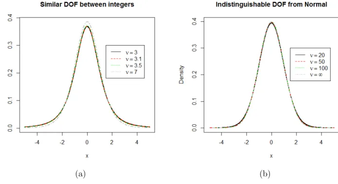
To minimize the burden of the estimation ofνin equation (12), we used a discretized version of the t-distribution (see22) to estimate ν. Since it is hard to distinguish models in-between two integer degrees-of-freedom, and models with ν > 50 are indistinguishable from the normal model (see figure 1), we consider the set ν ={2.5,3,3.5, . . . ,100}. This approach is expected to produce accurate estimate of ν. Initial values for other parameters are obtained from their corresponding two-step estimator. These estimates are then used as the initial value in the
2 3 4 5 6 7 8 9 10 11 12 13 14 15 16 17 18 19 20 21 22 23 24 25 26 27 28 29 30 31 32 33 34 35 36 37 38 39 40 41 42 43 44 45 46 47 48 49 50 51 52 53 54 55 56 57 58 59 60
likelihood function (12) to minimize the possibility of model convergence to a local maximum. We imputed the missing data using E(Y|x, S? <0) =β0x−σρΛ
ν(−γ0w).
(a) (b)
Figure 1: PDF of t distribution- DOF stands for degrees-of-freedom : (a) with varying ν showing difference between integers are indistinguishable. only ν = 7 differs from others; (b) with varying ν showing ν= 50 can approximate the normal distribution.
4
Simulation study
We compare the performance of the proposed robust alternative method of imputation based on asymptotic (ST) and bootstrap (STB) with the18 two-step imputation method (Tstep). We
also included the Heckman full information maximum likelihood method with the asymptotic (SNM) and bootstrap (SNMB) imputation for control purposes. We first consider simulation settings where the outcome and selection models have bivariate-t error distribution. The outcome equation is Yi? = 0.5 + 1.5x1i + x2i +ε1i, where x1i and x2i
iid
∼ N(0,1) and i = 1, . . . , N = 1000. The impact of exclusion restriction on the proposed method is evaluated with selection equations Si? = 1 +x1i+ 0.2x2i+ 1.5wi+ε2i, wi
iid
∼ N(0,1) for exclusion restriction, and S?
i = 1 +x1i+ 0.2x2i +ε2i without an exclusion restriction. Hence, β0 = (0.5,1.5,1.0), and γ0 = (1,1,0.2,1.5) and (1, 1, 0.2) for selection with and without the exclusion restriction, respectively. The covariates x1i, x2i and wi are independent and are also independent of the error terms ε0i = (ε1i, ε2i). The error terms are generated from bivariate t distribution with
3 4 5 6 7 8 9 10 11 12 13 14 15 16 17 18 19 20 21 22 23 24 25 26 27 28 29 30 31 32 33 34 35 36 37 38 39 40 41 42 43 44 45 46 47 48 49 50 51 52 53 54 55 56 57 58 59 60
degree-of-freedom = 5 and ρ = 0.5. The covariance matrix is Σ = σ
2 ρσ
ρσ 1
!
, where σ = 1. We only observe values of Yi? when Si? >0. About 33% of values are not observed with this exclusion restriction, and about 28% without it.
Although it is, perhaps, more instructive to focus on the use of the robust imputation method on covariates that are subject to sample selection, we first examined the performance of the methods on the imputation of missing outcome data. The following scenarios are considered.
First Scenario- Missingness in outcome
(i) Impact of an exclusion restriction- We used Si? = 1 +x1i + 0.2x2i + 1.5wi +ε2i as the
selection component of the model so that there is an additional variable w not present in the outcome model
(ii) Impact of the no exclusion restriction- We used S?
i = 1 + x1i + 0.2x2i + ε2i as the
selection component of the model. That is, the covariates in the outcome and the selection equations overlaps
(iii) Impact of noise variables as exclusion restriction- We used the model in (ii) with addi-tional three noise variables. Noise variables are variables whose true regression coefficients are zero. These variables are common in prespecified models
(iv) Impact of outliers-We generated the data from a selection model with Gaussian mixture errors of the form (1−p)N2(0,Σ) +pN2(0, kΣ), where k >0, p=0.1 and Σ =
1 ρ ρ 1
!
. The selection equation with the exclusion restriction in (i) is used.
Second Scenario- Missingness in covariates
Simulated data were generated using the regression equationYi = 0.5+1.5x1i+x?2i+σε3i, where
ε3i ∼N(0,1),x1i ∼N(0,1) andσ = 1. The underlying regression equation forx?2i = 1+x1i+ε1i with missingness process S?
i = 0.4 +x1i +ε2i. We generated the errors from a bivariate-t distribution with ν = 5 as above. The observed version of x?
2i has about 40% missing data. We consider ρ= 0 (MAR) and ρ= 0.3 and 0.5 (MNAR).
2 3 4 5 6 7 8 9 10 11 12 13 14 15 16 17 18 19 20 21 22 23 24 25 26 27 28 29 30 31 32 33 34 35 36 37 38 39 40 41 42 43 44 45 46 47 48 49 50 51 52 53 54 55 56 57 58 59 60
(a) (b)
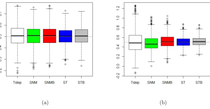
Figure 2: Boxplots for the imputed outcome data : (a) Exclusion restriction; (b) Absence of exclusion restriction.
Simulation results
Figure 2 shows the boxplot of the parameter estimates from the imputed outcome data with or without the exclusion restriction from 1000 simulated data sets. None of the methods is biased under the exclusion restriction (Figure 2a). ST and STB methods are, however, closer to the true parameter and less variable than the methods based on the normal distribution (Tstep, SNM & SNMB). Interestingly, the performance of ST and STB methods in the absence of the exclusion restriction (Figure 2b) are superior to their counterparts under the exclusion restriction. This supported the argument of alleviation of the problem of collinearity adduced for the use of t distribution in sample selection framework by11. The methods based on the
normal distribution are not only biased but highly variable (i.e., imprecise). In particular, the parameter estimates of the outcome under the Tstep method ranges between -0.15 & 1.27 whereas the ST and STB estimates range between 0.22 & 0.87, and 0.23 & 0.86 respectively. Thus, Figure 2 implies the distributional misspecification does not bias the parameter estimates significantly when extra variable predictive of missingness is included in the selection equation of the normal imputation models. The parameter estimates are biased in the absence of an exclusion restriction.
The quest for variables to use for the exclusion restriction criteria to be fulfilled is a daunt-ing exercise in practice. Sometimes, the use of noise variables in the selection equation can
3 4 5 6 7 8 9 10 11 12 13 14 15 16 17 18 19 20 21 22 23 24 25 26 27 28 29 30 31 32 33 34 35 36 37 38 39 40 41 42 43 44 45 46 47 48 49 50 51 52 53 54 55 56 57 58 59 60
(a) (b)
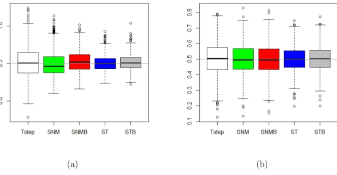
Figure 3: Boxplots for the imputed outcome data : (a) Noise variables as an exclusion restriction; (b) Mixture distribution.
constitute a nuisance in the model estimation. Figure 3a shows that the inclusion of irrele-vant (noise) variables in order to satisfy the exclusion restriction criteria does not make the associated problem go away under the normal models. The Tstep method, although unbiased is highly variable (similar variability as the absence of an exclusion criteria in Figure 2b) pro-viding the most extreme parameter estimates of the response means. ST and STB methods yielded unbiased and low variability results.
The robustness of the proposed imputation method is examined against outliers induced as a result of mixture of normal distributions (Figure 3b). Clearly, both the normal and robust imputation are misspecified. This however, does not appear to bias the parameter estimates (although ST and STB methods are more concentrated near the true parameter). Again, both the ST and STB methods are robust to this misspecification as the estimates are unbiased and show lower variability than the normal models.
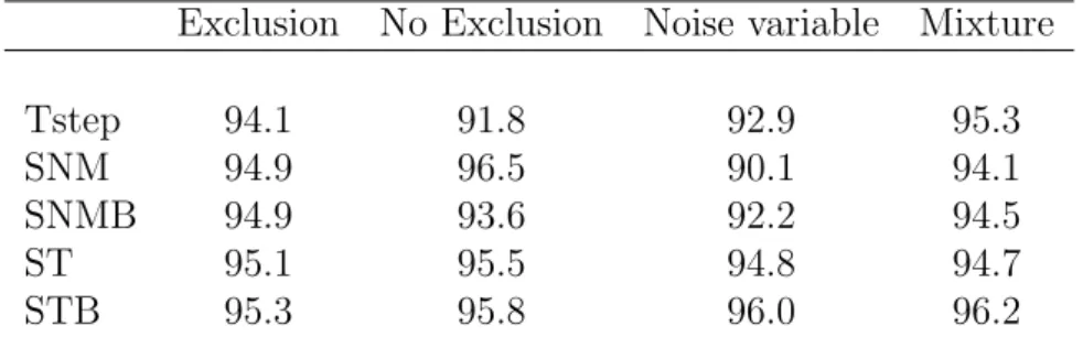
Table 1 shows the coverage of the 95% confidence interval for the parameter estimates using the five imputation methods. The nominal coverage level of 95% is satisfied by the methods for data generated under the exclusion restriction criteria and the mixture distribution. However, the Tstep method shows poor coverage in the absence of the exclusion restriction (91.8%) and noise variables (92.9%). Only the ST and STB methods exhibit satisfactory coverage under these conditions. 2 3 4 5 6 7 8 9 10 11 12 13 14 15 16 17 18 19 20 21 22 23 24 25 26 27 28 29 30 31 32 33 34 35 36 37 38 39 40 41 42 43 44 45 46 47 48 49 50 51 52 53 54 55 56 57 58 59 60
Table 1: 95% confidence interval coverage
Exclusion No Exclusion Noise variable Mixture
Tstep 94.1 91.8 92.9 95.3
SNM 94.9 96.5 90.1 94.1
SNMB 94.9 93.6 92.2 94.5
ST 95.1 95.5 94.8 94.7
STB 95.3 95.8 96.0 96.2
Table 2 shows the results of fitting a normal error regression model using the fully observed variable x1 and partially observedx2. The performance of the models improved asρ increases.
The results also supported the robustness of the ST model.
Table 2: Simulation results for missing covariate data with coefficient of x2 =
1. ρ= 0 represents MAR
ρ= 0 ρ= 0.3 ρ= 0.5
Mean Variance Mean Variance Mean Variance
Tstep 0.956 0.003 0.966 0.003 0.972 0.004 SNM 0.972 0.002 0.982 0.002 0.986 0.003 SNMB 0.974 0.002 0.983 0.002 0.984 0.003 ST 0.981 0.002 0.991 0.002 0.992 0.002 STB 0.980 0.002 0.989 0.002 0.989 0.002
5
Empirical studies
We consider two data examples to illustrate the performance of the robust imputation method. The first data is the ambulatory expenditure from the 2001 Medical Expenditure Panel Survey analyzed by23. The data was also analysed using selection-t model in11. The second application
involves the imputation of the income variable in the 2003-2004 NHANES data. This data was analysed in24, where missing income data was assumed to be missing not at random. We focus on the Tstep, SNM and ST methods since the performance of the bootstrap imputation methods are not too different from the corresponding asymptotic imputation methods.
5.1
Ambulatory expenditure data
The data on ambulatory expenditure contains 3,328 observations of which 526 (15.8%) of the outcome of interest (expenditure) is missing. Apart from expenditure, which is highly skewed,
3 4 5 6 7 8 9 10 11 12 13 14 15 16 17 18 19 20 21 22 23 24 25 26 27 28 29 30 31 32 33 34 35 36 37 38 39 40 41 42 43 44 45 46 47 48 49 50 51 52 53 54 55 56 57 58 59 60
other explanatory variables such as age, gender, education status (educ), ethnicity (blhisp), number of chronic conditions (totchr), insurance status (ins) and income are available in the data. We use log expenditure (lambexp) as the outcome variable due to skewness in line with earlier proposals11,23. The outcome equation, which is usually the model of interest, contains
x = (1, age, f emale, educ, blhisp, totchr, ins) while the selection equation, w = (x, income). Income is included for the exclusion restriction criteria although its use for this purpose is debatable (see11,23). We emphasize that an exclusion restriction is not a necessary condition
for the consistency of the proposed imputation method.
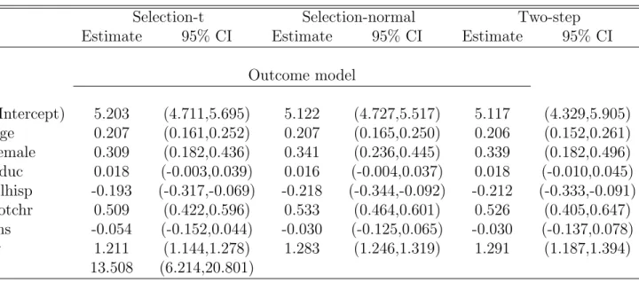
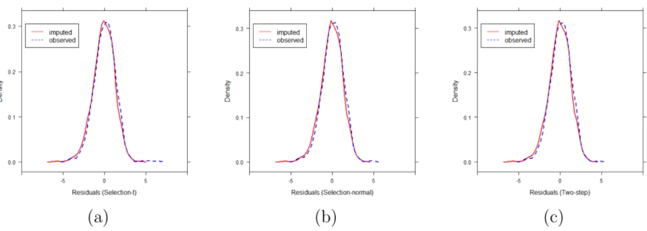
Table 3 shows the results of the robust imputation method and the two alternatives based on the normal distribution. The result is consistent with equivalent results in11, supporting the adequacy of the proposed method. Figure 4 shows the distribution of the residuals of the missing data model. Since the imputation model is correctly specified as an MNAR missingness process, the spread of the residuals of the observed and the imputed data are very similar. Table 3: Estimates from the Outcome model of the Ambulatory expenditure
data after multiple imputation. CI- confidence interval
Selection-t Selection-normal Two-step
Estimate 95% CI Estimate 95% CI Estimate 95% CI
Outcome model (Intercept) 5.203 (4.711,5.695) 5.122 (4.727,5.517) 5.117 (4.329,5.905) age 0.207 (0.161,0.252) 0.207 (0.165,0.250) 0.206 (0.152,0.261) female 0.309 (0.182,0.436) 0.341 (0.236,0.445) 0.339 (0.182,0.496) educ 0.018 (-0.003,0.039) 0.016 (-0.004,0.037) 0.018 (-0.010,0.045) blhisp -0.193 (-0.317,-0.069) -0.218 (-0.344,-0.092) -0.212 (-0.333,-0.091) totchr 0.509 (0.422,0.596) 0.533 (0.464,0.601) 0.526 (0.405,0.647) ins -0.054 (-0.152,0.044) -0.030 (-0.125,0.065) -0.030 (-0.137,0.078) σ 1.211 (1.144,1.278) 1.283 (1.246,1.319) 1.291 (1.187,1.394) ν 13.508 (6.214,20.801)
We also imputed the data under the MAR assumption. That is, we imputed the data using the model specification for the outcome equation. The results are shown in Table 4 Previous analyses of the data posited that all the factors other than the insurance status (ins) are strong predictors of expenditure11. This was supported by the MNAR results in Table 3. The parameter estimates under the MAR assumption are generally larger in magnitude than their MNAR counterparts. Further, two variables (education and insurance status) are not predictors of expenditure under the MAR model. Figure 5 shows kernel density estimates of the imputed and observed expenditure data. There are discrepancies between the densities of the observed and imputed data under the MAR model whereas the densities under the MNAR
2 3 4 5 6 7 8 9 10 11 12 13 14 15 16 17 18 19 20 21 22 23 24 25 26 27 28 29 30 31 32 33 34 35 36 37 38 39 40 41 42 43 44 45 46 47 48 49 50 51 52 53 54 55 56 57 58 59 60
(a) (b) (c)
Figure 4: Distribution of residuals of the missing data model for the outcome data : (a) Selection-t (ST); (b) Selection normal (SNM); (c) Two-step.
Table 4: Imputation of missing outcome in the Ambulatory expenditure data under the MAR assumption. CI- confidence interval
Estimate 95% CI (Intercept) 4.872 (44.536,5.208) age 0.219 (0.174,0.265) female 0.389 (0.291,0.487) educ 0.025 (0.006,0.044) blhisp -0.244 (-0.350,-0.138) totchr 0.569 (0.510,0.627) ins -0.013 (-0.113,0.087) σ 1.181 (1.132,1.231) ν 15.709 (8.054,23.364)
model are similar.
5.2
NHANES data
The US National Health and Nutrition Examination Study (NHANES) is a survey data col-lected by the US National Center for Health Statistics. The survey data dates back to 1999, where individuals of all ages are interviewed in their home annually and complete the health examination component of the survey. The study variables include demographic variables (e.g age and annual household income), physical measurements (e.g. BMI- body mass index), health variables (e.g. diabetes status), and lifestyle variables (e.g. smoking status).
We used NHANES 2003-2004 data to illustrate the methodology of using the robust
im-3 4 5 6 7 8 9 10 11 12 13 14 15 16 17 18 19 20 21 22 23 24 25 26 27 28 29 30 31 32 33 34 35 36 37 38 39 40 41 42 43 44 45 46 47 48 49 50 51 52 53 54 55 56 57 58 59 60
(a) (b)
Figure 5: Kernel density estimates for the marginal distributions of the observed data (blue) and the 10 densities for each imputation for expenditure: (a) MNAR (selection-t); (b) MAR (regression with t-distributed errors).
putation strategy proposed for the imputation of missing covariates (household income) in a model developed to study the effect of socio-economic status on systolic blood pressure (SBP). The data has been used in24 to illustrate the method of subsample ignorable likelihood for
MNAR missing covariates (Income) to study the same effect.24 considered three covariates:
age (in years), gender and BMI, and two socio-economic status variables: income and years of education. We used the same set of variables but added race as additional variable that can predict missingness in household income.
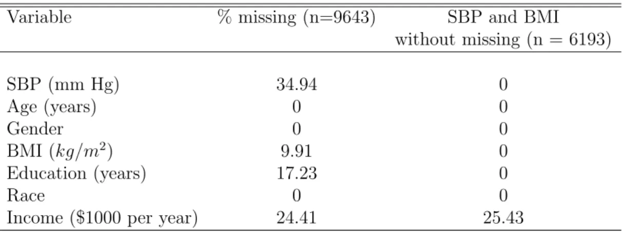
Table 5 shows the percentage of missing data in the variables selected for analysis. Age, gender and race are fully observed, whereas SBP, BMI and household income are subject to missing data. The data analysed is reconstructed such that only income variable has missing data. That is, complete data on SBP and BMI are selected with corresponding measurements on the other variables. This resulted in income having 25.43% misssing data and no missing data on other variables. In principle, there is no need for this as the MICE algorithm allows imputation of multiple missing variables with MAR and MNAR missingness. We focus on income variable in order to evaluate the unalloyed effect of the proposed imputation strategy.
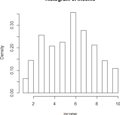
Household income ($1000 per year), was reported as a range of values in dollar (e.g. 0-4999, 5000-9999, etc.) and had 10 interval categories. Figure 6 shows that the ordinal categories of income can be approximated by a continuous distribution. This allows straightforward adaptation of the proposed method without the need for adjustments for ordinal data imputed as continuous data. Education is dichotomized into high school and above versus less than high school and race is treated as categorical variable with 5 levels.
Age, gender, education and race are potential factors that can predict income. These factors
2 3 4 5 6 7 8 9 10 11 12 13 14 15 16 17 18 19 20 21 22 23 24 25 26 27 28 29 30 31 32 33 34 35 36 37 38 39 40 41 42 43 44 45 46 47 48 49 50 51 52 53 54 55 56 57 58 59 60
are also known to lead to selective reporting of income. Therefore, the same set of variables are used in the selection and outcome equations (without exclusion restriction) of the imputation model. Income was imputed using 10 imputations.
Table 5: Percentages of missing data in the NHANES, 2003-2004
Variable % missing (n=9643) SBP and BMI
without missing (n = 6193) SBP (mm Hg) 34.94 0 Age (years) 0 0 Gender 0 0 BMI (kg/m2) 9.91 0 Education (years) 17.23 0 Race 0 0
Income ($1000 per year) 24.41 25.43
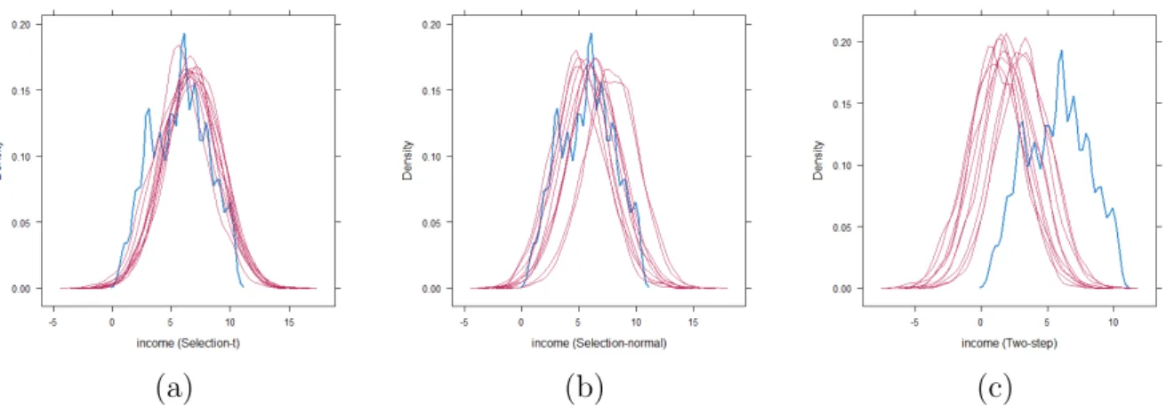
Figure 7 shows kernel density estimates of the imputed and observed income data. The plot based on the selection-t model produces densities of observed and imputed data that match up well. The densities based on the selection normal model are approximately match up (two of the imputed data appears to be shifted away from the observed data). However, there are discrepancies between the densities of the observed and imputed data for the two-step method. A possible explanation for this is the anomalous behavior of the method in the absence of an exclusion restriction, which was also evident from the simulation studies in section 4.
Table 6: Estimates of the effect of socio-economic status on Systolic blood pressure (NHANES, 2003-2004). CI- confidence interval
Selection-t Selection-normal Two-step
Estimate 95% CI Estimate 95% CI Estimate 95% CI
Outcome model (Intercept) 93.173 (91.483,94.863) 92.676 (90.665,94.688) 92.498 (90.694,94.301) age 0.489 (0.470,0.508) 0.558 (0.539,0.577) 0.558 (0.540,0.577) sex (male) -4.362 (-5.022,-3.702) -2.957 (-3.730,-2.184) -2.953 (-3.725,-2.181) education -2.981 (-3.728,-2.234) -3.273 (-4.131,-2.416) -3.283 (-4.127,-2.439) bmi 0.432 (0.376,0.488) 0.382 (0.318,0.447) 0.382 (0.318,0.447) income 0.005 (-0.147,0.156) 0.007 (-0.179,0.192) 0.045 (-0.102,0.193) σ 11.047 (10.689,11.405) 15.462 (15.190,15.735) 15.462 (15.190,15.734) ν 3.782 (3.394,4.171)
Table 6 shows the results of fitting regression models (Selection-t: linear regression with
3 4 5 6 7 8 9 10 11 12 13 14 15 16 17 18 19 20 21 22 23 24 25 26 27 28 29 30 31 32 33 34 35 36 37 38 39 40 41 42 43 44 45 46 47 48 49 50 51 52 53 54 55 56 57 58 59 60
Figure 6: Histogram of ordinal income variable.
student-t errors; Selection-normal and Two-step: OLS regression) to the imputed data sets. The models showed that income is not significantly related to SBP. This observation is anal-ogous to the effect of income in the ignorable likelihood method proposed for the same data in24. The degrees of freedom (ν) in the selection-t model is significant (Estimate = 3.782, CI
= [3.394,4.171]). 2 3 4 5 6 7 8 9 10 11 12 13 14 15 16 17 18 19 20 21 22 23 24 25 26 27 28 29 30 31 32 33 34 35 36 37 38 39 40 41 42 43 44 45 46 47 48 49 50 51 52 53 54 55 56 57 58 59 60
(a) (b) (c)
Figure 7: Kernel density estimates for the marginal distributions of the observed data (blue) and the 10 densities for each imputation for income (red): (a) Selection-t (ST); (b) Selection normal (SNM); (c) Two-step. 3 4 5 6 7 8 9 10 11 12 13 14 15 16 17 18 19 20 21 22 23 24 25 26 27 28 29 30 31 32 33 34 35 36 37 38 39 40 41 42 43 44 45 46 47 48 49 50 51 52 53 54 55 56 57 58 59 60
6
Concluding remarks
This paper proposes the use of selection-t model developed by11 as a robust imputation
al-ternative for missing outcome and covariates data in Heckman-type missing data problem. We have denoted the proposed method as ST and compared it with competing alternatives based on the Heckman’s full information maximum likelihood (SNM) and the two-step (Tstep) method. Contrary to the common notion that MI is valid only under MAR, we have shown that correct specification of the imputation model under MNAR can result in unbiased pa-rameter estimates and valid statistical inference. We have imputed partially observed data by drawing from their conditional distributions using the FCS algorithm. Our proposed imputa-tion method is based on frequentist philosophy (approximate proper imputaimputa-tion) as opposed to the Bayesian (proper) imputation method. The former is easier to use, less computationally intensive and works well in large samples.
Apart from the use of ST method to impute missing covariates data, we have shown its performance for missing outcome data. This was done for two reasons. First, we are able to show that the method performs equally well as its parent sample selection model. Second, the method lends itself naturally to various extensions of the traditional MI techniques (e.g. double robustness concepts can be easily integrated into the imputation model). Specifically, the method can be easily extended to other MNAR imputation models. For instance, instead of the use of imputation modelE(Y|x, S? <0) =β0x−σρΛ
ν(−γ0w), which is similar to the jump to reference approach (see25,26), the imputation approach can also incorporate some form of
pattern mixture-model. That is, the imputation model can be multiplied by a factor or offsets added based on subject matter knowledge.
Two simulation studies were conducted to assess the performance of the ST imputation method in missing outcome and covariates data. The method uniformly outperformed the SNM and Tstep methods in terms of bias and low variance. It attains the nominal coverage level when the missing outcome is imputed under four possible model misspecifications (ab-sence of an exclusion restriction, noise variables, distributional misspecification and outliers). In particular, the ST method performs very well especially in the absence of an exclusion restriction, a problem which has bedeviled the sample selection modelling framework for some time. This attribute is inherited from the parent t model. Basically, for the selection-t model, selection-the inverse Mills raselection-tio is mosselection-tly non-linear over a wide range of iselection-ts supporselection-t. This may also explain the shrinkage effect of the function on the noise variables in the selection process. We emphasize that the good performance of the ST method is not attributable to the data generation process. Figure 8 (Appendix) shows that the ST method still outperforms its competitors even when the data is generated from the normal distribution. The simulation based on covariates data also supported the superiority of the ST method over the SNM and
2 3 4 5 6 7 8 9 10 11 12 13 14 15 16 17 18 19 20 21 22 23 24 25 26 27 28 29 30 31 32 33 34 35 36 37 38 39 40 41 42 43 44 45 46 47 48 49 50 51 52 53 54 55 56 57 58 59 60
Tstep methods.
We analysed two sets of data - Ambulatory expenditure and the 2003-2004 NHANES data sets. The results from the former is comparable with previous analyses in11. The method showed similar fit to the SNM and the Tstep methods. This is, perhaps, due to the exclusion restriction as a result of the omission of income from the outcome equation. However, the advantage of the robust method became pronounced in the imputation of missing covariate (income) in the NHANES data set. We have judged the adequacy of the robust MI method by comparing the distributions of the observed and imputed data. This approach is only valid for the imputation of data that are MAR. Theoretically, the purpose of a reasonably complex imputation model, such as the one proposed here, is to supply sufficient auxiliary variables in appropriate form to make MAR missingness more plausible. As can be seen from Figure 7, the densities of the observed and imputed data are satisfactorily close for the ST method than competing alternatives. This may be due to the absence of an exclusion restriction. It is noteworthy that the use of complete data on systolic blood pressure (SBP) in the NHANES data is for illustrative purposes only. Clearly, missing outcome and covariate data can be accommodated within the MICE imputation algorithm simultaneously.
Another strength of the proposed methodology is that we do not need to fix any value for
ν (the degrees-of-freedom). This can be estimated from data, even when the data is approxi-mately normally distributed. To prevent the likelihood function from possibly converging to a local maximum, we first searched for the values ofν between 2 and 100 that yielded the best fit for the data. This was set as the initial value for ν in the second stage of the maximization of the full log-likelihood function. This may be superfluous in many practical applications. Initial values for other model parameters were obtained from the corresponding two-step method.
Various extensions of the model proposed in section 3 can be formulated. One such extension involves the development of a more flexible imputation model than the method introduced in section 3 using copulas. The use of copulas as alternative modelling framework in selectively reported samples was suggested in10 and further expounded in27. The fact that different
copulas exhibit different dependence patterns offer additional flexibility in its use as imputation model in this setting. The method can readily be extended to impute missing covariates in multilevel sample selection settings16. We are currently investigating methodologies for
obtaining unbiased imputation and variance estimates in this framework.
Finally, although the method we proposed is robust against certain misspecification, it has its limitations, some of which are inherited from the parent selection-t model. For example, the proposed method produced bias estimates when the missingness in a covariate depends on the value of the covariate but conditionally independent of the outcome. Apart from the use of parametric models to achieve robustness, semiparametric and nonparametric sample selection
3 4 5 6 7 8 9 10 11 12 13 14 15 16 17 18 19 20 21 22 23 24 25 26 27 28 29 30 31 32 33 34 35 36 37 38 39 40 41 42 43 44 45 46 47 48 49 50 51 52 53 54 55 56 57 58 59 60
models can be adapted. Ultimately, the guiding principle of any imputation method should be based on the research questions and the use of appropriate sensitivity analysis. The code for the proposed method is available in the Supporting Information.
Acknowledgement
The authors would like to thank the editor and the anonymous referees for the constructive comments, which led to improvements in the manuscript.
Appendix A
(a) (b)
Figure 8: Boxplots for imputed outcome data with normally generated data: (a) Absence of exclusion restriction; (b) Noise variables as exclusion restriction.
2 3 4 5 6 7 8 9 10 11 12 13 14 15 16 17 18 19 20 21 22 23 24 25 26 27 28 29 30 31 32 33 34 35 36 37 38 39 40 41 42 43 44 45 46 47 48 49 50 51 52 53 54 55 56 57 58 59 60
References
[1] Carpenter J, Pocock S, Lamm CJ. Coping with missing data in clinical trials: A model-based approach applied to asthma trials. Stat Med. 2002;21:1043–1066.
[2] Rubin DB. Inference and missing data. Biometrika. 1976;63:581–592.
[3] Moon KG, Donders R, Stijnen T, Harrell FE. Using the outcome for imputation of missing predictor values was preferred. J Clin Epidemiol. 2006;59(10):1092–1101.
[4] White IR, Royston P, Wood AM. Multiple imputation using chained equations: Issues and guidance for practice. Stat Med. 2011;30:377–399.
[5] Van Burren S, Groothuis-Oudshoorn K. mice: Multivariate Imputation by Chained Equa-tions in R. J Stat Softw. 2011;45.
[6] Yuan Y. Sensitivity analysis in multiple imputation for missing data. SAS Institute Inc. 2014;SAS 270–2014.
[7] Van Burren S. Flexible imputation of missing data. Boca Raton: Chapman & Hall, CRC; 2012.
[8] Heckman J. The common structure of statistical models of truncation, sample selection and limited dependent variables and a simple estimator for such models. Ann Econ Soc Meas. 1976;5:475–492.
[9] Heckman J. Sample selection bias as a specification error. Econometrica. 1979;47:153–161. [10] Lee L. Generalized econometric models with selectivity. Econometrica. 1983;51(2):507–
512.
[11] Marchenko YV, Genton MG. A Heckman Selection-t Model. J Am Stat Assoc.
2012;107:304–317.
[12] Ogundimu EO, Hutton JL. A sample selection model with Skew-normal distribution. Scand J Stat. 2016;43:172–190.
[13] Ahn H, Powell JL. Semi-parametric estimation of censored selection models with a non-parametric selection mechanism. J Econometrics. 1993;58:3–29.
[14] Das M, Newwey WK, Vella F. Non-parametric estimation of sample selection models. Rev Econ Stud. 2003;70:33–58.
[15] Vella F. Estimating models with sample selection bias: a survey. J Hum Resour. 1998;33:127–172. 3 4 5 6 7 8 9 10 11 12 13 14 15 16 17 18 19 20 21 22 23 24 25 26 27 28 29 30 31 32 33 34 35 36 37 38 39 40 41 42 43 44 45 46 47 48 49 50 51 52 53 54 55 56 57 58 59 60
[16] Ogundimu EO, Hutton JL. A unified approach to multilevel sample selection model. Commun Stat - Theory Methods. 2016;45:2592–2611.
[17] Copas JB, Li HG. Inference for Non-random Samples. J R Statist Soc B. 1997;59:55–95. [18] Galimard J, Chevret S, Protopopescu C, M Resche-Rigon. A multiple imputation
approach for MNAR mechanisms compatible with Heckman’s model. Stat Med.
2016;35:2907–2920.
[19] Leung SF, Yu S. Collinearity and two-step estimation of sample selection models: prob-lems, origins and remedies. Comput Econ. 2000;15:173–199.
[20] Zhelonkin M, Genton MG, Ronchetti E. Robust inference in sample selection models. J R Statist Soc B. 2016;78:805–827.
[21] Tanner MA, Wong WH. The calculation of posterior distributions by data augmentation (with discussion). J Am Stat Assoc. 1987;82:528–550.
[22] Villa C, Walker SG. Objective Prior for the Number of Degrees of Freedom of a t Distri-bution. Bayesian Analysis. 2014;9(1):197–220.
[23] Cameron AC, Trivedi PK. Microeconometrics using Stata. Revised ed. College Sta-tion,TX: Stata Press; 2010.
[24] Little RJ, Zhang N. Subsample ignorable likelihood for regression analysis with missing data. J R Statist Soc C. 2011;60:591–605.
[25] Little R, Yau L. Intent-to-treat analysis for longitudinal studies with dropouts. Biometrics. 1996;52:1324–1333.
[26] Akacha M, Ogundimu EO. Sensitivity analyses for partially observed recurrent event data. Pharm Stat. 2015;15:4–14.
[27] Smith MD. Modelling sample selection using archimedean copulas. Econometrics Journal. 2003;6:99–123. 2 3 4 5 6 7 8 9 10 11 12 13 14 15 16 17 18 19 20 21 22 23 24 25 26 27 28 29 30 31 32 33 34 35 36 37 38 39 40 41 42 43 44 45 46 47 48 49 50 51 52 53 54 55 56 57 58 59 60
#Supplemental online material for "A robust imputation method for missing #responses and covariates in sample selection models"
# Authors: Emmanuel O. Ogundimu and Gary S. Collins rm(list=ls())
############################################################ #R-codes for selection-t model and imputation
# The code fits a selection-t model
#############################################################
tselectEst<-function (selection,outcome,data = sys.frame(sys.parent()),YS, XS, YO, XO, start=NULL,print.level=0,
maxMethod = "BFGS",...) { if (match("sampleSelection",.packages(),0)==0) require(sampleSelection) if (match("mnormt",.packages(),0)==0) require(mnormt) if (match("mvtnorm",.packages(),0)==0) require(mvtnorm) if (!missing(data)) {
if (!inherits(data, "environment") & !inherits(data, "data.frame") & !inherits(data, "list")) {
stop("'data' must be either environment, data.frame, or list (currently a ",
class(data), ")") }
}
mf <- match.call(expand.dots = FALSE)
m <- match(c("selection", "data", "subset"), names(mf), 0) mfS <- mf[c(1, m)] mfS$drop.unused.levels <- TRUE mfS$na.action <- na.pass mfS[[1]] <- as.name("model.frame") names(mfS)[2] <- "formula" mfS <- eval(mfS, parent.frame()) mtS <- attr(mfS, "terms") XS <- model.matrix(mtS, mfS) YS <- model.response(mfS) YSLevels <- levels(as.factor(YS)) YS <- as.integer(YS == tail(YSLevels, 1)) badRow <- is.na(YS)
badRow <- badRow | apply(XS, 1, function(v) any(is.na(v))) oArg <- match("outcome", names(mf), 0)
m <- match(c("outcome", "data", "subset", "offset"), names(mf), 0) mfO <- mf[c(1, m)] mfO$drop.unused.levels <- TRUE mfO$na.action <- na.pass mfO[[1]] <- as.name("model.frame") names(mfO)[2] <- "formula"
mfO <- eval(mfO, parent.frame()) mtO <- attr(mfO, "terms")
XO <- model.matrix(mtO, mfO) YO <- model.response(mfO)
badRow <- badRow | (is.na(YO) & (!is.na(YS) & YS == 1))
badRow <- badRow | (apply(XO, 1, function(v) any(is.na(v))) & (!is.na(YS) & YS == 1))
if (length(YSLevels) != 2) {
stop("the left hand side of the 'selection' formula\n", "has to contain", " exactly two levels (e.g. FALSE and TRUE)")
}
XS <- XS[!badRow, , drop = FALSE] YS <- YS[!badRow]
XO <- XO[!badRow, , drop = FALSE] YO <- YO[!badRow] 3 4 5 6 7 8 9 10 11 12 13 14 15 16 17 18 19 20 21 22 23 24 25 26 27 28 29 30 31 32 33 34 35 36 37 38 39 40 41 42 43 44 45 46 47 48 49 50 51 52 53 54 55 56 57 58
YO[YS == 0] <- NA XO[YS == 0, ] <- NA loglik <- function(bstart) { p <- ncol(XS); k=ncol(XO) b1 =bstart[1:p];b2 =bstart[(p+1):(k+p)] sigma <- bstart[(k+p+1)] if (sigma < 0) return(NA) rho <- bstart[k+p+2] if ((rho < -1) || (rho > 1)) return(NA) nu <- bstart[k+p+3] ll <- vector() if( nu >2 ){ XS.g <- XS %*% b1 XO.b <- XO %*% b2 u2 <- YO - XO.b r <- sqrt(1 - rho^2) z <- u2/sigma B<- (XS.g + rho/sigma * u2)/r K <- ((nu+1)/(nu+(z^2)))^0.5 K1 <- K*B l1 <- log(dt(z,nu))-log(sigma)+log(pt(K1,nu+1)) ll<- ifelse(YS==0,log(pt(-XS.g,nu)),l1) return(-sum(ll)) } else return(Inf) } if (is.null(start))
tobit2 <- selection(selection,outcome, data=data) coefs <- coef(tobit2, part = "full")
bstart1 <- coefs[tobit2$param$index$betaS] bstart2 <- coefs[tobit2$param$index$betaO] bstart3 <- coefs['sigma'] bstart4 <- coefs['rho'] start <- c(bstart1,bstart2,bstart3,bstart4) startt <- c(start,nu=5) fit <- optim(startt,loglik,control=list(maxit=1000),method="BFGS", hessian=TRUE) loglike <- fit$value nn <- length(YS) nParam <- length(startt) aic <- 2*fit$value + 2*nParam
bic <- 2*fit$value + nParam*log(nn) df <- nn-nParam
N0 <-sum(YS == 0); N1 <- sum(YS == 1);nObs = length(YS) coef <- fit$par vcov <- solve(fit$hessian) hessian <- fit$hessian return(list(coefficients=coef,hessian=hessian,vcov=vcov,level=YSLevels,aic =aic,bic=bic,df=df, loglike=-loglike,N0=N0,N1=N1,NObs=nObs,initial.values=startt)) }
tselect <- function(selection, outcome, data,...) UseMethod("tselect") tselect.default <- function(selection, outcome,data, start = NULL, verbose = FALSE, ...) { mfs <- model.frame(selection, data) mts <- attr(mfs, "terms") 2 3 4 5 6 7 8 9 10 11 12 13 14 15 16 17 18 19 20 21 22 23 24 25 26 27 28 29 30 31 32 33 34 35 36 37 38 39 40 41 42 43 44 45 46 47 48 49 50 51 52 53 54 55 56 57 58
YS <- model.response(mfs, "numeric")
XS <- model.matrix(selection, data = data) mfo <- model.frame(outcome, data)
mto <- attr(mfo, "terms")
YO <- model.response(mfo, "numeric") XO <- model.matrix(outcome, data = data)
est <- tselectEst(selection, outcome, data,start = NULL, verbose = FALSE) co <- est$coefficients
NXS <- ncol(XS) NXO <- ncol(XO) iGamma <- 1:NXS
iBeta <- max(iGamma) + seq(length = NXO) iSigma <- max(iBeta) + 1 iRho <- max(iSigma) + 1 iNu <- max(iSigma) + 2 betaS <- co[iGamma] betaO <- co[iBeta] sigma <- co[iSigma] rho <- co[iRho] nu <- co[iNu] aic <- est$aic bic <- est$bic initial.values <- est$initial.values loglik <- est$loglik est$call <- match.call() class(est) <- "tselect" est } print.tselect <- function(formula, ...) { cat("Call:\n") print(formula$call) cat("\nCoefficients:\n") print(formula$coefficients) } summary.tselect <- function(object, ...) { se <- sqrt(diag(object$vcov)) tval <- coef(object) / se
TAB <- cbind(Estimate = coef(object), StdErr = se,
t.value = tval,
p.value = 2*pt(-abs(tval), df=object$df)) res <- list(call=object$call, coefficients=TAB) class(res) <- "summary.tselect" res } print.summary.tselect <- function(formula, ...) { cat("Call:\n") print(formula$call) cat("\n")
printCoefmat(formula$coefficients, P.value=TRUE, has.Pvalue=TRUE) } 3 4 5 6 7 8 9 10 11 12 13 14 15 16 17 18 19 20 21 22 23 24 25 26 27 28 29 30 31 32 33 34 35 36 37 38 39 40 41 42 43 44 45 46 47 48 49 50 51 52 53 54 55 56 57 58
################################################################# #Imputation code
################################################################# library(mice)
require(sampleSelection)
mice.impute.heckST <- function(y, ry, x,...) {
ry1 <- ry
data <- data.frame(ry1,x,y)
selection <- ry1~ age + female+educ +blhisp+totchr+ins+income outcome <- y~age + female+educ +blhisp+totchr+ins
mle2 <- tselect(selection, outcome, data=data) meane <- coef(mle2)
sig <- solve(mle2$hessian) rv <- t(chol(sig))
b.star <- meane+rv%*%rnorm(ncol(rv)) xo <- model.matrix(outcome, data = data) xs <- model.matrix(selection, data = data) ng <- ncol(xs)
nb <- ncol(xo) igamma <- 1:ng
ibeta <- max(igamma) + seq(length = nb) isigma <- max(ibeta) + 1 irho <- max(isigma) + 1 inu <- max(isigma) + 2 ggamma <- b.star[igamma] beta <- b.star[ibeta] sigma <- b.star[isigma] rho <- b.star[irho] nu <- b.star[inu] nu <- ifelse(nu<=2,3,nu) xb <- xo%*%beta xg <- xs%*%ggamma ivmT <- ((nu+(-xg[!ry,])^2)/(nu-1))*dt(-xg[!ry,],nu)/pt(-xg[!ry,],nu) return(xb[!ry,]-sigma*rho*ivmT+ sigma*rt(sum(!ry),nu)) } ############################################################### # R-codes for fitting the analysis model and combining results ################################################################ ttEst <- function(formula, data,start = NULL, verbose = FALSE){ if (match("gamlss",.packages(),0)==0) require(gamlss)
mf <- model.frame(formula, data) mt <- attr(mf, "terms")
y <- model.response(mf, "numeric") X <- model.matrix(formula, data = data) n <- length(y) k<-ncol(X) tlog <- function(B){ beta <- B[1:k] sigma <- B[k+1] if (sigma < 0) return(NA) nu <- B[k+2] mu <- X%*%beta tempval <- vector() if( nu >2 ){ z <- (y-mu)/sigma tempval <- log(dt(z,nu))-log(sigma) return( -sum(tempval) ) 2 3 4 5 6 7 8 9 10 11 12 13 14 15 16 17 18 19 20 21 22 23 24 25 26 27 28 29 30 31 32 33 34 35 36 37 38 39 40 41 42 43 44 45 46 47 48 49 50 51 52 53 54 55 56 57 58
}
else return(Inf) }
if (is.null(start))
ml1 <- gamlss(formula, data = data,family=TF) ak1 <- coef(ml1) start<- c(ak1,exp(ml1$sigma.coefficients),exp(ml1$nu.coefficients)) options(warn=2) fit <- try(optim(start,fn=tlog,control=list(maxit=1000),method="BFGS", hessian=T)) loglike <- fit$value
nn <- nrow(X); nParam <- length(start) aic <- 2*fit$value + 2*nParam
bic <- 2*fit$value + nParam*log(nn) df <- nn-nParam coef <- fit$par vcov <- solve(fit$hessian) h <- colnames(X); hh <- c(h,"sigma","nu") colnames(vcov) <- rownames(vcov) <- hh names(coef) <- hh
list(coefficients = coef,vcov = vcov,df=df,aic=aic,nu=tail(coef,1), bic=bic,initial.value=start,loglik = -fit$value)
}
tt <- function(formula, ...) UseMethod("tt")
tt.default <- function(formula,data,start = NULL, verbose = FALSE, ...) {
mf <- model.frame(formula, data) mt <- attr(mf, "terms")
y <- model.response(mf, "numeric") X <- model.matrix(formula, data = data)
est <- ttEst(formula, data,start = NULL, verbose = FALSE) co <- est$coefficients
NB <- ncol(X) iBeta <- 1:NB coe <- co[iBeta]
est$fitted.values <- as.vector(X %*%coe) est$residuals <- y - est$fitted.values est$linear.predictors <- est$fitted.values aic <- est$aic bic <- est$bic nu <- est$nu initial.values <- est$initial.values loglik <- est$loglik est$call <- match.call() class(est) <- "tt" est } print.tt <- function(formula, ...) { cat("Call:\n") print(formula$call) cat("\nCoefficients:\n") print(formula$coefficients) } summary.tt <- function(object, ...) { se <- sqrt(diag(object$vcov)) 3 4 5 6 7 8 9 10 11 12 13 14 15 16 17 18 19 20 21 22 23 24 25 26 27 28 29 30 31 32 33 34 35 36 37 38 39 40 41 42 43 44 45 46 47 48 49 50 51 52 53 54 55 56 57 58
tval <- coef(object) / se
TAB <- cbind(Estimate = coef(object), StdErr = se,
t.value = tval,
p.value = 2*pt(-abs(tval), df=object$df)) res <- list(call=object$call, coefficients=TAB) class(res) <- "summary.tt" res } vcov.tt <- function(object){ return(object$vcov) } coef.tt <- function(object){ return(object$coef) }
tt.mids <- function (formula, data, ...) { call <- match.call()
if (!is.mids(data)) stop("The data must have class mids") analyses <- as.list(1:data$m)
for (i in 1:data$m) {
data.i <- complete(data, i)
analyses[[i]] <- tt(formula, data = data.i, ...) }
object <- list(call = call, call1 = data$call,
nmis = data$nmis, analyses = analyses) return(object)
}
pool.impute <- function (object) {
if ((m <- length(object$analyses)) < 2)
stop("At least two imputations are needed for pooling.\n") analyses <- object$analyses
k <- length(coef(analyses[[1]])) names <- names(coef(analyses[[1]]))
qhat <- matrix(NA, nrow = m, ncol = k, dimnames = list(1:m,names)) u <- array(NA, dim = c(m, k, k),
dimnames = list(1:m, names, names)) for (i in 1:m) {
fit <- analyses[[i]] qhat[i, ] <- coef(fit) u[i, , ] <- vcov(fit) }
qbar <- apply(qhat, 2, mean)
ubar <- apply(u, c(2, 3), mean)
e <- qhat - matrix(qbar, nrow = m, ncol = k, byrow = TRUE) b <- (t(e) %*% e)/(m - 1)
t <- ubar + (1 + 1/m) * b r <- (1 + 1/m) * diag(b/ubar) f <- (1 + 1/m) * diag(b/t) df <- (m - 1) * (1 + 1/r)^2
names(r) <- names(df) <- names(f) <- names
fit <- list(call = call, call1 = object$call, call2 = object$call1, nmis = object$nmis, m = m, qhat = qhat, u = u,
2 3 4 5 6 7 8 9 10 11 12 13 14 15 16 17 18 19 20 21 22 23 24 25 26 27 28 29 30 31 32 33 34 35 36 37 38 39 40 41 42 43 44 45 46 47 48 49 50 51 52 53 54 55 56 57 58
qbar = qbar, ubar = ubar, b = b, t = t, r = r, df = df, f = f) return(fit) } summary.impute <- function(object){ est <- object$qbar se <- sqrt(diag(object$t)) tval <- est/se df <- object$df
pval <- 2 * pt(abs(tval), df, lower.tail = FALSE) coefmat <- cbind(est, se, tval, pval)
colnames(coefmat) <- c("Estimate", "Std. Error",
"t value", "Pr(>|t|)") ans <- list( coefficients=coefmat, df=df,
call=object$call1, fracinfo.miss=object$f ) #invisible( ans ) class(ans) <- "summary.impute" ans } print.summary.impute <- function(object) { if (!is.null(object$call1)){ cat("Call: ") dput(object$call1) } cat("\nCoefficients:\n")
printCoefmat(object$coefficients, P.values=T, has.Pvalue=T, signif.legend=T )
cat("\nFraction of information about the coefficients
missing due to nonresponse:","\n") print(object$f)
}
##################################################################### # Ambulatory expenditure example
################################################################# library(ssmrob) data(MEPS2001)#3328 dat <- MEPS2001 lambexp <- dat$lambexp dambexp <- dat$dambexp age <- dat$age female <- dat$female educ <- dat$educ blhisp <- dat$blhisp totchr <- dat$totchr ins <- dat$ins income <- dat$income dd <- data.frame(lambexp,dambexp,age,female,educ,blhisp,totchr,ins,income) #Imputation
ab <- mice(dd, m = 10, seed = 1234,method=c("heckST", "", "", "","","","","",""))
# Results combination across imputed data sets
3 4 5 6 7 8 9 10 11 12 13 14 15 16 17 18 19 20 21 22 23 24 25 26 27 28 29 30 31 32 33 34 35 36 37 38 39 40 41 42 43 44 45 46 47 48 49 50 51 52 53 54 55 56 57 58
fit <- tt.mids(lambexp ~ age + female+educ +blhisp+totchr+ins, data=ab) ak <- pool.impute(fit) nam <- summary.impute(ak) 2 3 4 5 6 7 8 9 10 11 12 13 14 15 16 17 18 19 20 21 22 23 24 25 26 27 28 29 30 31 32 33 34 35 36 37 38 39 40 41 42 43 44 45 46 47 48 49 50 51 52 53 54 55 56 57 58