Regensburger
DISKUSSIONSBEITRÄGE
zur Wirtschaftswissenschaft
University of Regensburg Working Papers in Business,
Economics and Management Information Systems
A hat matrix for monotonicity constrained B-spline
and P-spline regression
Kathrin Kagerer
March, 05 2015
Nr. 484
JEL Classification:
C14, C52
A hat matrix for monotonicity constrained B-spline
and P-spline regression
Kathrin Kagerer∗
March 5, 2015
Summary. Splines constitute an interesting way to flexibly estimate a nonlinear
re-lationship between several covariates and a response variable using linear regression techniques. The popularity of splines is due to their easy application and hence the low computational costs since their basis functions can be added to the regression model like usual covariates. As long as no inequality constraints and penalties are imposed on the estimation, the degrees of freedom of the model estimation can be determined straightforwardly as the number of estimated parameters. This paper derives a for-mula for computing the hat matrix of a penalized and inequality constrained splines estimator. Its trace gives the degrees of freedom of the model estimation which are necessary for the calculation of several information criteria that can be used e.g. for specifying the parameters for the spline or for model selection.
Key words. Spline, monotonicity, penalty, hat matrix, regression, Monte Carlo
sim-ulation.
∗
Most of the work was done as research assistant at the Chair of Econometrics, Faculty of Business, Eco-nomics and Management Information Systems, University of Regensburg, 93040 Regensburg, Germany.
1 Introduction
Compared to classical parametric models, nonparametric models have the advantage of a
flexible functional form that is determined by the available data. With increasing comput-ing power the opportunities for nonparametric methods have improved and hence these
methods are applied more and more. Though estimating models with a spline component basically corresponds to estimating a linear model, optimization methods are required
when inequality constraints such as monotonicity are incorporated. Further, for estimat-ing spline models with monotonicity constraints, the degrees of freedom of the estimated
model are not equal to the number of estimated parameters like it is for non-constrained parametric models. The degrees of freedom of a model estimation are required for example
when information criteria like the Akaike or Schwarz criterion are applied for model se-lection. In this paper, a formula is presented to calculate the hat matrix of the estimated
spline regression with monotonicity constraints and with or without additional penalty terms. The trace of this hat matrix then gives the degrees of freedom of the estimation
like in Ruppert et al. (2003).
The remainder of this paper is organized as follows: Section 2 summarizes the splines specifications used in this paper and derives for each the hat matrix / smoothing matrix.
In a Monte Carlo study, the hat matrix is computed for estimations for data from different DGPs in Section 3 and an empirical example using the LIDAR data set is presented in
Section 4. Section 5 concludes.
2 Splines and their hat matrix
2.1 Splines with penalties and monotonicity constraints
A spline can be used to approximate other functions (e.g. Ruppert et al., 2003, de Boor,
2001, or Dierckx, 1993 as general references for splines). It consists of piecewise polynomial functions which are connected at knots and satisfy certain continuity conditions at these
knots. The order of the piecewise polynomial functions is determined by the order k of the spline. The knot sequenceκ= (κ−(k−1), . . . , κm+k) consists ofm+ 2knon-decreasing
knot positions κj,j =−(k−1), . . . , m+k, where κ0 and κm+1 are the boundary knots
that usually coincide with the bounds of the interval of interest, i.e. in the case of a scalar covariatex these areκ = min(x) and κ = max(x ). A splinescan be constructed
as a linear combination of basis functions. Using B-spline basis functionsBjκ,k, the spline is s(·) = m X j=−(k−1) αjBjκ,k(·). (1)
For a definition of the B-spline basis functions see e.g. de Boor (2001, Chapter IX) or
Schumaker (1981, Chapter 3). Each of the basis functionsBjκ,k is positive on the interval (κj, κj+k) and zero outside and the unweighted sum of the B-spline basis functions (i.e.
αj = 1 for all j) is 1 on [κ0, κm+1].
For regression purposes, splines can be used to estimate an unknown sufficiently
smooth regression curve. Consider the bivariate functional relationship y = f(x) +u with
E(y|x) =f(x), (2)
where the regression functionf is to be estimated using spline regression, i.e. minimizing
n X i=1 yi−f˜(xi) 2 = n X i=1 yi− m X j=−(k−1) ˜ αjBjκ,k(xi) 2 (3)
with respect to them+kparameters ˜αj for a given samplei= 1, . . . , n.
Restricting the estimated parameters ˆαj such that they are in non-decreasing order,
ˆ
αj ≤αˆj+1, j =−(k−1), . . . , m−1, (4)
ensures a monotone increasing estimated spline function and analogously, a decreasing function results for non-increasing parameters (e.g. Dierckx, 1993, Section 7.1). Fork≥4,
this restriction is not necessary to obtain a monotone function, but it is a sufficient con-dition and is easy to implement in the used software.
Cubic splines (k= 4) are commonly used in practice (e.g. Bollaerts et al., 2006, Eilers & Marx, 1996). They are easy to handle, exhibit a good fit and can be subject to several
constraints as for example monotonicity or convexity (cf. Dierckx, 1993, Sections 3.2, 7.1). Hence, cubic splines are also applied here.
Together with the knot sequence, the order of the spline fully determines the functions Bjκ,k of the B-spline basis. Eilers & Marx (1996) and Ruppert et al. (2003, Section 3.4)
location of the knots) which, however, is computationally expensive. But if the knot
sequence is restricted to be equidistant, only the number of knots has to be chosen. Using many knots can result in a rough fit, while using only few knots may not reflect the
conditional relationship (2) well. Hence, Eilers & Marx (1996) propose the use of quite many equidistant knots while penalizing a rough fit (P-splines). This is achieved for
example by avoiding large second-order differences of the estimated parameters ˆαj, i.e.
by penalizing large ∆2α˜j = ˜αj −2 ˜αj−1 + ˜αj−2. The objective function of the resulting
minimization problem then is
n X i=1 yi− m X j=−(k−1) ˜ αjBjκ,k(xi) 2 +λ m X j=−(k−1)+2 (∆2α˜j)2, (5)
whereλis the smoothing parameter which controls the amount of smoothing and has to be chosen by the researcher (see below). Note that for λ = 0 the unpenalized fit as in
Equation (3) results and forλ→ ∞ the fit is given by a straight line fork= 4 (cf. Eilers & Marx, 1996, with cubic splines and a penalty on the second-order differences of the
estimated parameters). Still the number of knots has to be specified, though this is not that influential (see Ruppert et al., 2003, Sections 5.1, 5.5). For example, Ruppert (2002)
proposes to use roughly
min(n/4,35) (6)
inner knots as a rule of thumb.
Now only the smoothing parameterλis left to be specified. It can be chosen for
exam-ple by the (generalized) cross validation criterion (CV, GCV) or the Akaike information criterion (AIC) (e.g. summarized in Ruppert et al., 2003, Section 5.3). Several of these
criteria are based on the elements of the diagonal of the hat matrix of the estimation. Ruppert et al. (2003, Section 3.13) use the trace of the hat matrix of a penalized spline
estimation as the equivalent to the degrees of freedom in linear models. For linear models, the degrees of freedom (df) are given by the number of parameters which in this case
equals the trace of the hat matrix. Section 2.2 explains how to obtain the hat matrix for the spline estimators considered in this section.
For more details on spline estimation using the same notation see Kagerer (2013). That work also covers the general case with one or more than one covariate which is
2.2 A hat matrix for monotonicity constrained P-splines
The hat matrixHof the minimization problem minf˜Pni=1(yi−f˜(xi))2withq×1 covariate
vectorxi is defined to be the matrix for which ˆy=Hy. In case of a linear regression, i.e.
minα˜Pni=1(yi−xiα˜)2, withX=
xT1 · · · xTi · · · xTn
T
, the hat matrix is given by
H=X(XTX)−1XT. (7)
For penalized estimations with a general symmetric penalty matrixD(for an example
see Equation (11) below) wherePn
i=1(yi−xiα˜)2+λα˜TDα˜ is minimized with respect to
˜
α, the hat matrix can be determined as
Hλ =X(XTX+λD)−1XT (8)
(e.g. Ruppert et al., 2003, Section 3.10).
For regression problems with general inequality constraints but without penalty, i.e.
minα˜Pni=1(yi−xiα˜)2 subject toCα˜ ≥0 (for an example see Equation (12) below), the
hat matrix can be derived from the work of Paula (1999) and is given by
Hconstr =X I−(XTX)−1CTR(CR(XTX)−1CTR)−1CR
(XTX)−1XT, (9) where the q×r matrix CR contains ther rows of Csatisfying Cαˆ =0 (cf. Paula, 1993,
1999). Since ˆα is a random variable, it is also random which rows of C satisfyCαˆ =0,
henceCR and with itHconstr and its trace are random. This can also be observed in the
simulation in Section 3 (e.g. Figure 5) and is also discussed in the empirical Section 4.
Penalized estimations with inequality constraints are obtained by minimizingPn
i=1(yi−
xiα˜)2 +λα˜TDα˜ subject to Cα˜ ≥ 0 with respect to ˜α. Since the penalized
estima-tion without constraints can be interpreted as ordinary least-squares problem with X∗ =
XT √λ(D1/2)T
T
and y∗ =yT 0T
T
(e.g. Eilers & Marx, 1996), these two hat
ma-trices can be combined, resulting in the hat matrix for inequality constrained penalized estimations:
Hλ,constr =X I−(XTX+λD)−1CTR(CR(XTX+λD)−1CTR)−1CR
(XTX+λD)−1XT. (10)
Note that for the hat matrices from the constrained estimations (9) and (10), CR is
empty if the inequality constraint on Cαˆ is not necessary (i.e. none of the entries ofCαˆ
Applying the properties of the trace operator, the trace of the hat matrix reduces to
q(i.e. the number of estimated parameters) in case of the unconstrained unpenalized esti-mation (hat matrix (7)) and toq−rin case of the constrained but unpenalized estimation
(hat matrix (9)). Hence for minα˜ Pni=1(yi−xiα˜)2 subject to Cα˜ ≥ 0, the degrees of
freedom of the estimation equal the number of estimated parameters minus the number
of rows of the constraint matrix C for which Cαˆ = 0 holds. For the case of penalized estimations, the trace of the hat matrices (8) and (10) can not be simplified in an analog
way and have to be determined after having estimated the model with the given data.
For penalized monotonicity constrained spline estimations ((5) with constraint (4)) with equidistant knots for a scalar covariatex, the (i, j)-th entry of then×(m+k) matrixX
isBκj−,kk(xi). The penalty matrixDis the matrix for whichPmj=−(k−1)+2(∆2α˜j)2 = ˜αTDα˜
holds and hence is given by
D= 1−2 1 −2 5−4 1 1−4 6−4 · 1−4 6 · · 1−4 · · 1 1 · · −4 1 · · 6−4 1 · −4 5−2 1−2 1 . (11)
Note that the penalty matrix can also be obtained for non-equidistant knot sequences (cf.
Kagerer, 2013).
The constraint matrix C required to satisfy the constraint (4) which results in a monotonically increasing fit is
C= −1 1 −1 1 −1 1 ... ... (12)
and for a monotone decreasing fit it has to be multiplied by−1.
3 Monte Carlo simulation
3.1 Data generating processes
In this section only bivariate data generating processes (DGPs) are considered, i.e.
y=f(x) +u.
For all DGPs, the scalar covariate xand the errors u are assumed to be distributed as
To be able to use the same knot sequence for all replications, x is rescaled such that
mini(xi) = 0 and maxi(xi) = 1 for each sample.
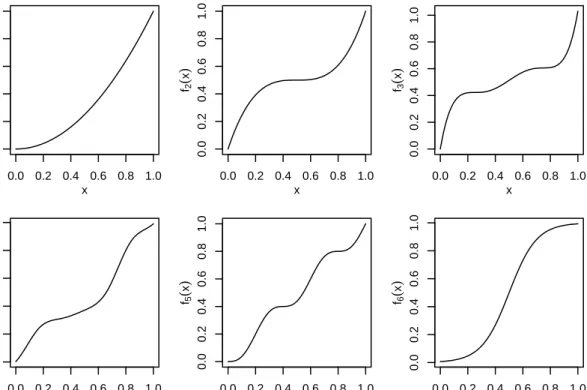
Six different regression functionsf are studied:
f1(x) =x2, f2(x) = 4 (x−0.5)3+ 0.5, f3(x) = 34.1x5−85.3x4+ 78.23x3−32x2+ 6x, f4(x) = 5 X j=−3 αjBjκ,4(x)−0.2 forαT = 2 2 7 7 8 9 16 16 20/14, f5(x) =x−sin(5π x)/16, f6(x) = exp(10(x−0.5)) 1 + exp(10(x−0.5)).
The functions f1, f2 and f3 are polynomial functions of different degrees, f4 is a cubic
spline, f5 is the sine function with higher periodicity and a trend and f6 is the CDF of
the logistic distribution with parameters a = 0.5 and b = 0.1. All functions are chosen such that they are monotonically increasing on the interval [0,1]. Further, they are
(ap-proximately) scaled on the interval [0,1], i.e. f(x) ∈ [0,1] for x ∈ [0,1], hence the same error variance σ2 is appropriate for all DGPs and is chosen to equal σ2 = 0.09. Figure 1 presents the respective functions and Figure 2 shows one simulated sample for each DGP.
For all estimations the open source software R (R Core Team, 2014, version 3.1.2,
32 bit) is used. The spline regressions are based on the base package splines and the constraint is implemented using the function pcls from the mgcv package from Wood
(2014).
3.2 Simulation results
For each replicationr = 1, . . . , R, R = 1000, of the Monte Carlo simulation, a sample of size n = 500 is drawn for x and u and the corresponding y for the regression functions
f1 tof6 are calculated. According to Equation (6), the knot sequence for the spline basis
κ contains m = 35 equidistant inner knots and is subject to the constraint (4) for all
functions f1 to f6. For each function the smoothing parameter λ has to be chosen. In
the simulation the true functionf is known. Hence,λ can be selected for each of the six
0.0 0.2 0.4 0.6 0.8 1.0 0.0 0.2 0.4 0.6 0.8 1.0 x f1 ( x ) 0.0 0.2 0.4 0.6 0.8 1.0 0.0 0.2 0.4 0.6 0.8 1.0 x f2 ( x ) 0.0 0.2 0.4 0.6 0.8 1.0 0.0 0.2 0.4 0.6 0.8 1.0 x f3 ( x ) 0.0 0.2 0.4 0.6 0.8 1.0 0.0 0.2 0.4 0.6 0.8 1.0 x f4 ( x ) 0.0 0.2 0.4 0.6 0.8 1.0 0.0 0.2 0.4 0.6 0.8 1.0 x f5 ( x ) 0.0 0.2 0.4 0.6 0.8 1.0 0.0 0.2 0.4 0.6 0.8 1.0 x f6 ( x )
Figure 1: Plot of the regression functions of each DGP used in the simulation.
● ● ● ● ● ● ● ● ● ● ● ● ● ● ● ● ● ● ● ● ● ● ● ● ● ● ● ● ● ● ● ● ● ● ● ● ● ● ● ● ● ● ● ● ● ● ● ● ● ● ● ● ● ● ● ● ● ● ● ● ● ● ● ● ● ● ● ● ● ● ● ● ● ● ● ● ● ● ● ● ● ● ● ● ● ● ● ● ● ● ● ● ● ● ● ● ● ● ● ● ● ● ● ● ●● ● ● ● ● ● ● ● ● ● ● ● ● ● ● ● ● ● ● ● ● ● ● ● ● ● ● ● ● ● ● ● ● ● ● ● ● ● ● ● ● ● ● ● ● ● ● ● ● ● ● ● ● ● ● ● ● ● ● ● ● ● ● ● ● ● ● ● ● ● ● ● ● ● ● ● ● ● ● ● ● ● ● ● ● ● ● ● ● ● ●● ● ● ● ● ● ● ● ● ● ● ● ● ● ● ● ● ● ● ● ● ● ● ● ● ● ● ● ● ● ● ● ● ● ● ● ● ● ● ● ● ● ● ● ● ● ● ● ● ● ● ● ● ● ● ● ● ● ● ● ● ● ● ● ● ● ● ● ● ● ● ● ● ● ● ● ● ● ● ● ● ● ● ● ● ● ● ● ● ● ● ● ● ● ● ● ● ● ● ● ● ● ● ● ● ● ● ● ● ● ● ● ● ● ● ● ● ● ● ● ● ● ● ● ● ● ● ● ● ● ● ● ● ● ● ● ● ● ● ● ● ● ● ● ● ● ● ● ● ● ● ● ● ● ● ● ● ● ● ● ● ● ● ● ● ● ● ● ● ● ● ● ● ● ● ● ● ● ● ● ● ● ● ● ● ● ● ● ● ● ● ● ● ● ● ● ● ● ● ● ● ● ● ● ● ● ● ● ● ● ● ● ● ● ● ● ● ● ●● ● ● ● ● ● ● ● ● ● ● ● ● ● ● ● ● ● ● ● ● ● ● ● ● ● ● ● ● ● ● ● ● ● ● ● ● ● ● ● ● ● ● ● ● ● ● ● ● ● ● ● ● ● ● ● ● ● ● ● ● ● ● ● ● ● ● ● ● ● ● ● ● ● ● ● ● ● ● ● ● ● ● ● ● 0.0 0.2 0.4 0.6 0.8 1.0 −1.0 0.0 1.0 2.0 x y1 ● ● ● ● ● ● ● ● ● ● ● ● ● ● ● ● ● ● ● ● ● ● ● ● ● ● ● ● ● ● ● ● ● ● ● ● ● ● ● ● ● ● ● ● ● ● ● ● ● ● ● ● ● ● ● ● ● ● ● ● ● ● ● ● ● ● ● ● ● ● ● ● ● ● ● ● ● ● ● ● ● ● ● ● ● ● ● ● ● ● ● ● ● ● ● ● ● ● ● ● ● ● ● ● ●● ● ● ● ● ● ● ● ● ● ● ● ● ● ● ● ● ● ● ● ● ● ● ● ● ● ● ● ● ● ● ● ● ● ● ● ● ● ● ● ● ● ● ● ● ● ● ● ● ● ● ● ● ● ● ● ● ● ● ● ● ● ● ● ● ● ● ● ● ● ● ● ● ● ● ● ● ● ● ● ● ● ● ● ● ● ● ● ● ● ● ● ● ● ● ● ● ● ● ● ● ● ● ● ● ● ● ● ● ● ● ● ● ● ● ● ● ● ● ● ● ● ● ● ● ● ● ● ● ● ● ● ● ● ● ● ● ● ● ● ● ● ● ● ● ● ● ● ● ● ● ● ● ● ● ● ● ● ● ● ● ● ● ● ● ● ● ● ● ● ● ● ● ● ● ● ● ● ● ● ● ● ● ● ● ● ● ● ● ● ● ● ● ● ● ● ● ● ● ● ● ● ● ● ● ● ● ● ● ● ● ● ● ● ● ● ● ● ● ● ● ● ● ● ● ● ● ● ● ● ●● ● ● ● ● ● ● ● ● ● ● ● ● ● ● ● ● ● ● ● ● ● ● ● ● ● ● ● ● ● ● ● ● ● ● ● ● ● ● ● ● ● ● ● ● ● ● ● ● ● ● ● ● ● ● ● ● ● ● ● ● ● ● ● ● ● ● ● ● ● ● ● ● ● ● ● ● ● ●● ● ● ● ● ● ● ● ● ● ● ● ● ● ● ●● ● ● ● ● ● ● ● ● ● ● ● ● ● ● ● ● ● ● ● ● ● ● ● ● ● ● ● ● ● ● ● ● ● ● ● ● ● ● ● ● ● ● ● ● ● ● ● ● ● ● ● ● ● ● ● ● ● ● ● ● ● ● ● ● ● ● ● ● 0.0 0.2 0.4 0.6 0.8 1.0 −1.0 0.0 1.0 2.0 x y2 ● ● ● ● ● ● ● ● ●● ● ● ● ● ● ● ● ● ● ● ● ● ● ● ● ● ● ● ● ● ●● ● ● ● ● ● ● ● ● ● ● ● ● ● ● ● ● ● ● ● ● ● ● ● ● ● ● ● ● ● ● ● ● ● ● ● ● ● ● ● ● ● ● ● ● ● ● ● ● ● ● ● ● ● ● ● ● ● ● ● ● ● ● ● ● ● ● ● ● ● ● ● ● ●● ● ● ● ● ● ● ● ● ● ● ● ● ● ● ● ● ● ● ● ● ● ● ● ● ● ● ● ● ● ● ● ● ● ● ● ● ● ● ● ● ● ● ● ● ● ● ● ● ● ● ● ● ● ● ● ● ● ● ● ● ● ● ● ● ● ● ● ● ● ● ● ● ● ● ● ● ● ● ● ● ● ● ● ● ● ● ● ● ● ● ● ● ● ● ● ● ● ● ● ● ● ● ● ● ● ● ● ● ● ● ● ● ● ● ● ● ● ● ● ● ● ● ● ● ● ● ● ● ● ● ● ● ● ● ● ● ● ● ● ● ● ● ● ● ● ● ● ● ● ● ● ● ● ● ● ● ● ● ● ● ● ● ● ● ● ● ● ● ● ● ● ● ● ● ● ● ● ● ● ● ● ● ● ● ● ● ● ● ● ● ● ● ● ● ● ● ● ● ● ● ● ● ● ● ● ● ● ● ● ● ● ● ● ● ● ● ● ● ● ● ● ● ● ● ● ● ● ● ● ● ● ● ● ● ● ● ● ● ● ● ● ● ● ● ● ● ● ● ● ● ● ● ● ● ● ● ● ● ● ● ● ● ● ● ● ● ● ● ● ● ● ● ● ● ● ● ● ● ● ● ● ● ● ● ● ● ● ● ● ● ● ● ● ● ● ● ● ● ● ● ● ● ● ● ● ● ● ● ●● ● ● ● ● ● ● ● ● ● ● ● ● ● ● ●● ● ● ● ● ● ● ● ● ● ● ● ● ● ● ● ● ● ● ● ● ● ● ● ● ● ● ● ● ● ● ● ● ● ● ● ● ● ● ● ● ● ● ● ● ● ● ● ● ● ● ● ● ● ● ● ● ● ● ● ● ● ● ● ● ● ● ● ● 0.0 0.2 0.4 0.6 0.8 1.0 −1.0 0.0 1.0 2.0 x y3 ● ● ● ● ● ● ● ● ● ● ● ● ● ● ● ● ● ● ● ● ● ● ● ● ● ● ● ● ● ● ● ● ● ● ● ● ● ● ● ● ● ● ● ● ● ● ● ● ● ● ● ● ● ● ● ● ● ● ● ● ● ● ● ● ● ● ● ● ● ● ● ● ● ● ● ● ● ● ● ● ● ● ● ● ● ● ● ● ● ● ● ● ● ● ● ● ● ● ● ● ● ● ● ● ●● ● ● ● ● ● ● ● ● ● ● ● ● ● ● ● ● ● ● ● ● ● ● ● ● ● ● ● ● ● ● ● ● ● ● ● ● ● ● ● ● ● ● ● ● ● ● ● ● ● ● ● ● ● ● ● ● ● ● ● ● ● ● ● ● ● ● ● ● ● ● ● ● ● ● ●● ● ● ● ● ● ● ● ● ● ● ● ● ● ● ● ● ●● ● ● ● ● ● ● ● ● ● ● ● ● ● ● ● ● ● ● ● ● ● ● ● ● ● ● ● ● ● ● ● ● ● ● ● ● ● ● ● ● ● ● ● ● ● ● ● ● ● ● ● ● ● ● ● ● ● ● ● ● ● ● ● ● ● ● ● ● ● ● ● ● ● ● ● ● ● ● ● ● ● ● ● ● ● ● ● ● ● ● ● ● ● ● ● ● ● ● ● ● ● ● ● ● ● ● ● ● ● ● ● ● ● ● ● ● ● ● ● ● ● ● ● ● ● ● ● ● ● ● ● ● ● ● ● ● ● ● ● ● ● ● ● ● ● ● ● ● ● ● ● ● ● ● ● ● ● ● ● ● ● ● ● ● ● ● ● ● ● ● ● ● ● ● ● ● ● ● ● ● ● ● ● ● ● ● ● ● ● ● ● ● ● ● ● ● ● ● ● ● ● ● ● ● ● ● ● ● ● ● ● ● ● ● ●● ● ● ● ●● ● ● ● ● ● ● ● ● ● ●● ● ● ● ● ● ● ● ● ● ● ● ● ● ● ● ● ● ● ● ● ● ● ● ● ● ● ● ● ● ● ● ● ● ● ● ● ● ● ● ● ● ● ● ● ● ● ● ● ● ● ● ● ● ● ● ● ● ● ● ● ● ● ● ● ● ● ● ● 0.0 0.2 0.4 0.6 0.8 1.0 −1.0 0.0 1.0 2.0 x y4 ● ● ● ● ● ● ● ● ● ● ● ● ● ● ● ● ● ● ● ● ● ● ● ● ● ● ● ● ● ● ●● ● ● ● ● ● ● ● ● ● ● ● ● ● ● ● ● ● ● ● ● ● ● ● ● ● ● ● ● ● ● ● ● ● ● ● ● ● ● ● ● ● ● ● ● ● ● ● ● ● ● ● ● ● ● ● ● ● ● ● ● ● ● ● ● ● ● ● ● ● ● ● ● ●● ● ● ● ● ● ● ● ● ● ● ● ● ● ● ● ● ● ● ● ● ● ● ● ● ● ● ● ● ● ● ● ● ● ● ● ● ● ● ● ● ● ● ● ● ● ● ● ● ● ● ● ● ● ● ● ● ● ● ● ● ● ● ● ● ● ● ● ● ● ● ● ● ● ● ●● ● ● ● ● ● ● ● ● ● ● ● ● ● ● ● ● ● ● ● ● ● ● ● ● ● ● ● ● ● ● ● ● ● ● ● ● ● ● ● ● ● ● ● ● ● ● ● ● ● ● ● ● ● ● ● ● ● ● ● ● ● ● ● ● ● ● ● ● ● ● ● ● ● ● ● ● ● ● ● ● ● ● ● ● ● ● ● ● ● ● ● ● ● ● ● ● ● ● ● ● ● ● ● ● ● ● ● ● ● ● ● ● ● ● ● ● ● ● ● ● ● ● ● ● ● ● ● ● ● ● ● ● ● ● ● ● ● ● ● ● ● ● ● ● ● ● ● ● ● ● ● ● ● ● ● ● ● ● ● ● ● ● ● ● ● ● ● ● ● ● ● ● ● ● ● ● ● ● ● ● ● ● ● ● ● ● ● ● ● ● ● ● ● ● ● ● ● ● ● ● ● ● ● ● ● ● ● ● ● ● ● ● ● ● ● ● ● ● ● ● ● ● ● ● ● ● ● ● ● ● ● ● ●● ● ● ● ●● ● ● ● ● ● ● ● ● ● ● ● ● ● ● ● ● ● ● ● ● ● ● ● ● ● ● ● ● ● ● ● ● ● ● ● ● ● ● ● ● ● ● ● ● ● ● ● ● ● ● ● ● ● ● ● ● ● ● ● ● ● ● ● ● ● ● ● ● ● ● ● ● ● ● ● ● ● ● ● 0.0 0.2 0.4 0.6 0.8 1.0 −1.0 0.0 1.0 2.0 x y5 ● ● ● ● ● ● ● ● ● ● ● ● ● ● ● ●● ● ● ● ● ● ● ● ● ● ● ● ● ● ●● ● ● ● ● ● ● ● ● ● ● ● ● ● ● ● ● ● ● ● ● ● ● ● ● ● ● ● ● ● ● ● ● ● ● ● ● ● ● ● ● ● ● ● ● ● ● ● ● ● ● ● ● ● ● ● ● ● ● ● ● ● ● ● ● ● ● ● ● ● ● ● ● ●● ● ● ● ● ● ● ● ● ● ● ● ● ● ● ● ● ● ● ● ● ● ● ● ● ● ● ● ● ● ● ● ● ● ● ● ● ● ● ● ● ● ● ● ● ● ● ● ● ● ● ● ● ● ● ● ● ● ● ● ● ● ● ● ● ● ● ● ● ● ● ● ● ● ● ●● ● ● ● ● ● ● ● ● ● ● ● ● ● ● ● ● ● ● ● ● ● ● ● ● ● ● ● ● ● ● ● ● ● ● ● ● ● ● ● ● ● ● ● ● ● ● ● ● ● ● ● ● ● ● ● ● ● ● ● ● ● ● ● ● ● ● ● ● ● ● ● ● ● ● ● ● ● ● ● ● ● ● ● ● ● ● ● ● ● ● ● ● ● ● ● ●● ● ● ● ● ● ● ● ● ● ● ● ● ● ● ● ● ● ● ● ● ● ● ● ● ● ● ● ● ● ● ● ● ● ● ● ● ● ● ● ● ● ● ● ● ● ● ● ● ● ● ● ● ● ● ● ● ●● ● ● ● ● ● ● ● ● ● ● ● ● ● ● ● ● ● ● ● ● ● ● ● ● ● ● ● ● ● ● ● ● ● ● ● ● ● ● ● ● ● ● ● ● ● ● ● ● ● ● ● ● ● ● ● ● ● ● ● ● ● ● ● ● ● ● ● ● ● ● ● ● ● ● ● ● ● ●● ● ● ● ● ● ● ● ● ● ● ● ● ● ● ● ● ● ● ● ● ● ● ● ● ● ● ● ● ● ● ● ● ● ● ● ● ● ● ● ● ● ● ● ● ● ● ● ● ● ● ● ● ● ● ● ● ● ● ● ● ● ● ● ● ● ● ● ● ● ● ● ● ● ● ● ● ● ● ● ● ● ● ● ● 0.0 0.2 0.4 0.6 0.8 1.0 −1.0 0.0 1.0 2.0 x y6
Then the smoothing parameter is chosen as λ= arg min ˜ λ 1 R R X r=1 1 n n X i=1 f(xi,r)−fˆλ,r˜ (xi,r) 2 ! ,
wherexi,ris theith observation in therth replication and ˆf˜λ,r is the estimate off for the
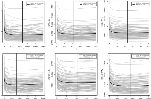
rth replication and a given value ˜λfor the smoothing parameter. The results forλchosen by minimizing theM ISE can be found in Figure 3 and are comparable to the smoothing
parameter analogously obtained by the meanGCV or the mean AIC criterion (cf. Table 1). Selection criteria like GCV or AIC are feasible for real data problems when f is
unknown and hence are applied for the empirical example in Section 4. The advantage of using theM ISE for the simulation is that it does not contain the trace of the hat matrix
of the estimations and hence can be used to compare the results to those for e.g.GCV or AIC. Note that for choosing the optimal λin the simulation, only 100 of the R = 1000
samples are included to reduce the computational effort.
0 2000 4000 6000 8000 10000 0.000 0.001 0.002 0.003 λ ISE( λ ) f or f 1
ISE(λ), for 100 samples MISE(λ), λopt=4700 0 200 400 600 800 1000 0.000 0.001 0.002 0.003 0.004 λ ISE( λ ) f or f 2
ISE(λ), for 100 samples MISE(λ), λopt=420 0 20 40 60 80 100 0.001 0.002 0.003 0.004 0.005 λ ISE( λ ) f or f 3
ISE(λ), for 100 samples MISE(λ), λopt=46 0 200 400 600 800 1000 0.000 0.001 0.002 0.003 0.004 λ ISE( λ ) f or f 4
ISE(λ), for 100 samples MISE(λ), λopt=320 0 50 100 150 200 0.001 0.002 0.003 λ ISE( λ ) f or f 5
ISE(λ), for 100 samples MISE(λ), λopt=104 0 200 400 600 800 1000 0.000 0.001 0.002 0.003 λ ISE( λ ) f or f 6
ISE(λ), for 100 samples MISE(λ), λopt=530
Figure 3: Integrated squared error from 100 of the R = 1000 samples (ISE, grey) and mean integrated squared error (M ISE, black) depending onλ.
function f1 f2 f3 f4 f5 f6
λopt from M ISE 4700 420 46 320 104 530
λopt from GCV 5100 620 43 360 120 490
λopt from AIC 4400 620 30 360 120 490
Table 1: Optimalλfor the different regression functions chosen with respect toM ISE, meanGCV and meanAIC from 100 of theR= 1000 samples.
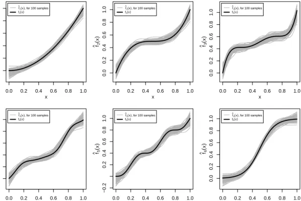
For each of the R= 1000 samples, the six functions are estimated using cubic splines
with m = 35 inner knots, the optimal smoothing parameter λ with respect to M ISE and monotonicity constraint (4). The corresponding estimated regression curves can be
regarded in Figure 4 where it can be observed that they fit the DGP functions very well. Therefore, the smoothing parameters appear to be well-chosen.
0.0 0.2 0.4 0.6 0.8 1.0 0.0 0.2 0.4 0.6 0.8 1.0 x f ^(1 x ) f ^1(x), for 100 samples f1(x) 0.0 0.2 0.4 0.6 0.8 1.0 0.0 0.2 0.4 0.6 0.8 1.0 x f ^ (2 x ) f ^2(x), for 100 samples f2(x) 0.0 0.2 0.4 0.6 0.8 1.0 0.0 0.2 0.4 0.6 0.8 1.0 x f ^(3 x ) f ^3(x), for 100 samples f3(x) 0.0 0.2 0.4 0.6 0.8 1.0 0.0 0.2 0.4 0.6 0.8 1.0 x f ^(4 x ) f ^4(x), for 100 samples f4(x) 0.0 0.2 0.4 0.6 0.8 1.0 −0.2 0.2 0.4 0.6 0.8 1.0 x f ^ (5 x ) f ^5(x), for 100 samples f5(x) 0.0 0.2 0.4 0.6 0.8 1.0 0.0 0.2 0.4 0.6 0.8 1.0 x f ^(6 x ) f ^6(x), for 100 samples f6(x)
Figure 4: Fitted regression curves from 100 of the R = 1000 samples and corresponding DGP function. For each estimation the same optimalλw.r.t.M ISE (see Table 2) is used.
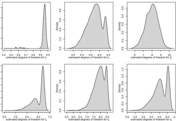
Using the estimation results, the hat matrix (10) and its trace are calculated each time. The results are aggregated in the density plots in Figure 5. It can be seen that
for each DGP the obtained degrees of freedom do not vary by much (compared to the
maximal degrees of freedom ofm+k= 39) and the estimated standard errors lie between 0.08 and 0.70 for the six chosen functions (cf. also Table 2). For the polynomial functions
f1,f2 andf3 of degree 2, 3 and 5 (i.e. at most 3, 4, 6 parameters to estimate) the degrees
of freedom are about 4, 5-6 and 7-9, hence only slightly overestimated. Note that the
extent of over-/underestimation of the degree of the functions also depends on the chosen error variance. For example a larger error variance ofσu2 = 0.25 leads to traces of the hat matrix of 3-4, 4-5 and 6-7 for these three functions, which is also quite close to the degrees of the three polynomial functions.
3.4 3.5 3.6 3.7 3.8 3.9 4.0 0 5 10 15 20
estimated degrees of freedom for f1
Density 4.5 5.0 5.5 6.0 6.5 0.0 0.2 0.4 0.6 0.8
estimated degrees of freedom for f2
Density 6 7 8 9 10 0.0 0.1 0.2 0.3 0.4 0.5
estimated degrees of freedom for f3
Density 5.0 5.5 6.0 6.5 7.0 0.0 0.5 1.0 1.5 2.0 2.5 3.0 3.5
estimated degrees of freedom for f4
Density 5.5 6.0 6.5 7.0 7.5 8.0 8.5 0.0 0.2 0.4 0.6 0.8
estimated degrees of freedom for f5
Density 3.5 4.0 4.5 5.0 5.5 6.0 6.5 0.0 0.2 0.4 0.6 0.8 1.0 1.2
estimated degrees of freedom for f6
Density
Figure 5: Density plot of the degrees of freedom of the estimations for the R = 1000 simulated samples. For each estimation the same optimal λw.r.t.M ISE (see Table 2) is used.
The selection of the optimal smoothing parameter λ is mostly guided by selection
criteria, but these often depend on the hat matrix or functions of its elements (e.g.AIC). This was not the case in the simulation since λ was selected by minimizing the M ISE.
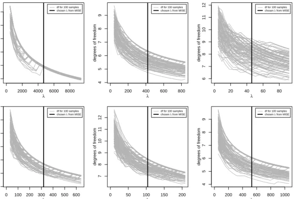
Figure 6 shows the dependence of the trace of the hat matrix of the estimated model from the selected smoothing parameter. The vertical line corresponds to the optimal λ
function f1 f2 f3 f4 f5 f6
min 3.4 4.4 5.8 5.2 5.8 3.9
max 4.0 6.4 10.0 6.8 8.5 6.1
mean 3.9 5.7 8.0 6.5 7.9 5.6
sd 0.08 0.42 0.70 0.27 0.43 0.43
Table 2: Sample minimum, maximum, mean and standard deviation of the traces of the hat ma-trices for the different DGPs from theR= 1000 samples.
according toM ISE.
For increasing λ the degrees of freedom of the estimation decreases as was to be expected since the fitted curve converges to a straight line (cf. Eilers & Marx, 1996). Note
that if the plot was drawn further toλ→ ∞, the degrees of freedom would converge to 2 corresponding to a straight line with a non-zero slope (cf. Section 2.1).
0 2000 4000 6000 8000 3.5 4.0 4.5 5.0 5.5 6.0 λ degrees of freedom df for 100 samples chosen λ from MISE
0 200 400 600 800 4 5 6 7 8 9 λ degrees of freedom df for 100 samples chosen λ from MISE
0 20 40 60 80 6 7 8 9 10 11 12 λ degrees of freedom df for 100 samples chosen λ from MISE
0 100 200 300 400 500 600 5 6 7 8 9 10 11 λ degrees of freedom df for 100 samples chosen λ from MISE
0 50 100 150 200 7 8 9 10 11 12 λ degrees of freedom df for 100 samples chosen λ from MISE
0 200 400 600 800 1000 4 5 6 7 8 9 λ degrees of freedom df for 100 samples chosen λ from MISE
Figure 6: Degrees of freedom of the estimations depending on the smoothing parameterλfor 100 of theR= 1000 samples.
4 Empirical example
In the following, the well-known data set containing LIDAR data is analyzed.
The LIDAR (light detection and ranging) data set which has been examined
es-pecially with nonparametric techniques (e.g. Ruppert et al., 2003, Ruppert & Carroll, 2000) can be found on the homepage of the book of Ruppert et al. (2003,http://stat.
tamu.edu/~carroll/semiregbook/). The data set includes information on n= 221 ob-servations from a LIDAR experiment. The dependent variabley islogratio, the logarithm
of the ratio of received light from two laser sources, which is explained by the covariate x=range, the distance the light traveled before being reflected back to its source.
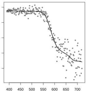
Since a larger distance before the reflection of the light is assumed to lead to less
received light, the relationship between range and logratio is modeled as a monotone decreasing spline function. Figure 7 shows the scatter plot for the data set and also
contains the estimated regression curve for the chosenλ.
●●●● ● ● ● ●●●●●●● ● ●● ● ● ● ● ●● ●● ●● ● ● ● ●● ●●● ●● ●● ●● ● ●●● ●● ● ● ● ●● ● ● ● ● ●●●● ● ● ● ● ● ● ● ● ● ● ●● ● ● ● ● ● ●●● ●● ● ●● ●● ● ●● ● ● ● ● ● ● ● ●● ● ● ● ● ● ● ● ● ● ● ● ● ● ● ● ● ● ● ● ●● ● ● ● ● ●● ● ● ● ●● ● ● ● ● ●● ● ●● ● ● ● ●● ● ● ● ● ● ● ● ● ● ● ● ● ● ● ● ● ● ● ● ● ● ● ● ● ● ● ● ● ● ● ● ● ● ● ● ● ●● ● ● ● ● ●● ●● ●● ● ● ●● ● ● ● ● ● ● ● ● ● ● ● ● ● ● ● ● ● ● ● ● ● ● ● ● 400 450 500 550 600 650 700 −0.8 −0.6 −0.4 −0.2 0.0 range logr atio
Figure 7: Scatter plot for the LIDAR data set with covariaterangeand dependent variablelogratio and fitted regression curve from the monotonicity restricted P-spline estimation with optimalλchosen with respect toGCV.
For this example, cubic splines are applied and the fitted regression curve is re-stricted to be monotone decreasing what is implemented via the constraint αj ≥ αj+1
m= 35 according to Equation (6). The smoothing parameterλis chosen with respect to
GCV(λ) =
Pn
i=1(yi−yˆi)2
(1−n1tr(H))2 (e.g. Ruppert et al., 2003, Section 5.3) with H=Hλ,constr being
the respective hat matrix as in Equation (10).
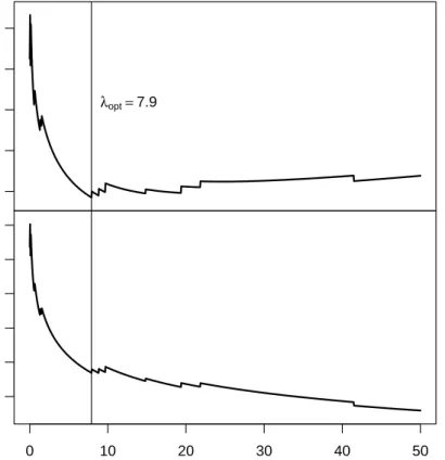
Figure 8 shows the GCV and tr(Hλ,constr) depending on λ. For λ = 7.9, GCV is
minimized and the corresponding tr(Hλ,constr) equals 9.4. Hence, for the given example
the degrees of freedom of the estimation are 9.4.
1.44 1.46 1.48 1.50 1.52 GCV λopt= 7.9 0 10 20 30 40 50 8 10 12 14 16 18 λ degrees of freedom
Figure 8: Smoothing parameterλvs.GCV (top) andλvs. degrees of freedom (bottom). Optimalλwith respect toGCV is 7.9 and corresponding degrees of freedom are 9.4.
At some values of λ, small jumps in the trace of the estimated hat matrix and hence also inGCV occur. This is due to the matrixCR in the hat matrix formula. Remember,
the matrix CR contains those rows of the constraint matrixC for whichCαˆ =0 holds.
With increasing λ, the penalty term forces the estimated regression curve to a straight
line and the monotonicity constraint becomes less important, hence the number of rows inCR decreases. Whenever the number of rows of CR changes, a little jump in Figure 8
5 Conclusion
A formula for calculating the hat matrix for an estimated regression model using a
mono-tonicity constrained and penalized spline is derived. The trace of this hat matrix can be interpreted as the equivalent to the degrees of freedom of the estimated model. It can be
used for example for model selection when criteria such as the Akaike information criterion or generalized cross validation are applied. In the context of penalized spline estimation,
it can be applied for the selection of the optimal smoothing parameter according to one of those criteria. For non-penalized as well as for penalized estimations, the order of the
spline, the number of knots and/or the position of the knots can, if not fixed in advance, be chosen analogously using the same selection criteria.
In an extensive Monte Carlo study, the hat matrices for six different DGPs and
R= 1000 samples are obtained. The results suggest that the degrees of freedom from the estimations fit the DGP functions appropriately. In an empirical example, the LIDAR
data set is analyzed and the degrees of freedom are found to be 9.4.
The presented hat matrix also works for the general case of an inequality constrained estimation with restriction Cβ ≥ 0. This general case includes semiparametric models
using monotonicity constrained splines for the nonparametric part of the model. In this case, the matricesD and Chave to be filled with zeros up to the appropriate dimension
and the remaining parts are just like in the case with only a single spline component.
Overall, this work helps practitioners to calculate the hat matrix of an estimated monotonicity constrained spline model and hence the degrees of freedom of an estimation,
what is an important task for example for model selection purposes including the search for an optimal smoothing parameter in the penalized case.
References
Bollaerts, K., Eilers, P. H. C., & Aerts, M. (2006). Quantile regression with monotonicity restrictions using P-splines and the L1-norm. Statistical Modelling, 6(3), 189–207.
de Boor, C. (2001). A Practical Guide to Splines, volume 27 of Applied Mathematical Sciences. Berlin: Springer, revised edition.
Dierckx, P. (1993). Curve and Surface Fitting with Splines. Numerical Mathematics and Scientific Computation. Oxford: Oxford University Press.
Eilers, P. H. C. & Marx, B. D. (1996). Flexible smoothing with B-splines and penalties.
Statistical Science, 11(2), 89–121.
Kagerer, K. (2013). A short introduction to splines in least squares regression analysis. University of Regensburg Working Papers in Business, Economics and Management
Information Systems 472, University of Regensburg, Department of Economics.
Paula, G. A. (1993). Assessing local influence in restricted regression-models.
Computa-tional Statistics & Data Analysis, 16(1), 63–79.
Paula, G. A. (1999). Leverage in inequality-constrained regression models. Journal of the
Royal Statistical Society: Series D (The Statistician), 48(4), 529–538.
R Core Team (2014). R: A Language and Environment for Statistical Computing. R
Foundation for Statistical Computing, Vienna, Austria.
Ruppert, D. (2002). Selecting the number of knots for penalized splines. Journal of
Computational and Graphical Statistics, 11(4), 735–757.
Ruppert, D. & Carroll, R. J. (2000). Spatially-adaptive penalties for spline fitting.
Aus-tralian & New Zealand Journal of Statistics, 42(2), 205–223.
Ruppert, D., Wand, M. P., & Carroll, R. J. (2003). Semiparametric regression, volume 12
of Cambridge Series in Statistical and Probabilistic Mathematics. Cambridge: Cam-bridge University Press.
Schumaker, L. L. (1981). Spline Functions Basic Theory. Pure and applied mathematics. John Wiley & Sons.
Wood, S. N. (2014). mgcv: Mixed GAM Computation Vehicle with GCV/AIC/REML smoothness estimation. R package version 1.7-29.