Data Descriptor:
A reconstruction
of global hydroclimate and
dynamical variables over the
Common Era
Nathan J. Steiger1, Jason E. Smerdon1, Edward R. Cook1& Benjamin I. Cook2
Hydroclimate extremes critically affect human and natural systems, but there remain many unanswered questions about their causes and how to interpret their dynamics in the past and in climate change projections. These uncertainties are due, in part, to the lack of long-term, spatially resolved hydroclimate reconstructions and information on the underlying physical drivers for many regions. Here we present the first global reconstructions of hydroclimate and associated climate dynamical variables over the past two thousand years. We use a data assimilation approach tailored to reconstruct hydroclimate that optimally combines2,978paleoclimate proxy-data time series with the physical constraints of an atmosphere—ocean climate model. The global reconstructions are annually or seasonally resolved and include two
spatiotemporal drought indices, near-surface air temperature, an index of North Atlantic variability, the location of the intertropical convergence zone, and monthly Niño indices. This database, called the Paleo Hydrodynamics Data Assimilation product (PHYDA), will provide a critical new platform for investigating the causes of past climate variability and extremes, while informing interpretations of future hydroclimate projections.
Design Type(s) data integration objective • source-based data transformation objective Measurement Type(s) hydroclimate
Technology Type(s) computational modeling technique Factor Type(s) proxy sensor
Sample Characteristic(s) Earth (Planet) • lake sediment • speleothem • glacial ice • borehole • marine sediment • coral reef • marine sponge reef • tree growth ring
1Lamont-Doherty Earth Observatory of Columbia University, Palisades, NY10964, USA.2NASA Goddard Institute for Space Studies, New York, NY10025, USA. Correspondence and requests for materials should be addressed to N.J.S. (email: [email protected]).
OPEN
Received:15February2018 Accepted:21March2018 Published:22May2018 1Background & Summary
Hydroclimate extremes, including persistent droughts and pluvials, can have extensive effects on societies and ecosystems. For example, multi-year droughts in California have caused significant agricultural losses, tree mortality, forestfires, and other impacts (e.g., refs 1–4). While the frequency of hydroclimate extremes are estimated to increase with global warming (e.g., refs 5–8), it is unclear if the underlying climate dynamics of such events are accurately produced in climate model simulations (e.g., refs 9–11) and if the models capture the full range of extremes on decadal and centennial time scales12,13. The lack of clarity on these issues is due in part to the lack of global reconstructions of droughts along with their associated dynamics. For example, the instrumental era lacks multidecadal ‘megadroughts’, known to have occurred throughout the past two millennia14,15. Hydroclimate reconstructions that include dynamical information therefore provide critical long-term perspectives and allow for better characterizations of the risks associated with future hydroclimate variability.
This work uses a data assimilation (DA) method to derive the first global reconstructions of hydroclimate and associated dynamical variables that span the last two millennia. In contrast to traditional reconstruction approaches and existing paleo-hydroclimate products, DA-based reconstruc-tion methods can simultaneously estimate both hydroclimatefields and corresponding atmosphere-ocean states16; having these two components is critical for analyses of the causes of hydroclimate extremes. DA for paleoclimate works by optimally fusing proxy information with the dynamical constraints of climate models17–21. Here we use proxy information from a network of 2,978 annually resolved proxy-data time series together with the Community Earth System Model Last Millennium Ensemble (CESM LME) of climate model simulations22. We perform three separate global reconstructions over the Common Era (the past 2000 years) at annual resolution (defined as April to the next calendar year March), the boreal growing season June through August (JJA), and the austral growing season December through February (DJF). We specifically reconstruct three global variables gridded at ~2 degree resolution: surface temperature at 2 m, the Palmer drought severity index (PDSI), and the standardized precipitation evapotranspiration index (SPEI). We also reconstruct the following climate indices at annual, JJA, and DJF temporal resolutions: the global mean temperature, the North Atlantic sea surface temperature index which is the non-detrended and non-smoothed version of the Atlantic multidecadal oscillation index (AMO), and the location of the intertropical convergence zone (ITCZ)23 in 11 longitudinal zones. Additionally we reconstruct the monthly Niño sea surface temperature (SST) indices (Niño 1+2, 3, 3.4, 4) and the monthly equatorial Pacific zonal SST gradient24. We reconstruct these specific climate index variables because they have been linked to hydroclimate variability and extremes across the globe. For example, Atlantic and tropical Pacific modes of variability have been linked to drought across North America (e.g, refs 25–32). Also, shifts in the ITCZ and consequent monsoonal changes over land have, for example, been associated with the collapse of the Maya Civilization33,34and the demise of the Angkor Empire35.
This Paleo Hydrodynamics Data Assimilation product (PHYDA), represents thefirst collection of global hydroclimate reconstructions along with their associated dynamical variables. It is also the first DA-based paleoclimate reconstruction to explicitly include the location of the ITCZ and monthly SST indices. We have also made several innovations in the reconstruction methodology compared to previous approaches19,20,36–38, including an algorithm that is more general and an order of magnitude faster, bias correction of the climate model variables, improved proxy system modeling, and a greatly expanded proxy network. Here we provide a thorough validation of all the reconstructed variables and also include a robust uncertainty estimation for all variables. These reconstructions can be used to more clearly elucidate the dynamics associated with droughts and pluvials on time scales ranging from seasons to centuries over the past two millennia: for example, they can be useful for assessing the causes of droughts in equatorial Africa or multidecadal droughts in the American West16. Additionally, the reconstructions are relevant for assessing model simulations and can be used to evaluate model projections of future hydroclimate variability and change (cf. refs 39,40).
Methods
Data assimilation
We employ a DA technique that optimally combines proxy data or observations with climate model states. The model provides an initial, or prior, state estimate that is updated based on the proxy observations and an estimate of the errors in both the observations and the prior. The general state update equations of DA41can be written as
xa¼xbþK½y-HðxbÞ; ð1Þ
where
K¼BHT½HBHTþR-1: ð2Þ
In these equations,xbis the prior (or‘background’) estimate of the state vector andxais the posterior (or ‘analysis’) state vector; the state vector contains all of the variables that are to be reconstructed. Observations (or proxies) are contained iny. The observations are estimated by the prior throughHðxbÞ,
which is, in general, a nonlinear vector-valued observation operator that mapsxbfrom the state space to the observation space. Bis the prior covariance matrix,R is the error covariance matrix for the proxy
data, and H represents a linearization of H. In a general sense, the reconstruction process works by computing an optimal linearfit between the initial guess of the climate state, the priorxb, and the proxies
y. Because proxies are available at annual time steps, a reconstruction is made by iteratively computing equations (1) and (2) for each year (or season within each year) of the existing proxy data.
We implement the general DA equations described above by using an ensemble square rootfilter from ref. 42. Though the authors of ref. 42 recommend the sequential assimilation of observations for computational reasons, the simultaneous assimilation of observations is actually an order of magnitude faster in contemporary matrix-optimized computing software, such as MATLAB. We therefore modified previous approaches used for paleoclimate DA19,20,36–38 and specifically implemented the matrix equations from ref. 42, as listed below in equations (3)-(9). These equations begin with the prior ensemble state estimatexb, which is anm×nmatrix wheremis the state size (e.g., if only temperaturefields are
reconstructed then mwill be the number of grid points in the spatial temperature field) and nis the ensemble size. The prior is then separated into anm× 1 ensemble meanxband them×ndeviations from
this meanx0b(the mean is removed from each row ofxb). The implementation subsequently updates the ensemble mean and the deviations from the ensemble mean separately:
xa¼xbþK½y-HðxbÞ; ð3Þ xa0 ¼x0b-KH~ ðx0bÞ; ð4Þ
where the parantheses inHðxbÞandHðxb0Þdenote the operatorHacting onxbandx0b. The observation
vector yis of dimension p× 1, where pis the number of proxy data values available in a given time interval (e.g., a year or season) andHðxbÞandHðx0bÞhave respective dimensions ofp× 1 andp×n. The
two Kalman gain matrices are calculated as
K¼BHT½HBHTþR-1; ð5Þ and ~ K¼BHT hpffiffiffiffiffiffiffiffiffiffiffiffiffiffiffiffiffiffiffiffiffiffiHBHTþRi-1 T ffiffiffiffiffiffiffiffiffiffiffiffiffiffiffiffiffiffiffiffiffiffi HBHTþR p þpffiffiffiffiR h i-1 ; ð6Þ
whereRis thep×pobservational-error covariance matrix, square roots indicate a matrix square root,−1 superscripts indicate a matrix inverse, T superscripts indicate a matrix transpose and where
BHT¼ 1 n-1x 0 b½Hðx0bÞT; ð7Þ and HBHT¼ 1 n-1Hðx 0 bÞ½Hðx0bÞT: ð8Þ
After computing equations (3)-(8) the full posterior ensemble is then recovered through
xa¼xaþx0a; ð9Þ
wherexais added to each column ofx0a. Collectively, equations (3)-(9) are computed for each year (or a
particular season of each year) to arrive at a series of posterior ensemble state estimates that together constitute the probabilistic spatiotemporal reconstruction. In the reconstruction files for all variables (Data Citation 1) we have included the posterior ensemble mean, 1 standard deviation of the posterior ensemble as well as its 5th, 50th, and 95th percentiles; this error estimate explicitly includes uncertainty information from the spread in the climate model prior (HBHT) as well as the error in the proxy models (R).
In our implementation of equations (3)-(9), R is assumed to be a diagonal covariance matrix (uncorrelated errors) where the entries are the error variance of each proxy (defined in the‘Proxy system models’section). If the proxy errors are correlated then equations (3)-(9) can be computed in the same way using a non-diagonalR.
Climate model data and reconstruction variables
As in previous studies19,20,36–38we use an offline DA approach in whichxbis the same for each year and is drawn from an existing climate model simulation: the ensemble members are seasonally or annually-averaged climate states instead of an ensemble of independently running model simulations, as in traditional online DA. This approach therefore propogates no information forward in time (e.g.,xafrom
year t−1 is not used as xb in year t) and only the proxies constrain the time evolution of the reconstruction. In principle, the ensemble members can be drawn from a single long simulation, multiple simulations or even from simulations of a collection of climate models; to be informative for the reconstruction, the prior should be representative of what one is trying to reconstruct (e.g., to reconstruct a year with a large volcanic eruption, the prior should include ensemble members that contain such events). According to many previous reconstruction experiments19,20,36–38,43 year-specific forcing or boundary condition information appears to be unnecessary for skillful reconstructions as long as the 3
prior is sufficiently representative. Furthermore, the offline approach can be performed without the immense computational costs of a traditional online approach.
We construct the priorxbusing the CESM LME22, which used atmosphere and land components with ~2-degree resolution and ocean and sea ice components with ~ 1-degree resolution. The simulations were run from the years 850 to 1850 CE using estimates of the transient evolution of solar intensity, volcanic emissions, greenhouse gases, aerosols, land-use conditions, and orbital parameters44. The simulations were given identical forcings but differed by round-off error in the initial atmospheric state; this difference was sufficient to generate simulations with different internal ocean-atmosphere variability and therefore different time histories (e.g., annual Niño 3.4 indices from the simulations are uncorrelated). For the reconstruction prior, we used a single simulation, number 10 from the full-forcing ensemble, to generate our prior ensemble; specifically, we used the middle 998 years of the CESM simulation excluding the two simulation endpoints to create a static 998 member prior ensemble that was used to estimate the climate state in each year of the reconstruction (the last year cannot be used because of the particular annual averaging we used here and thefirst year cannot be used because the variable SPEI integrates the previous 12 months of climate information, therefore only the second year of an SPEI time series is meaningful). This prior is consistent with previous work that has established that the prior is not required to contain year-specific forcing or boundary condition information, rather it must merely be statistically representative of the reconstruction period19,20,36–38,43. Here and in theoretical tests of the methodology38 we performed sensitivity tests with different members from the CESM LME and found no discernible differences in the results. Previous work has shown that the choice of climate model prior has little impact on the DA reconstructions when the choice is among the publicly available millennial-length coupled simulations20. However, model biases in the temperature and precipitation fields are specific to each model and can influence the fidelity of the reconstructions. To partially account for issues related to biases, we bias-corrected the climate model temperature and precipitation fields by replacing their monthly mean climatologies with observational monthly mean climatologies from refs 45,46.
Reconstructions were performed from the years 1–2000 CE targeting three different temporal windows: annual means (defined as April to the next calendar year March), the boreal growing season of JJA, and the austral growing season of DJF. The particular annual average used herein was chosen to account for the seasonal cycle of a global network of proxies as well as climate phenomena like the El Niño—Southern Oscillation, the continuity of which would be ignored with a calendar year average. Except for the monthly Niño SST indices described below, all other variables were reconstructed over the annual, JJA, or DJF windows.
Each reconstruction contains the following griddedfields over the global domain: 2 m air temperature, PDSI, and SPEI using a 12-month decaying exponential weighting kernel47chosen to closely resemble the time scale of PDSI; the potential for skillful reconstruction of these fields was previously demonstrated using pseudoproxy experiments16. Both PDSI and SPEI were computed using the Penman-Monteith equation for potential evapotranspiration and monthly climate model output of precipitation, 2 m temperature, vapor pressure, net surface radiation, surface pressure, and surface wind (estimated from 10 m down to 2 m using the wind profile power law); the climatologically bias-corrected temperature and precipitation fields were used in the calculations. PDSI was computed using the MATLAB code from ref. 48, which produces the standard formulation of PDSI as opposed to self-calibrating versions (e.g., ref. 49). Both PDSI and SPEI are broadly used in drought monitoring50 and historical drought reconstructions14,15,51–54.
We also reconstruct the following index variables: the area-weighted global mean temperature, the North Atlantic SST index which is the non-detrended and non-smoothed version of the Atlantic multidecadal oscillation (AMO), the monthly Niño SST indices (Niño 1+2, 3, 3.4, 4), the monthly equatorial Pacific zonal SST gradient24, and the location of the intertropical convergence zone (ITCZ) in 11 longitudinal zones. Because there are different smoothing and standardization conventions in computing Niño SST indices, we have simply computed the area-averaged monthly SST values in each Niño region. We use the definition of the location of the ITCZ from23, which is the expected value of precipitation (P) using a 10th-power area weighting, integrated over the tropical latitudesϕ1andϕ2,
ϕITCZ¼ Rϕ2 ϕ1 ϕ½cosð ÞϕP 10dϕ Rϕ2 ϕ1 ½cosð ÞϕP 10dϕ ð10Þ
In equation (10), we use the annual or seasonally averaged precipitation and alsoϕ1=30°S andϕ2=30°N to account for Monsoon regions where the seasonal precipitation maximum can extend far beyond the equator. Following refs. 23,55 we interpolate the tropical precipitation to a 0.1 degree latitudinal grid before computing equation (10). The 11 longitudinal zones are listed in the tables and include all major ocean and land regions in the tropics (e.g., continental Africa and the Atlantic) and for different definitions of these regions (e.g., different definitions of the Pacific ITCZ sector). Note that for computation simplicity, all of the reconstructed index variables are included in the prior state vector rather than being post-processed from reconstructed spatial climate fields. The monthly indices are reconstructed by the appended state method where here for example, each monthly index occupies 12 elements in the state vector of a given ensemble member.
Proxy data
Two proxy databases form the foundation of the database: the updated PAGES2k database56and the tree-ring width collection of ref. 57. Additionally, 59 publicly available proxy records including ice cores, speleothems, and lake sediments were also included. In total this database includes 2,978 annually resolved proxies after removing duplicates; only annually or seasonally resolved proxy data values are used such that we include only the annually resolved portions of mixed-resolution proxies. This constitutes the largest multiproxy database employed thus far in a global reconstruction. Figure 1 shows the spatial and temporal distribution of the combined proxy network, with the numbers of each proxy type indicated in the caption. Note that the ice core, speleothem, and sediment records have been grouped together because they are modeled similarly in the proxy system modeling framework (see the following section). Age model uncertainties for the relevant proxy types are only accounted for through our use of the best estimate of the annual ages as determined by the authors of each proxy dataset. The full proxy database and additional proxy metadata is publicly available (Data Citation 2).
Proxy system models
DA-based reconstructions must use climate model variables to estimate proxy observations (HðxbÞ in
Equation 1). For example, a given climate model's temperature and precipitation can be used to estimate tree-ring width through a sub-model. Such‘forward models’are referred to in paleoclimatology as proxy system models (PSMs)58. Here we employ statistical, regression-based PSMs that are specific to each proxy; this improves on previous DA-based reconstructions that used only a univariate linear regression with temperature for all proxies20. Wefirst illustrate this procedure for the‘other records’in Fig. 1. The PSMs for these proxies are derived from linear regressions between theithannual proxy time series,pi,
and the local instrumental temperature series from ref. 45 indicated byXi. Eachpiis standardized to unit
Year 0 500 1000 1500 2000 Number of proxies 0 500 1000 1500 2000 2500 3000 Tree-ring records Coral records Other records
Tree-ring records Coral records Other records
Tree-ring records Coral records Other records
a
b
Figure 1. Proxy data network and temporal availability. (a)Spatial distribution of the combined proxy data network from refs. 56 and 57. Proxies are categorized by how they are modeled in the proxy system modeling framework: 2591 tree rings, 197 corals and sclerosponges, and 190 other records, which include 153 ice core isotope records, 26 speleothem isotope records, 10 lake sediment records, and 1 marine sediment record.(b) Temporal availability of the proxy network by proxy type.
variance and for the three different reconstructions discussed previously,Xiis either an annual, JJA, or
DJF average. The regression equation is
pi¼αiþβiXiþεi; ð11Þ
which is calculated over the available temporal overlap between the proxy and the instrumental time series within the calibration period 1920–2000 (leaving approximately 5 decades for a verification interval of 1871–1919, consistent with many previous studies, e.g., refs 59–61). We chose to throw out all proxies that did not have at least 20 overlapping values for the regression (for all proxy types this amounted to a total of 82 proxies that were not used because they did not extend sufficiently through the calibration interval). The prior estimate of the proxies,HðxbÞi, is then found for each proxy by using the calibrated
parametersαiandβiin
HðxbÞi¼αiþβiXi; ð12Þ
whereXiare the corresponding climate model temperature grid point values nearest to the proxy location
in each prior ensemble member. The vector of residuals for each proxy,εi, are then used to compute the
diagonal entries of the matrix R, where the ith entry is computed as Ri¼ε2i. Note that this statistical
model only considers local information and relies solely on the Kalman gain covariance relationships to inform non-local climate variables. We did not employ a physically-based PSM for the oxygen isotope proxies, such as for ice-core δ18O, because of the lack of available high resolution millennial-length simulations with water istopes and because previous work has indicated no improved reconstruction performance using such PSMs over a linear regression with local temperature38.
The PSM for tree rings is modeled similar to the approach above but with either local instrumental temperature or local instrumentally-derived PDSI62, depending on which instrumental data type has the highest absolute correlation with the proxy over the calibration period. This correlation is computed using the averaging time scale of the reconstruction such that it is possible for a given site to be modeled with temperature for one time average and PDSI for another time average. For the annual reconstruction, 1719 tree-ring chronologies were modeled with PDSI while 872 were modeled with temperature; for the
JJA DJF Apr-Mar
T2m
SPEI
PDSI SPEI T2m PDSI SPEI T2m
Skill -0.4 -0.2 0 0.2 0.4 0.6 0.8
PDSI SPEI T2m PDSI SPEI T2m
Skill -0.4 -0.2 0 0.2 0.4 0.6 0.8
PDSI SPEI T2m PDSI SPEI T2m
Skill -0.4 -0.2 0 0.2 0.4 0.6 0.8 CRPSS r r CRPSS r CRPSS
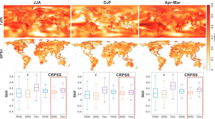
Figure 2. Skill assessments for the temperature and hydroclimate reconstruction products computed over the years 1901–2000.Thetop rowshows the mean continuous ranked probability skill score (CRPSS) for the 2 m temperature reconstruction (T2m). CRPSS is computed for each grid point time series with the observational temperature dataset of Berkeley Earth45. Themiddle rowshows the CRPSS for the standardized precipitation-evapotranspiration index (SPEI). The observational SPEI is computed with a 12-month decaying exponential kernel and using the CRU TS3.23 land surface datasets69. Thebottom rowsummarizes the spatial skill values from the top two rows (orange and purple CRPSS box plots contained within the red boxes) as well as corresponding CRPSS assessments for the Palmer drought severity index (PDSI) and also correlation (r) skill values over the same time period. For the PDSI assessments, we use the observational product of ref. 62.
JJA reconstruction 1579 were modeled with PDSI and 1012 with temperature; and for the DJF reconstruction 1572 were modeled with PDSI and 1019 with temperature. Using both temperature and PDSI in the PSMs is necessary because of the heterogenous sensitivities of different tree-ring sites and the inclusion of both tree ring-width and density; additionally, using both temperature and moisture sensitive trees is essential for producing a skillful DA-based reconstruction of both temperature and moisture
fields16.
We employ a bivariate regression-based PSM based on ref. 63 for the coral and sclerospongeδ18O proxies. This PSM uses both SST and sea surface salinity to estimate proxy δ18O. Here we calculate regression parameters for each site individually using the long-term ocean reanalysis from ref. 64 instead of basin or region-wide parameter values as used in ref. 63. For non-δ18O coral proxies, we employ a linear univariate regression with SST.
Code availability
The MATLAB code (https://www.mathworks.com/products/matlab.html) necessary to perform the reconstructions discussed in this data descriptor are available athttps://github. com/njsteiger/PHYDA under a free BSD license. The reconstructions were performed using MATLAB version R2015a.
Data Records
Each of the three reconstructions constituting thefirst version of PHYDA are publicly available at the Zenodo data repository as NetCDF4 files (Data Citation 1), which include all of the reconstructed variables and their uncertainties; specifically this includes the posterior ensemble mean, 1 standard deviation of the posterior ensemble as well as its 5th, 50th, and 95th percentiles. The NetCDF4 format also incorporates all of the associated variable metadata. The paleoclimate proxy database used herein is also publicly available at the Zenodo data repository (Data Citation 2).
Technical Validation
We validate the reconstructions against observations primarily using two skill metrics: Pearsons' correlation (r) and the mean continuous ranked probability skill score (CRPSS). Correlation is computed using only the reconstruction mean time series at each grid point while the CRPSS metric accounts for both the mean grid point time series as well as the grid point uncertainty estimates. CRPSS is based on the continuous ranked probability score (CRPS), which is a‘strictly proper’scoring rule that accounts for the skill of the entire posterior reconstruction distribution65. CRPS penalizes bias, incorrect variance, incorrect phasing, and an ensemble spread that is either too wide or overconfident. Because the posterior
Variable r (1871–2000) CRPSS (1871–2000) r (1871–1919) CRPSS (1871–1919) GMT 0.88 0.56 0.35 0.41 AMO 0.71 0.33 0.48 0.53 Nino 1+2 0.18 -0.12 0.18 −0.10 Nino 3 0.45 0.24 0.42 0.28 Nino 3.4 0.60 0.41 0.55 0.45 Nino 4 0.59 0.44 0.37 0.37 ΔSST Pacific 0.10 -0.01 0.11 0.04
coh 2.5 yr (1871–2000) coh 5 yr (1871–2000) coh 10 yr (1871–2000) CE (1871–1919)
GMT 0.42 0.53 0.74 0.77 AMO 0.40 0.38 0.61 0.39 Nino 1+2 0.70 0.81 0.56 −2.69 Nino 3 0.83 0.87 0.70 −1.11 Nino 3.4 0.86 0.90 0.79 −0.16 Nino 4 0.87 0.87 0.74 −0.17 ΔSST Pacific 0.17 0.67 0.45 −2.88
Table 1. Verification of annual mean index variables and monthly SST variables.Verifications include the area-weighted global mean temperature (GMT), the North Atlantic SST index which is the non-detrended and non-smoothed version of the Atlantic multidecadal oscillation (AMO), the monthly Niño SST indices (Niño 1+2, 3, 3.4, 4), and the monthly equatorial Pacific zonal SST gradient (ΔSST Pacific). Skill metrics include correlation (r), mean continuous ranked probability skill score (CRPSS), coherence at the specific periods of 2.5, 5, and 10 years, and the coefficient of efficiency (CE). Each metric includes the period over which it was computed except for CE where the years indicate the verification mean time period.
ensemble estimates are approximately normally distributed we use equation (5) from ref. 66, crps¼σ yn2ΦðynÞ-1þ2ϕ yn - 1ffiffiffi π p ; ð13Þ
whereyn=(y−μ)/σ, withybeing the observed value,μthe mean of the posterior ensemble estimate, and σ the standard deviation of the posterior ensemble, and where ϕ(yn) and Φ(yn) are respectively the
normal probability density function and the normal cumulative distribution function ofyn. Note that this
implementation assumes that there is no error in the observations. All of our uses of equation (13) are for time series, either individual time series or grid point time series. We therefore compute the mean of all the time-step values of equation (13) and denote it as CRPS. The skill score version, CRPSS, is the reconstructed CRPS computed with respect to the CRPS of a reference distribution, CRPSS≡1−CRPSrec/ CRPSref, here the initial uninformed prior. We use CRPSS instead of CRPS because CRPS has the referenceless range of [0,∞) while CRPSS has the range (−∞, 1] with positive CRPSS indicating that the reconstructed distribution is more skillful for this metric than the uninformed prior. CRPSS is generally a more stringent skill metric than correlation, so we focus here primarily on CRPSS. Additionally, for
Variable r (1871–2000) CRPSS (1871–2000) r (1871–1919) CRPSS (1871–1919) GMT 0.87 0.60 0.51 0.42 AMO 0.72 0.42 0.47 0.42 Nino 1+2 0.19 −0.10 0.22 −0.06 Nino 3 0.45 0.20 0.48 0.24 Nino 3.4 0.56 0.32 0.56 0.29 Nino 4 0.50 0.31 0.39 0.19 ΔSST Pacific 0.07 0.01 0.06 0.07
coh 2.5 yr (1871–2000) coh 5 yr (1871–2000) coh 10 yr (1871–2000) CE (1871–1919)
GMT 0.56 0.59 0.70 0.80 AMO 0.38 0.48 0.53 0.49 Nino 1+2 0.69 0.83 0.46 −2.65 Nino 3 0.81 0.88 0.63 −1.32 Nino 3.4 0.85 0.91 0.71 −0.55 Nino 4 0.87 0.86 0.62 −0.79 ΔSST Pacific 0.13 0.41 0.29 −2.85
Table 2. Verification of JJA mean index variables (GMT and AMO) and monthly SST variables (Niño 1+2, 3, 3.4, 4 andΔSST Pacific), cf. Table 1.
Variable r (1871–2000) CRPSS (1871–2000) r (1871–1919) CRPSS (1871–1919) GMT 0.79 0.34 0.20 0.33 AMO 0.55 0.13 0.09 0.28 Nino 1+2 0.19 −0.19 0.18 −0.21 Nino 3 0.44 0.10 0.40 0.15 Nino 3.4 0.55 0.23 0.51 0.34 Nino 4 0.59 0.27 0.44 0.37 ΔSST Pacific 0.10 −0.06 0.13 −0.06
coh 2.5 yr (1871–2000) coh 5 yr (1871–2000) coh 10 yr (1871–2000) CE (1871–1919)
GMT 0.58 0.41 0.66 0.42 AMO 0.17 0.52 0.37 −0.11 Nino 1+2 0.60 0.78 0.58 −3.09 Nino 3 0.75 0.88 0.78 −1.89 Nino 3.4 0.75 0.88 0.87 −0.93 Nino 4 0.79 0.87 0.82 −0.92 ΔSST Pacific 0.31 0.77 0.54 −3.19
Table 3. Verification of DJF mean index variables (GMT and AMO) and monthly SST variables (Niño 1+2, 3, 3.4, 4 andΔSST Pacific), cf. Table 1.
validating the time series reconstructions we use the metrics of the coefficient of efficiency67 and the cross-spectral coherence computed using a multi-taper method68.
The top two rows of Fig. 2 show the skill of the reconstructed 2 m temperature and SPEI at each grid point using the CRPSS skill metric. The bottom row of Fig. 2 summarizes the spatial skill in box plots for all the spatial variables using r in addition to CRPSS. Seasonal (JJA and DJF) and annual reconstructions are organized by column. The skill metrics are computed for the years 1901–2000 against Berkeley Earth45 for temperature and an observational SPEI computed with a 12-month decaying exponential kernel and using the CRU TS3.23 land surface datasets69; the interval of 1901–2000 is chosen because CRU TS3.23 only extends back to the year 1901. The skill assessments do not include Antarctica because of the sparsity of observational data in this region and because hydroclimate indices are not suited for use over ice-covered landscapes. Assessments of PDSI are included in the bottom row of Fig. 2. We note that the reconstruction uses standard PDSI while the observational verification data62 uses the slightly different self-calibrating version of PDSI.
It is important to note that in Fig. 2 we compute the skill metrics over the interval 1901–2000 while the parameters of the PSMs are fit to observations over the interval of 1920–2000. In traditional reconstruction techniques (e.g., ref. 70) it would not be suitable to show validation statistics over the calibration interval because the instrumental data are used to bothfit the proxy data and also for the reconstruction target. In contrast, the PSM parameterfitting here is not an equivalent process because the target field is a pre-industrial climate model simulation and the temporal information is only derived from the proxies. However, in validating these reconstructions we do not rely solely on skill metrics computed over a significant fraction of the PSM calibration interval. In Tables 1–3 we additionally compute skill metrics for the temperature-based climate indices over the period 1871–1919.
Skill tends to be highest in the tropics and nearby the proxy locations (cf. Fig. 1) during the summer growing season, as is evident, for instance when comparing JJA and DJF reconstruction skill over North America. The annual results also compare favorably with the seasonal reconstructions, particularly over the tropics, showing that it is possible to provide skillful results across a range of time intervals using this DA approach, thus verifying the theoretical results of previous pseudoproxy experiments16. The box plots in the bottom row of Fig. 2 show generally consistent results across the seasons and variables, though the temperature reconstructions are generally more skillful than the PDSI or SPEI reconstructions, while
Tree-ring records Coral records Other records
MADA
ANZDA OWDA
NADA
MXDA
Figure 3. Reconstruction assessment using drought atlases.Correlation between the data assimilation-based PDSI reconstruction and the PDSI reconstructions of the drought atlases from the years 1500–2000: the North American drought atlas (NADA)14,51, the Old World drought atlas (OWDA)15, the Monsoon Asia drought atlas (MADA)52, the Mexican drought atlas (MXDA)53, and the Australia and New Zealand drought atlas
(ANZDA)54. Correlations are computed using the JJA reconstruction for NADA, OWDA, MADA, and MXDA and the DJF reconstruction for ANZDA. Prior to computing the correlations, the drought atlases were interpolated to the land surface grid of the CESM LME model simulation used in the data assimilation-based reconstruction presented here.
PDSI and SPEI are fairly comparable. Though not shown, the spatial patterns of r are similar to those of CRPSS: for example, the JJA SPEI spatial correlation between the r and CRPSS maps is 0.70 while the corresponding spatial correlation between r and CRPSS for JJA 2 m temperature is 0.68. However, unlike CRPSS, r is consistently high across regions that possess many proxies; this can be seen, for example, when contrasting the CRPSS metric of JJA SPEI (Fig. 2) with r of JJA PDSI in northern Mexico (Fig. 3). As further validation, we also compare the PDSI reconstructions to the available Drought Atlases14,15,51–54(Fig. 3). Each of the drought atlases have been extensively validated and represent the current gold-standard PDSI reconstruction product. The correlations in Fig. 3 cover the period 1500–2000 and indicate a DA reconstruction that is strongly consistent with the drought atlas products, particularly over North America and Europe where in some locales correlations approach 1; similarly high correlations exist for 100 year intervals through time as well as for the entire length of each drought atlas (which have heterogeneous start times). The agreement between the reconstructions and the drought atlases is remarkable given the vastly different methods used to derive the PDSIfields and that the proxy datasets were not designed to contain the same inputs nor use the same proxy data processing methods (though there is some overlap between the proxy network used herein and the proxy networks of the drought atlases). However, we note a more muted agreement for the ANZDA and also in regions where the proxy network used in the DA reconstruction has limited or no data; where there is little or no data, the prior ensemble often cannot be sufficiently constrained, resulting in localized regions of low Figure 4. Reconstruction verification for three representative climate-dynamical indices. (a)Verification of the annual mean North Atlantic sea surface temperature index (NASST), which is the detrended, non-smoothed version of the Atlantic multidecadal oscilation (AMO). This panel includes the AMO observations (Obs.)76and the mean reconstruction (Recon.) with a corresponding±2σrange of the posterior ensemble. Skill
values are indicated for correlation (r) and the mean continuous ranked probability skill score (CRPSS) in the bottom left corner. These skill values are computed over the entire time interval shown.(b)Reconstruction verification of the location of the annual mean intertropical convergence zone (ITCZ) over the South Asian monsoon region spanning the tropics from 65°E to 95°E. The observational ITCZ is computed using the Global Precipitation Climatology Project version 2.3 (ref. 46) available back to the year 1979. Skill values of r and CRPSS are computed over the time interval shown here.(c)Reconstruction verfication for the monthly Niño 3.4 index, similar to (a) and (b). The observational Niño 3.4 index is computed from Berekley Earth surface temperature dataset45, which over the ocean is based on HadSST77.(d)Coherence as a function of frequency and period between the mean Niño 3.4 reconstruction and the observations shown in panel (c).
skill16,19,38. The two skill metrics presented in both Fig. 3 and Fig. 2 provide complimentary measures for establishing the skill of the spatialfield reconstructions.
The reconstructed dynamical climate indices span the globe and include many drivers of hydroclimate variability. Figure 4 shows representative verifications of three of these indices: (a) the AMO, (b) the location of the ITCZ over the South Asian monsoon region, and (c) the monthly Niño 3.4 index, with Fig. 4(d) showing the cross-spectral coherence of the reconstructed and observation-based Niño 3.4 index. The panels in Fig. 4 illustrate that a range of important climate indices from different regions are skillfully reconstructed, with high positive correlations, CRPSS, and coherence values. We highlight in particular that these are thefirst DA-based paleoclimate reconstructions of the location of the ITCZ and monthly Niño indices.
We have additionally performed an exhaustive verification of all the reconstructed index variables. Tables 1–3 present several skill metrics for each of the temperature-based variables: r and CRPSS over the interval 1871–2000, r and CRPSS over the interval 1871–1919, cross-spectral coherence at the specific periods of 2.5, 5, and 10 years (as in Fig. 4 where the full range of coherence is shown), and CE using the verification mean of 1871–1919 (mimicking a traditional calibration—validation skill test, where here the calibration period is the period over which the PSMs were trained). We note, however, that unlike CRPSS, CE is not a strictly proper scoring metric for ensemble reconstructions65; we also note that both r and CRPSS do not incorporate two time periods as in CE, so r (or r2) is not directly comparable with CE in the manner traditionally used in statistical dendroclimatology71. These skill values are all shown for the annual (Table 1), JJA (Table 2), and DJF (Table 3) reconstructions. Many variables show skill (positive values) across many or all metrics with some variables having particularly high values, such as global mean temperature (GMT) with r=0.88, CRPSS=0.56, and CE=0.77 (Table 1). A few variables, such as the monthly Niño 1+2 index, appear to have skill only at multiyear time scales, low r and negative CRPSS and CE yet high coherence at 2.5, 5, and 10 year periods (Table 1). We note that the negative CE values for the monthly Niño indices (Tables 1,2,3) are the result of an annual cycle that shows up too strongly in
Region Longitudinal range (deg E) r (1979–2000) CRPSS (1979–2000)
Tropical East Africa [28, 50] 0.59 0.32
Indian Ocean [50, 95] 0.71 0.52
South Asia [65, 95] 0.78 0.57
Indonesia [95, 130] 0.72 0.33
East Pacific Ocean [130, 170] −0.01 0.13
Pacific Ocean [130, 260] 0.77 0.41
Pacific Ocean [160, 260] 0.80 0.37
West Pacific Ocean [170, 260] 0.83 0.36
Tropical South America [260, 320] 0.19 0.16
Atlantic Ocean [320, 345] 0.35 0.35
Tropical Africa [345, 50] −0.05 0.26
Table 4. Verification of the ITCZ variables at annual resolution.Regions are named and given the longitudinal ranges that they cover (in degrees eastward from the Prime Meridian, in keeping with the convention of climate model grids.) Each metric includes the period over which it was computed.
Region Longitudinal range (deg E) r (1979–2000) CRPSS (1979–2000)
Tropical East Africa [28, 50] −0.04 0.30
Indian Ocean [50, 95] 0.64 0.52
South Asia [65, 95] 0.36 0.31
Indonesia [95, 130] 0.41 0.33
East Pacific Ocean [130, 170] 0.05 0.15
Pacific Ocean [130, 260] 0.71 0.48
Pacific Ocean [160, 260] 0.73 0.49
West Pacific Ocean [170, 260] 0.75 0.49
Tropical South America [260, 320] 0.29 0.27
Atlantic Ocean [320, 345] −0.08 0.27
Tropical Africa [345, 50] −0.33 0.22
Table 5. Verification of the ITCZ variables at JJA mean resolution, cf. Table 4.
the reconstructions; r does not account for variance, coherence is looking at multiyear time scales where there is not a variance issue, and CRPSS considers several factors in the reconstruction that outweigh too much variance in this instance. At an annual average of the indices, when the annual cycle is averaged out, all CE values improve; for the reconstruction using annual PSMs and using the tropical annual average defined previously, Niño 1+2 CE=0.37, Niño 3 CE=0.34, Niño 3.4 CE=0.35, Niño 4 CE=0.07, and ΔSST Pacific CE=0.12 (cf. the corresponding column in Table 1). Tables 4,5,6 show the r and CRPSS metrics for all of the ITCZ reconstructions, which are limited to the period of 1979–2000 because the Global Precipitation Climatology Project version 2.3 (ref. 46) is only available back to the year 1979. All of the ITCZ reconstructions are skillful in at least one season, though the skill in some regions is strongly dependent on the season, e.g., the Tropical East Africa annual mean versus JJA and DJF (top row in Tables 4–6).
The series of validation tests presented in this section include 2 measures of spatial skill, r and CRPSS, 18 box plots summarizing the spatial skill of all spatially-resolved variables, and 6 tables with a total of 168 entries verifying the skill of the reconstructed climate indices. These assessments have been done with different skill metrics over three different time intervals (both observational and paleo time intervals) to ensure that a robust picture of each variable's skill can be seen. These validation tests show that many variables are skillfully reconstructed but the level of skill is dependent on the region, the variable, the season (e.g., JJA versus DJF), and the timescale (e.g., annual versus decadal). Future versions of PHYDA will include high-resolution climate model simulations for the prior from the upcoming Paleoclimate Model Intercomparison Project phase 4 (ref. 72), including a more sophisticated bias-correction scheme (e.g., refs 73,74), updates to the proxy network (such as the inclusion of all the tree-ring records used in the drought atlases), and updates to the PSMs as they become further developed.
Usage Notes
Paleoclimate reconstructions rely on a relatively sparse network of noisy proxy data time series and the reconstruction may have significant uncertainty depending on the variable, the location, and the time period of interest75. Before using PHYDA for analyses, users should consult the relevant spatial verification Figs. 2,3 or Tables (1–6) to determine whether the variables of interest can provide useful information. It is also important to consider the range of uncertainty on the variable of interest (included in the NetCDF4 files) and not just the ensemble mean. Because of the decreasing proxy availability further back in time (Figure 1b) the uncertainty in the reconstruction correspondingly increases. Because of how the DA reconstruction methodology is formulated, decreasing amounts of information from proxies will yield a corresponding decrease in the variance of the ensemble mean reconstruction as the prior becomes more heavily relied upon; this gradual reduction in variance of the ensemble mean should not be interpreted as a reduction in the variance of the historical climate.
References
1. Howitt, R., Medelln-Azuara, J., MacEwan, D., Lund, J. R. & Sumner, D.Economic analysis of the 2014 drought for California agriculture(Center for Watershed Sciences University of California: Davis, CA, 2014).
2. Asner, G. P.et al.Progressive forest canopy water loss during the 2012-2015 California drought.Proc. Natl. Acad. Sci. USA113, E249–E255 (2016).
3. Abatzoglou, J. T. & Williams, A. P. Impact of anthropogenic climate change on wildfire across western us forests.Proc. Natl. Acad. Sci. USA113,11770–11775 (2016).
4. Young, D. J. N.et al.Long-term climate and competition explain forest mortality patterns under extreme drought.Ecol. Lett.20, 78–86 (2017).
5. Battisti, D. S. & Naylor, R. L. Historical warnings of future food insecurity with unprecedented seasonal heat.Science323, 240–244 (2009).
Region Longitudinal range (deg E) r (1979–2000) CRPSS (1979–2000)
Tropical East Africa [28, 50] 0.04 0.27
Indian Ocean [50, 95] 0.33 −0.13
South Asia [65, 95] 0.32 −0.01
Indonesia [95, 130] 0.40 0.27
East Pacific Ocean [130, 170] 0.20 0.12
Pacific Ocean [130, 260] 0.32 0.32
Pacific Ocean [160, 260] 0.34 0.27
West Pacific Ocean [170, 260] 0.40 0.28
Tropical South America [260, 320] 0.57 0.34
Atlantic Ocean [320, 345] −0.09 0.10
Tropical Africa [345, 50] 0.33 0.04
6. Kirtman, B.et al.Near-term climate change: Projections and predictability. InClimate Change 2013: The Physical Science Basis. Contribution of Working Group I to the Fifth Assessment Report of the Intergovernmental Panel on Climate Change(Cambridge Univ. Press, Cambridge, UK, 2013).
7. Cook, B. I., Ault, T. R. & Smerdon, J. E. Unprecedented 21st century drought risk in the american southwest and central plains. Sci. Adv1,1–7 (2015).
8. Diffenbaugh, N. S., Swain, D. L. & Touma, D. Anthropogenic warming has increased drought risk in California.Proc. Natl. Acad. Sci. U.S.A.112,3931–3936 (2015).
9. Aloysius, N. R., Sheffield, J., Saiers, J. E., Li, H. & Wood, E. F. Evaluation of historical and future simulations of precipitation and temperature in central Africa from CMIP5 climate models.J. Geophys. Res. Atmos121,130–152 (2016).
10. Swann, A. L. S., Hoffman, F. M., Koven, C. D. & Randerson, J. T. Plant responses to increasing CO2 reduce estimates of climate impacts on drought severity.Proc. Natl. Acad. Sci. USA113,10019–10024 (2016).
11. Mankin, J. S., Smerdon, J. E., Cook, B. I., Williams, A. P. & Seager, R. The curious case of projected twenty-first-century drying but greening in the American West.J. Clim30,8689–8710 (2017).
12. Ault, T. R.et al.The continuum of hydroclimate variability in western North America during the last millennium.J. Clim26, 5863–5878 (2013).
13. Ljungqvist, F. C.et al.Northern hemisphere hydroclimate variability over the past twelve centuries.Nature532,94–98 (2016). 14. Cook, E. R.et al.Megadroughts in North America: Placing IPCC projections of hydroclimatic change in a long-term
palaeo-climate context.J. Quat. Sci25,48–61 (2010).
15. Cook, E. R.et al.Old world megadroughts and pluvials during the common era.Sci. Adv1,1–9 (2015).
16. Steiger, N. J. & Smerdon, J. E. A pseudoproxy assessment of data assimilation for reconstructing the atmosphere--ocean dynamics of hydroclimate extremes.Clim. Past13,1435–1449 (2017).
17. Bhend, J., Franke, J., Folini, D., Wild, M. & Brönnimann, S. An ensemble-based approach to climate reconstructions.Clim. Past8, 963–976 (2012).
18. Goosse, H.et al.The role of forcing and internal dynamics in explaining the medieval climate anomaly.Clim. Dyn39, 2847–2866 (2012).
19. Steiger, N. J., Hakim, G. J., Steig, E. J., Battisti, D. S. & Roe, G. H. Assimilation of time-averaged pseudoproxies for climate reconstruction.J. Clim27,426–441 (2014).
20. Hakim, G. J.et al.The last millennium climate reanalysis project: framework andfirst results.J. Geophys. Res. Atmos121, 6745–6764 (2016).
21. Franke, J., Brönnimann, S., Bhend, J. & Brugnara, Y. A monthly global paleo-reanalysis of the atmosphere from 1600 to 2005 for studying past climatic variations.Sci. Data4,170076 EP (2017).
22. Otto-Bliesner, B. L.et al.Climate variability and change since 850 CE: An ensemble approach with the community earth system model.Bull. Am. Meteorol. Soc97,735–754 (2016).
23. Adam, O., Bischoff, T. & Schneider, T. Seasonal and interannual variations of the energyflux equator and ITCZ. Part I: Zonally averaged ITCZ position.J. Clim29,3219–3230 (2016).
24. Karnauskas, K. B., Seager, R., Kaplan, A., Kushnir, Y. & Cane, M. A. Observed strengthening of the zonal sea surface temperature gradient across the equatorial pacific ocean.J. Clim22,4316–4321 (2009).
25. Enfield, D. B., Mestas-Nuñez, A. M. & Trimble, P. J. The Atlantic multidecadal oscillation and its relation to rainfall and river flows in the continental US.Geophys. Res. Lett.28,2077–2080 (2001).
26. McCabe, G. J., Palecki, M. A. & Betancourt, J. L. Pacific and Atlantic ocean influences on multidecadal drought frequency in the united states.Proc. Natl. Acad. Sci. USA101,4136–4141 (2004).
27. Seager, R., Harnik, N., Kushnir, Y., Robinson, W. & Miller, J. Mechanisms of hemispherically symmetric climate variability.J. Clim16,2960–2978 (2003).
28. Seager, R.et al.Mechanisms of ENSO-forcing of hemispherically symmetric precipitation variability.Q. J. Royal Meteorol. Soc 131,1501–1527 (2005).
29. McCabe, G. J., Betancourt, J. L., Gray, S. T., Palecki, M. A. & Hidalgo, H. G. Associations of multi-decadal sea-surface temperature variability with us drought.Quat. Int188,31–40 (2008).
30. Kushnir, Y., Seager, R., Ting, M., Naik, N. & Nakamura, J. Mechanisms of tropical Atlantic SST influence on North American precipitation variability.J. Clim23,5610–5628 (2010).
31. Oglesby, R., Feng, S., Hu, Q. & Rowe, C. The role of the Atlantic multidecadal oscillation on medieval drought in North America: Synthesizing results from proxy data and climate models.Glob. Planet. Change84,56–65 (2012).
32. Seager, R. & Hoerling, M. Atmosphere and ocean origins of North American droughts.J. Clim27,4581–4606 (2014). 33. Haug, G. H.et al.Climate and the collapse of Maya civilization.Science299,1731–1735 (2003).
34. Medina-Elizalde, M. & Rohling, E. J. Collapse of classic Maya civilization related to modest reduction in precipitation.Science 335,956 (2012).
35. Buckley, B. M.et al.Climate as a contributing factor in the demise of Angkor, Cambodia.Proc. Natl. Acad. Sci. U.S.A.107, 6748–6752 (2010).
36. Steiger, N. & Hakim, G. Multi-timescale data assimilation for atmosphere--ocean state estimates.Clim. Past12, 1375–1388 (2016).
37. Dee, S. G., Steiger, N. J., Emile-Geay, J. & Hakim, G. J. On the utility of proxy system models for estimating climate states over the common era.J. Adv. Model. Earth Syst8,1164–1179 (2016).
38. Steiger, N. J., Steig, E. J., Dee, S. G., Roe, G. H. & Hakim, G. J. Climate reconstruction using data assimilation of water-isotope ratios from ice cores.J. Geophys. Res. Atmos122,1545–1568 (2017).
39. Cook, B. I.et al.North American megadroughts in the common era: reconstructions and simulations.Wiley Interdiscip. Rev. Clim. Change7,411–432 (2016).
40. Smerdon, J. E.et al.Comparing proxy and model estimates of hydroclimate variability and change over the common era.Clim. Past13,1851–1900 (2017).
41. Lorenc, A. C. Analysis methods for numerical weather prediction.Q. J. Royal Meteorol. Soc112,1177–1194 (1986). 42. Whitaker, J. S. & Hamill, T. M. Ensemble data assimilation without perturbed observations.Mon. Weather Rev.130,
1913–1924 (2002).
43. Okazaki, A. & Yoshimura, K. Development and evaluation of a system of proxy data assimilation for paleoclimate reconstruction. Clim. Past13,379–393 (2017).
44. Schmidt, G. A.et al.Climate forcing reconstructions for use in PMIP simulations of the last millennium (v1.1).Geosci. Model Dev 5,185–191 (2012).
45. Rohde, R.et al.Berkeley Earth temperature averaging process.Geoinfor. Geostat.: An Overview1,1–13 (2013).
46. Adler, R. F.et al.The version-2 global precipitation climatology project (GPCP) monthly precipitation analysis (1979--present).J. Hydrometeorol.4,1147–1167 (2003).
47. Beguera, S., Vicente-Serrano, S. M., Reig, F. & Latorre, B. Standardized precipitation evapotranspiration index (SPEI) revisited: parameterfitting, evapotranspiration models, tools, datasets and drought monitoring.Int. J. Climatol.34,3001–3023 (2014).
48. Jacobi, J., Perrone, D., Duncan, L. L. & Hornberger, G. A tool for calculating the palmer drought indices.Water Resour. Res.49, 6086–6089 (2013).
49. Schrier, G., Barichivich, J., Briffa, K. & Jones, P. A scPDSI-based global data set of dry and wet spells for 1901-2009.J. Geophys. Res. Atmos118,4025–4048 (2013).
50. Huang, J.et al.Research to advance national drought monitoring and prediction capabilities. Tech. Rep., NOAA Climate Program Office http://cpo.noaa.gov/sites/cpo/MAPP/pdf/rtc_report.pdf (2016).
51. Cook, E. R., Seager, R., Cane, M. A. & Stahle, D. W. North American drought: Reconstructions, causes, and consequences. Earth-Sci. Rev.81,93–134 (2007).
52. Cook, E. R.et al.Asian monsoon failure and megadrought during the last millennium.Science328,486–489 (2010). 53. Stahle, D. W.et al.The Mexican drought atlas: Tree-ring reconstructions of the soil moisture balance during the late pre-hispanic,
colonial, and modern eras.Quat. Sci. Rev.149,34–60 (2016).
54. Palmer, J. G.et al.Drought variability in the eastern Australia and New Zealand summer drought atlas (ANZDA, ce 1500–2012) modulated by the interdecadal Pacific oscillation.Environ. Res. Lett.10,124002 (2015).
55. Frierson, D. M. & Hwang, Y.-T. Extratropical influence on ITCZ shifts in slab ocean simulations of global warming.J. Clim25, 720–733 (2012).
56. PAGES2k Consortium. A global multiproxy database for temperature reconstructions of the common era.Sci. Data4, 170088 (2017).
57. Breitenmoser, P., Bronnimann, S. & Frank, D. Forward modelling of tree-ring width and comparison with a global network of tree-ring chronologies.Clim. Past10,437–449 (2014).
58. Evans, M. N., Tolwinski-Ward, S., Thompson, D. & Anchukaitis, K. J. Applications of proxy system modeling in high resolution paleoclimatology.Quat. Sci. Rev.76,16–28 (2013).
59. Cook, E. R., Woodhouse, C. A., Eakin, C. M., Meko, D. M. & Stahle, D. W. Long-term aridity changes in the western United States.Science306,1015–1018 (2004).
60. Neukom, R.et al.Multiproxy summer and winter surface air temperaturefield reconstructions for southern South America covering the past centuries.Clim. Dyn37,35–51 (2011).
61. PAGES 2k Consortium. Continental-scale temperature variability during the past two millennia.Nature Geosci6,339–346 (2013). 62. Dai, A. Characteristics and trends in various forms of the palmer drought severity index during 1900-2008.J. Geophys. Res. Atmos
116,1–26 (2011).
63. Thompson, D. M., Ault, T. R., Evans, M. N., Cole, J. E. & Emile-Geay, J. Comparison of observed and simulated tropical climate trends using a forward model of coral d18o.Geophys. Res. Lett.38,1–6 (2011).
64. Carton, J. A. & Giese, B. S. A reanalysis of ocean climate using simple ocean data assimilation (soda).Mon. Weather Rev.136, 2999–3017 (2008).
65. Gneiting, T. & Raftery, A. E. Strictly proper scoring rules, prediction, and estimation.J. Am. Stat. Assoc102,359–378 (2007). 66. Gneiting, T., Raftery, A. E., Westveld, A. H. III & Goldman, T. Calibrated probabilistic forecasting using ensemble model output
statistics and minimum crps estimation.Mon. Weather Rev.133,1098–1118 (2005).
67. Nash, J. & Sutcliffe, J. Riverflow forecasting through conceptual models part 1: A discussion of principles.J. Hydrology10, 282–290 (1970).
68. Percival, D. B. & Walden, A. T.Spectral Analysis for Physical Applications(Cambridge University Press, 1993).
69. Harris, I., Jones, P., Osborn, T. & Lister, D. Updated high-resolution grids of monthly climatic observations -- the cru ts3.10 dataset.Int. J. Climatol.34,623–642 (2014).
70. Mann, M. E.et al.Proxy-based reconstructions of hemispheric and global surface temperature variations over the past two millennia.Proc. Natl. Acad. Sci105,13252–13257 (2008).
71. Cook, E. R., Briffa, K. R. & Jones, P. D. Spatial regression methods in dendroclimatology: A review and comparison of two techniques.Int. J. Climatol.14,379–402 (1994).
72. Jungclaus, J. H.et al.The PMIP4 contribution to CMIP6 -- part 3: the last millennium, scientific objective and experimental design for the PMIP4past1000simulations.Geosci. Model Dev10,4005–4033 (2017).
73. Chen, D., Cane, M. A., Zebiak, S. E., Cañizares, R. & Kaplan, A. Bias correction of an ocean-atmosphere coupled model.Geophys. Res. Lett.27,2585–2588 (2000).
74. McGinnis, S., Nychka, D. & Mearns, L. O.A new distribution mapping technique for climate model bias correction 91–99 (Springer, 2015).
75. Tingley, M. P.et al.Piecing together the past: statistical insights into paleoclimatic reconstructions.Quat. Sci. Rev.35, 1–22 (2012).
76. Kaplan, A.et al.Analyses of global sea surface temperature 1856-1991.J. Geophys. Res. Oceans103,18567–18589 (1998). 77. Rayner, N. A.et al.Global analyses of sea surface temperature, sea ice, and night marine air temperature since the late nineteenth
century.J. Geophys. Res. Atmos108(2003).
Data Citations
1. Steiger, N.J.Zenodohttps://doi.org/10.5281/zenodo.1154913 (2018). 2. Steiger, N.J.et al. Zenodohttps://doi.org/10.5281/zenodo.1189006 (2018).
Acknowledgements
We acknowledge the CESM1 (CAM5) Last Millennium Ensemble Community Project and the supercomputing resources provided by NSF/CISL/Yellowstone. This work was supported by the NOAA Climate and Global Change Postdoctoral Fellowship Program administered by UCAR's Visiting Scientist Programs. This work was also supported in part by the National Science Foundation under grants, AGS-1243204, AGS-1401400, AGS-1602581, AGS-1602920, and OISE-1743738. LDEO contribution number 8214. We also thank Mark Cane, Alexey Kaplan, and A. Park Williams for very helpful discussions in the development of this product.
Author Contributions
N.J.S. developed the code, designed the experiments, ran the experiments, analyzed the experimental results, and prepared the Data Descriptor. J.E.S. designed the experiments, reviewed the experimental results, and helped prepare the Data Descriptor. E.R.C. and B.I.C. reviewed the experimental results and helped prepare the Data Descriptor.
Additional information
Competing interests: The authors declare no competing interests.
How to cite this article: Steiger, N. J. et al. A reconstruction of global hydroclimate and dynamical variables over the Common Era.Sci. Data5:180086 doi: 10.1086/sdata.2018.86 (2018).
Publisher’s note: Springer Nature remains neutral with regard to jurisdictional claims in published maps and institutional affiliations.
Open AccessThis article is licensed under a Creative Commons Attribution 4.0 Interna-tional License, which permits use, sharing, adaptation, distribution and reproduction in any medium or format, as long as you give appropriate credit to the original author(s) and the source, provide a link to the Creative Commons license, and indicate if changes were made. The images or other third party material in this article are included in the article’s Creative Commons license, unless indicated otherwise in a credit line to the material. If material is not included in the article’s Creative Commons license and your intended use is not permitted by statutory regulation or exceeds the permitted use, you will need to obtain permission directly from the copyright holder. To view a copy of this license, visit http://creativecommons. org/licenses/by/4.0/
The Creative Commons Public Domain Dedication waiver http://creativecommons.org/publicdomain/ zero/1.0/ applies to the metadatafiles made available in this article.
© The Author(s) 2018