Aggregated modeling of urban taxi services

(1)

Procedia - Social and Behavioral Sciences 160 ( 2014 ) 352 – 361

Peer-review under responsibility of CIT 2014. doi: 10.1016/j.sbspro.2014.12.147

ScienceDirect

XI Congreso de Ingenieria del Transporte (CIT 2014)

AGGREGATED MODELING OF URBAN TAXI SERVICES

Josep Maria Salanova

a

*, Miquel Estrada Romeu

b

, Carles Amat

b

a_{Centre for Research and Technology Hellas/Hellenic Institute of Transport, Thessaloniki, Greece} b_{Technical University of Catalonia, Barcelona, Spain}

Abstract

Models are an indispensable tool for decision makers when defining the principal policy measures of the taxi services, such as fleet size, fares or operational modes of the services within the city. Various models have been developed for calculating the variables that characterize the taxi services in urban regions. This paper presents an extensive review of the presented formulations for the modeling of taxi services in urban areas. The variables of the problem are identified and analyzed, presenting the different formulations proposed in the literature for each one of the three operational modes (hailing, stand and dispatching).

Selection and peer-review under responsibility of CIT 2014.

Keywords: Taxi modeling, aggregated taxi model, taxicab problem, transport on demand, individual public transport

1.Introduction

Public authorities of current cities have the difficult task of providing the necessary infrastructure and services to their citizens in order to satisfy their mobility needs, which are becoming more complex. The provision of taxi services is one of the traditionally adopted solutions, taking advantage of the combination of the positive characteristics of both individual vehicle transport and public transport services. Taxis are cars used for public transport services providing door to door personal transport services. They can be divided into three broad categories: stand, hailing and dispatching markets. Taxi stands are designated places where a taxi can wait for passengers and vice versa. Taxis are forming queues, and served with FIFO rules while passengers take the first taxi

* Corresponding author. Tel.: +302310498433; fax: +302310498269. E-mail address: jose@certh.gr

(2)

in the queue. Customers must walk until the nearest taxi stand. In the hail market customers hail a cruising taxi on the street. This case is the most unfavorable situation concerning the information aspects for the customers, due to the uncertainty about the waiting time and the quality/fare of the service they will find. On the other hand, customers don’t need to walk until the nearest taxi stand. In the dispatching market customers call a dispatching center requesting for an immediate taxi service. Only in this kind of market consumers can choose between different service providers or companies. At the same time, companies can fidelize customers by providing services of good quality. The market in this case is more competitive since companies with larger fleets can offer lower waiting times. Nowadays, the global economic situation is promoting the liberalization of traditionally protected professions. That is the case of taxi drivers, a protected market in many cities that has been partially deregulated during the last years (Salanova et al. (2011) present a relation of regulated and deregulated taxi markets) as well as the impacts of both regulation and deregulation. Taxi markets have been traditionally regulated by the cities, controlling the number of issued licenses and the prices of the offered services for protecting both the users and the taxi drivers. This regulation assured a minimum income to taxi drivers while protecting users from abusive tariffs, but created a market for taxi licenses, where prices were controlled by the free market, and not by policy makers.

There is a need for evaluating the taxi services by the decision makers responsible for the regulations and the modeling of the taxi services is a powerful tool for quantifying and helping them in taking the right decisions. In order to evaluate the system in terms of waiting time of users and income of taxi drivers, various models have been developed, providing policy makers with methodologies for estimating the optimum number of licenses for each demand level and city (in terms of size, geometry and congestion levels). Various models have been developed for this purpose; most of them aiming at supporting decisions related to planning issues more than to operational issues. The model proposed in this paper is an aggregated model developed for analyzing the most important variables of the taxi services and optimizing the number of taxis at the planning level. It is a variation from the model presented in Salanova and Estrada (2014) where the demand is considered to be elastic.

The paper is structured as follows: Section 2 reviews the different formulations presented in the literature. Section 3 describes the proposed formulation. Finally, section 4 contains conclusions related to the reviewed formulations and from the results obtained using the new formulation.

2.Review of the formulations presented in the literature

The actors involved in the taxi market are briefly presented below, highlighting their objective and most significant variables. There are several stakeholders involved in the taxi market with different objectives: the taxi users, the taxi drivers or service providers and the city or society in general. This fact crates the necessity of defining a multiobjective problem (Lo and Yip, 2001). The users are trying to minimize their total time or the generalized cost when satisfying their necessity for a trip (utility). The taxi drivers are willing to maximize their benefits (operator revenue), while the city is “paying” the externalities of the congestion and pollution generated by the taxis when circulating (empty or occupied). On one hand, the most relevant variable of the users is the generalized cost, which includes total travel time (composed of access time, waiting time and in-vehicle time). On the other hand, the two important variables for the drivers are the income and the cost, which determine the benefit of the service. The income of the taxi drivers depends on the number of trips, the average length of these trips, the average duration and the applied fee. The operating costs are divided into variable costs (distance cost) and fixed costs (time costs of operation). However, the system cost depends on the mode of operation: if the taxi driver is circulating while waiting for a call the cost can be considered as a fixed cost per hour of circulation (with or without passenger); if the taxi is not circulating while waiting for a call, then the cost is only the cost per hour and, when circulating, per distance.

(3)

The formulations presented in the literature are related to the three operational taxi modes: hailing, stand and dispatching market. Most of the variables’ definitions and calculations apply to the three modes, but in some cases the variables formulation is different for each mode of operation.

2.1.Variables and parameters definition

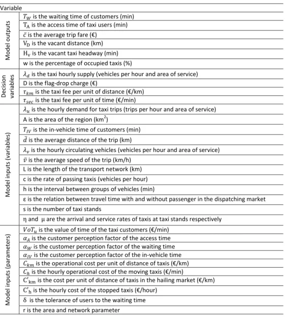
The principal variables and parameters considered in the taxi models presented in the literature are listed and defined in Table 1.

Table 1 Variables definition Variable Mod el o u tp u ts

ܶௐ is the waiting time of customers (min)

୅ is the access time of taxi users (min)

ܿҧ is the average trip fare (€)

ୈ is the vacant distance (km)

୴ is the vacant taxi headway (min)

w is the percentage of occupied taxis (%)

De

cision

variables

ߣௗ is the taxi hourly supply (vehicles per hour and area of service)

D is the flag-drop charge (€)

߬௞௠ is the taxi fee per unit of distance (€/km)

߬௦௘௖ is the taxi fee per unit of time (€/min)

M o del i n put s ( va ria ble s)

ߣ௨ is the hourly demand for taxi trips (trips per hour and area of service)

A is the area of the region (km2)

ܶூ௏ is the in-vehicle time of customers (min)

݀ҧ is the average distance of the trip (km)

ߣ௩ is the hourly circulating vehicles (vehicles per hour and area of service)

ݒҧ is the average speed of the trip (km/h) L is the length of the transport network (km) c is the rate of passing taxis (vehicles per hour) h is the interval between groups of vehicles (min)

ε is the relation between travel time with and without passenger in the dispatching market s is the number of taxi stands

Ʉ and Ɋ are the arrival and service rates of taxis at taxi stands respectively

Mod el inp u ts ( p aramete rs)

ܸ݋ܶ௨ is the value of time of the taxi customers (€/min)

ߙ஺ is the customer perception factor of the access time

ߙௐ is the customer perception factor of the waiting time

ߙூ௏ is the customer perception factor of the in-vehicle time

ܥ௞௠ is the operational cost per unit of distance of taxis (€/km)

ܥ௛ is the hourly operational cost of the moving taxis (€/min)

Ԣ୩୫ is the cost per unit of distance of taxis in the hailing market (€/km)

Ԣ୦ is the hourly cost of the stopped taxis (€/hour)

Ɂ is the tolerance of users to the waiting time r is the area and network parameter

The following sub-chapters aim at presenting the formulations proposed by the various authors in the literature. An extensive review of the models can be found in Salanova et al. (2011).

(4)

2.2.The demand for taxi trips

The demand for taxi trips depends on both the socioeconomic characteristics of the population and the comparison between the characteristics of the taxi service and the alternative transport modes. Various formulations can be found in the literature (Yang et al. 2001, Yang et al. 2005, Schroeter 1983), mostly using the expected waiting time or the number of vacant taxis and the relative or absolute cost of the trip. The more recent models propose the use of searching and meeting function between customers and taxi drivers, where the taxi driver searches for a ride taking into account the searching time and the ride revenue while the customer searches for a taxi ride trying to minimize the generalized cost of his/her trip.

Wong et al. (2001) consider separate demand functions for each OD pair (i, j), depending on customer waiting time in zone i (_୛௜), trip price (ܿҧ௜௝) and travel time (୍୚௜௝) between zones i and j. They use an exponential function for

expressing customer demand from zone ݅ to zone ݆ (ߣ_௨௜௝) as it is shown in Equation 1.

ߣ_௨௜௝ൌ ܦ෩௜௝൉ ݁ିఊሺ௖ҧ೔ೕାఈ಺ೇή௏௢்ή்಺ೇ೔ೕାఈೈή௏௢்ή்ೈ೔ሻ ሺͳሻ

Where ܦ෩௜௝ is the potential demand from zone i to zone j and ߛ is the scaling parameter.

Daniel (2003) modeled a taxi market in which fare and entry are regulated and tested using the data obtained by Schaller (2007) and found an inelastic relationship between vacant taxicabs and demand. In his work, a demand function is used, depending on the price of the service (ܿҧ) and the number of vacant taxi cabs (V).

ߣ௨ൌܿҧఉܸఊܺ஽ ሺʹሻ

where γ and β are the elasticities of price and demand respectively and XD is a function of exogenous variables.

The use of a modal split will make more complex the model since detailed data for each OD pair is needed for the taxi services and for all the alternative modes. Two examples of the modal split calculation are presented in Lo and Yip (2001), where the authors applied a Multinomial Logit Model to the transit services, and in Wong et al. (2005). An example is the demand formulation proposed by Chang and Chu (2009), where the demand rate (ߣ_௨) is calculated as in Equation 3:

ߣ௨ܣ ൌ

ܦܿҧఈ_ܶ ௐఉ

݀ҧ ሺ͵ሻ

where D, α and β are calibrated parameters of the model.

2.3.Trip cost

Chang et al. (2010) propose the following formulation for estimating the willingness to pay of taxi users (ܲ):

ܲ ൌ ܲ଴െ ܸ݋ܶ ൉ ܶ௪ఋെ ݑ ሺͶሻ

(5)

at a rate controlled by Ɂ where ݑ is the communication cost. An interesting discussion on various user classes with different values of time can be found in Wong et al (2004). Many studies have obtained specific values for the VoT of the citizens by trip purpose, trip length, income and others. For the value of time, Small (1992) proposed the 50% of the average hourly salary, while Daganzo (2010) assumes it to be 20$/hour.

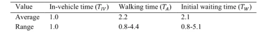
Three weighting parameters are used in order to use a unique VoT for the taxi users. The parameters weight access time, waiting time and in-vehicle travel time, taking into account the users’ perception of the time for each case. There is the need for calibrate the parameters in each city and society. While Kittelson et al. (2003) proposed the values presented in Table 2.

Table 2 – Relative Importance of TravelTime Components for Work Trips. Kittelson et al. (2003).

Value In-vehicle time (ܶூ௏) Walking time (ܶ஺) Initial waiting time (ܶௐ)

Average 1.0 2.2 2.1

Range 1.0 0.8-4.4 0.8-5.1

These values should be adapted to each region. Recently, Raveau et al. (2011) have obtained similar values for the metro of the city of London (one minute of waiting equal to 1.07 minutes of travel and one minute of walking equal to 1.79 minutes of travel).

2.4.The taxi supply and the vacant distance

The supply for taxi services depends on the expected benefit when offered to the users. There exists an opportunity cost for both the license holder and the taxi driver. The license holder has invested money in the license and expects high revenues from his investment, while the taxi driver invests his own time in exchange for a salary. In macroeconomic terms the supply depends on the revenues and salary, related to alternative revenues and salaries, however, in most of the models the supply depends on the revenues as an absolute value and not in relation to the other economic sectors. An important variable for the supply side is the vacant distance; in the stand market it is equal to the distance between the destination of the customer and the nearest taxi stand. In the dispatching market the vacant distance is equal to the distance between the stand and the customer´s origin, and between the customer´s destination and the nearest stand (both supposed to be equal in most of the models). In the hailing market the vacant distance can be approximated by the difference between the distance travelled by the taxis during one hour (ߣ_ௗݒҧ) and the distance travelled by the customers during one hour (ߣ௨݀ҧ).

ܸ஽ൌ ߣௗܣݒҧ െ ܣߣ௨݀ҧ

(5)

Chang et al. (2010) propose the following formulation for the estimation of the vacancy mileage per taxi in the dispatching market:

ܸ஽ൌ ʹ

ܣଵൗଶ_ݎ

Ͷݏఏ ሺ͸ሻ

where Ʌ is the stand allocation coefficient.

Yang et al. (2005) relate the fleet size (vacant and occupied) to the demand and the travel time, where the occupied taxi fleet is calculated from the total travelling time of all customers. Another approach presented in the literature is to calculate the supply as the optimum fleet related to the minimum cost. Chang et al. (2010) presents the following

(6)

formulation for calculating the optimum fleet for the hailing market: ߣௗכൌ ܮ ݒҧ቎ቆ ͳʹͲఋ_{൉ ܸ݋ܶ ൉ ߜ ൉ ߣ} ௨ ܥԢ௞௠ܣఋାଵ ቇ ଵ ఋାଵ ൅ ߣ௨݀ҧ቏ ሺ͹ሻ

Daganzo (2013) was the first to study the travel and waiting time as physical variables. In his work the optimal size of the taxi fleet using the queue theory is studied and a region where dispatching services are offered to customers is considered. Daganzo (2013) analysed the three states of the dispatching taxies (idle, assigned and servicing), and the number of taxis in each state and formulated the problem as in Equation 8:

ߣௗכൌͳǤʹߣ௨ଶȀଷݒҧିଶȀଷ൅ߣ௨

ݒҧ

ሺͺሻ

2.5.Access and waiting time

In the hailing and dispatching markets the access time is either 0 or very small. In the case of the stand market, as proposed in Zamora (1996) the access distance can be approximated by s/2, where s is the length of the squares generated by an orthogonal stand network with constant spacing. The models of Yang et al. (2005) and Chang and Chu (2009) use the number of available taxis for obtaining the customers waiting time. In the dispatching market, the average waiting time can be expressed in terms of reaction time (negligible) and taxi access time. The customer waiting time is the average taxi travel time between the customer and the nearest vehicle, related to the density of free taxis in the area. The proposed formulation in Zamora (1996) is:

ܶ௪ൌ ͲǡͶݎ ݒҧඨߣௗെ ߣ௨ݎܣ ଵ ଶ ൗ ʹݒҧ ߝ ሺͻሻ

Daganzo (2013) proposes the following formulation for the waiting time in the dispatching market when the number of vehicles is the optimum.

ܶ௪ൌͲǤͺߣ௨ଵȀଷݒҧଶȀଷ ሺͳͲሻ

Chang et al. (2010) propose the following formulation for the waiting time in the dispatching market: ܶ௪ൌ

ܸ஽Ȁʹ

ݒҧ ൅ ܶ ሺͳͳሻ

where T is the waiting time for central dispatching center.

Meyer and Wolfe (1961) presented a very detailed formulation for the estimation of the waiting time in the dispatching market. They presented and analyzed the complex case where customers have to wait until the first

(7)

occupied taxi is available, increasing the waiting time and reducing the LoS. In the hailing market, Wong et al. (2004) use the number of vacant taxis and the size of the area of service for calculating the waiting time, assuming a continuous taxi stand distribution. Using a more statistical approach, the waiting time is equal to the time that the user must wait until the first free taxi reaches the customer, starting from a random moment when the user decides to take a taxi. Another interesting approach is presented in Bautista (1985). Considering that taxis are passing by a concrete point of the network at constant intervals (c), the expected waiting time is equal to the number of taxis that have passed before the first free taxi multiplied by the interval time between them.

ܶ௪ൌ

ሺߣ௩൅ሻ

ሺʹߣ௩ሺߣ௩Ǧሻሻ

(12)

Considering that the taxis follow an exponential distribution with an average of 1/c, the waiting time can be expressed as proposed by Bautista (1985):

ܶ௪ൌ

ͳ

ሺሺߣ௩Ǧሻሻ ሺͳ͵ሻ

Adding the fact that in cities vehicles tend to move in platoons (due to the traffic lights), the waiting time can be estimated as proposed by Bautista (1985):

ܶ௪ൌ

݄ ʹ

ͳ ൅ ݁ݔ݌ሺെ݄ܿሺߣ௩െሻሻ

ͳ െ ݁ݔ݌ሺെ݄ܿሺߣ௩െሻሻ

(14)

In the stand market, the waiting time can be estimated by applying queue theory to a double queue, where vehicles and users meet each other (Yang et al (2010a and 2010b) and Matsushima and Kobayashi (2006 and 2010)). Lo and Yip (2001) propose the following formulation for the calculation of the user waiting time at taxi stands.

ܶ௪ ൌ

ͳ

ߤሺͳ െ ߟ ߤൗ ሻ ሺͳͷሻ

Yang et al (2000) proposed the following formulation for the waiting time at a taxi stand: ܶ௪ൌ ܤ ൬

ͳ ܪ௩൰ ൅ ܥ ൬

ߣ௨

ߣௗ൰ ሺͳ͸ሻ

where B and C are empirical parameters of the model, calibrated by the authors with data from the taxi fleet of Hong Kong. The vacant taxi headway is estimated in Yang et al (2000) using the percentage of occupied taxis.

2.6.In-vehicle travel time

The in-vehicle travel time is the same for the hailing and dispatching modes. It can be expressed by using the average distance between two interior points within the zone and the average speed, as shown in Zamora (1996).

(8)

ܶூ௏ൌ

ݎܣଵൗଶ

ʹݒҧ ሺͳ͹ሻ

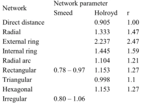
Paremeter r is the ratio between the real distance (network distance) and the Euclidean distance, which depends on the network geometry. Smeed (1975) and Holroyd (1965) calculated various r values for nine network configurations, presented in Table 3.

Table 3 – Network parameters proposed by Smeed and Holroyd. Zamora (1996)

Network Network parameter

Smeed Holroyd r Direct distance 0.905 1.00 Radial 1.333 1.47 External ring 2.237 2.47 Internal ring 1.445 1.59 Radial arc 1.104 1.21 Rectangular 0.78 – 0.97 1.153 1.27 Triangular 0.998 1.1 Hexagonal 1.153 1.27 Irregular 0.80 – 1.06

In the stand mode the in-vehicle travel time is equal to the travel time between the users destination and the nearest to the users’ origin taxi stand.

2.7.Costs

In the dispatching market the unitary driver cost depends on the number of taxis stopped at taxi stands and the number of taxis cruising the streets (Zamora (1996)). For the cruising taxis, the unitary operation cost per passenger is the following:

ݖௗ = _ఒఒ೏

ೠܥ௛+

୰୅భൗమ

2௩ത ߳ܥ௞௠ (18)

For the stopped taxis, the unitary driver operation cost is expressed by Zamora (1996) as:

ݖௗൌ ߣௗെ ߣ௨ݎܣ ଵ ଶ ൗ ʹݒҧ ߳ ߣ௨ ܥԢ௛ ሺͳͻሻ

The unitary cost of drivers in the stand market is very similar to the unitary costs of the stopped taxis in the dispatching market, with the only difference of access distance being 0 (߳ ൌ ͳ). In the hailing market, unitary cost can be expressed as:

ݖ

ௗ

=

ఒ_ఒ೏ ೠ

ܥ

௛

+

ఒ_೏௩ത

ఒ_ೠ

ܥ

௞௠

(20)

For the dispatching market, Chang et al. (2010) present cost formulation for passengers, drivers and operators. The passengers total cost is composed by the cost of communications, the product between the waiting time (half vacant time since the distance between the customer´s origin/destination and the nearest taxi stand are supposed to be

(9)

equal) and the value of time, and finally the time needed for the control centre to dispatch vehicles (T). ܼ௨ൌ ൉ ߣ௨൉ ൉ ൅

൉ ୈ

ʹݒҧ ൅ ൉ ߣ௨൉ ൉ ൉ (21)

The driver cost includes both the occupied and vacant distances.

ܼௗൌ ܥ௞௠൉ ߣ௨൉ ൉ ݀ҧ ൅ ܥ௞௠൉ ୈ (22)

The operator cost is supposed non-linear and calculated as the marginal cost of each taxi stand multiplied by the number of taxi stands.

ൌ ൬ߣௗ ൰

ఊ

(23) where γ is the incremental operating cost coefficient of taxi stand (0<γ<1) and b is the marginal operation cost. The average stand cost can be obtained as the sum of the fixed cost (negligible) and the variable costs. The variable costs are a function of the number of offered places. It is shown in Zamora (1996) that the optimum number of places per stand is one, and the only issue is to find the optimum number of stands (s*). The proposed formulation presented in Zamora (1996) is the following:

כ₌_ߣ ௗ െ ߣ௨ ଵൗଶ 2ݒҧ ɂ ൅ ൮ ͲǤͷሺܥ௛െ ܥԢ௛ሻͲǤͶߣ௨ଶൗଷ ݒҧ ɔ ൲ ଶ ଷ ൗ (24)

where φ is the opportunity cost of having a taxi reserved place (€/hour)

3.Conclusions

As shown in this paper there are detailed formulations in the literature for estimating the different variables of the taxi market for all operating modes. Scientific contributions in the taxi management agree on the most important variables for modelling the taxi market, such as waiting time, generalized cost or optimum fleet, presenting similar formulations. However, each author proposes his/her own generalized cost and the related optimum fleet. There is a need for developing a unique model able to be used for the three operation modes. Most authors studied the dispatching market, where taxis wait at taxi stands for a call. There was a need for further research on the other two operating modes (hailing and stand), especially in the hailing market, since the variables’ formulation is much more complex. Also, combined markets need to be modelled, with heterogeneous taxi fleets composed by the three mentioned markets.

All the presented models need to be calibrated with real world or simulation data in order to understand the effects of the variables and to validate their hypotheses. Agent models such the one presented in Salanova et al. (2013) should also be developed for simulating the drivers’ and users’ behavior and support the proposed models with simulation data.

(10)

and at the same time the demand depends on the waiting time, forming a bi-level problem where the demand is obtained in the upper level and the waiting time associated to the demand is recalculated in the second level.

Acknowledgements

This work was supported by the ENTROPIA project, funded by the Spanish Ministry of Economy and Competitiveness. Non-oriented Fundamental Research Projects. CODe: TRA2012-39466-C02-01.

References

Bautista J. (1985). Models de distribució del temps d’espera del taxi. Tesina final de carrera. ETSEI Barcelona.

Chang S. K. and Chu-Hsiao C. (2009). Taxi vacancy rate, fare and subsidy with maximum social willingness-to-pay under log-linear demand

function. Transportation Research Record: Journal of the Transportation Research Board, 2111 pp. 90 – 99.

Chang S. K. J., Wu C. H., Wang K. Y. and Lin C. H. (2010). Comparison of Environmental Benefits between Satellite Scheduled Dispatching and Cruising Taxi Services. Proceedings of the TRB Annual Meeting.

Daganzo C. F. (2013) Lesson notes (available at http://www.ce.berkeley.edu/~daganzo/index.htm).

Daganzo C. F. (2010). Structure of competitive transit networks. Transportation Research Part B 44, pp. 434-446.

Daniel F.G. (2003) An Ecomic Analysis of Regulated Taxicab Markets. Review of Industrial Organization 23, pp. 255 – 266.

Holroyd E. M. (1965). The optimum bus service: a theoretical model for a large uniform urban area. In L. C. Edie, R. Herman, and R. Rothery (Eds.), Vehicular Traffic Science, Proceedings of the 3rd International Symposium on the Theory of Traffic Flow. New York: Elsevier. Kittelson & Associates. (2003). Transit Capacity and Quality of Service Manual. Transit cooperative research program report 100, 2nd Edition. LO H. K. and YIP C. W. (2001). Fare deregulation of transit services: winners and losers in a competitive market. Journal of Advanced

Transportation, 35 (3) pp. 215 – 235.

Matsushima K. and Kobayashi K. (2006) Endogeus market formation with matching externality: an implication for taxi spot markets. Structural

Change in Transportation and Communications in the Kwledge Ecomy, pp. 313 – 336.

Matsushima K. and Kobayashi K. (2010) Spatial equilibrium of taxi spot markets and social welfare. 12th World Conference of Transport Research, Lisbon, Portugal.

Meyer, R. F. and Wolfe, H. B. (1961), The organization and operation of a taxi fleet. Naval Research Logistics Quarterly, 8 pp. 137–150.

Raveau S., Muñoz J. C. and DE Grange L. (2011) A topological route choice model for metro. Transportation Research Part A 45 (2), pp.

138-147.

Salanova J. M., Estrada M., Aifadopoulou G. and MITSAKIS E., (2011). A review of the modeling of taxi services. Procedia and Social Behavioral Sciences 20, pp 150-161.

Salanova J.M., Estrada M. A., Mitsakis E. and Stamos I. “Agent Based Modeling for Simulation of Taxi Services”. Journal of Traffic and

Logistics Engineering (JTLE) (ISSN: 2301-3680), 1 (2), June 2013. pp. 159 – 163, 2013.

Schaller B. (2007). Entry controls in taxi regulation: Implications of US and Canadian experience for taxi regulation and deregulation. Transport

Policy 14, pp 490 – 506.

Schroeter J. R. (1983). A model of taxi service under fare structure and fleet size regulation. The Rand Company, The Bell Journal of Ecomics,

14, 1, pp 81 – 96.

Small, K. (1992). Using the revenues from congestion pricing. Transportation, 19, pp. 359–381.

Smeed, R. J. (1975). Traffic studies and urban congestion.

Wong K. I., Wong S. C. C.O. Tong, W. H. K. Lam, H. K. LO, Yang H. and H. P. Lo (2005). Estimation of origin-destination matrices for a multimodal public transit network. Journal of Advanced Transportation, 39 (2), pp. 139 - 168.

Wong K. I., Wong S. C., Wu J.H., Yang H. and Lam W.H.K. (2004). A combined distribution, hierarchical mode choice, and assignment network model with multiple user and mode classes. Urban and regional transportation modeling.

Wong K. I., Wong S. C. and Yang H. (2001). Modeling urban taxi services in congested road networks with elastic demand. Transport Research

B 35, pp. 819 – 842.

Yang H., Cowina W. Y. L., Wong S. C. and Bell M. G. H. (2010b). Equilibria of bilateral taxi-customer searching and meeting on networks.

Transport Research B 44, pp. 1067 – 1083.

Yang H., Fung C. S., Wong K. I. and Wong S. C. (2010a). nlinear pricing of taxi services. Transport Research A 44, pp. 337 – 348.

Yang H., Wong K. I. and Wong S. C. (2001). Modelling Urban Taxi Services in Road Networks: Progress, Problem and Prospect. Journal of

Advanced Transportation 35 (3), pp. 237 – 258.

Yang H., Yan Wing Lau, Sze Chun Wong and Hong Kam Lo (2000). A macroscopic taxi model for passenger demand, taxi utilization and level of services. Transportation 27, pp. 317-340.

Yang H., Ye M., Tang W. H. and Wong S. C. (2005). Regulating taxi services in the presence of congestion externality. Transport Research A 39,

pp. 17 – 40.