INSTITUTE FOR
PARALLEL AND
DISTRIBUTED
SYSTEMS
S
IMULATION
T
ECHNOLOGY DEGREE COURSE
Master’s Thesis
Submitted to the University of Stuttgart
Efficient Algorithms for
Geodesic Shooting in Diffeomorphic
Image Registration
Examiner
Prof. Dr. Miriam MEHL Institute for Parallel and Distributed Systems
Supervisor
Dr. Ing. Andreas MANG Department of Mathematics, University of Houston, USA
Submitted by
Abstract
Diffeomorphic image registration is a common problem in medical image analysis. Here, one searches for a diffeomorphic deformation that maps one image (the moving or template image) onto another image (the fixed or reference image). We can formulate the search for such a map as a PDE constrained optimization problem. These types of problems are computationally expensive. This gives rise to the need for efficient algorithms.
After introducing the PDE constrained optimization problem, we derive the first and second order optimality conditions. We discretize the problem using a pseudo-spectral discretization in space and consider Heun’s method and the semi-Lagrangian method for the time integration of the PDEs that appear in the optimality system. To solve this optimization problem, we consider an L-BFGS and an inexact Gauss-Newton-Krylov method. To reduce the cost of solving the linear system that arises in Newton-type methods, we investigate different preconditioners. They exploit the structure of the Hessian, and use algorithms to efficiently compute an approximation to its inverse. Further, we build the preconditioners on a coarse grid to further reduce computational costs.
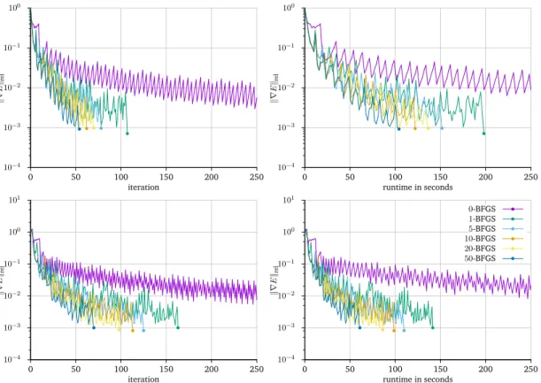
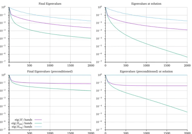
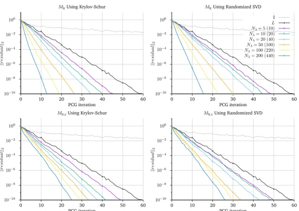
The different methods are evaluated for two-dimensional image data (real and synthetic). We study the spectrum of the different building blocks that appear in the Hessian. It is demonstrated that low rank preconditioners are able to significantly reduce the number of iterations needed to solve the linear system in Newton-type optimizers. We then compare different optimization methods based on their overall performance. This includes the accuracy and time-to-solution. L-BFGS turns out to be the best method, in terms of runtime, if we solve solving for large gradient tolerances. If we are interested in computing accurate solutions with a small gradient norm, an inexact Gauss-Newton-Krylov optimizer with the regularization term as preconditioner performs best.
Acknowledgments
This work was supported by a fellowship within the FITweltweit program of the German Academic Exchange Service (DAAD). Without this scholarship this thesis would not have been possible.
Contents
1 Image Registration 11
1.1 Overview . . . 11
1.2 Own Contribution and Thesis Outline . . . 12
1.3 Related Work . . . 13
2 Geodesic Shooting 15 3 Optimization 19 3.1 Iterative Optimization Methods . . . 19
3.1.1 Gradient Descent . . . 19
3.1.2 Newton’s Method . . . 20
3.1.3 Gauss-Newton . . . 20
3.1.4 BFGS and L-BFGS . . . 21
3.2 Optimize-then-Discretize . . . 21
3.3 Gradient of the Optimization Functional . . . 21
3.3.1 Vector Valued Momentum . . . 22
3.3.2 Scalar Valued Momentum . . . 23
3.4 Hessian of the Optimization Functional . . . 24
3.4.1 Vector Valued Momentum . . . 25
3.4.2 Scalar Valued Momentum . . . 26
3.5 Summary . . . 26
4 Discretization 29 4.1 Spatial Discretization . . . 29
4.1.1 Discretization of the Optimization Functional . . . 29
4.1.2 Grid Transfer Operations – Prolongation and Restriction . . . 30
4.2 Temporal Discretization . . . 30
4.2.1 Heun’s Method . . . 31
4.2.2 Semi-Lagrangian Method . . . 31
4.3 Krylov Subspace Solver . . . 34
4.4 Summary . . . 34
5 Preconditioners 35 5.1 Inverse Regularization Term . . . 35
Contents
5.3 Low Rank Approximation . . . 37
5.4 Low Rank Approximation on Coarse Grid . . . 38
5.5 Randomized Low Rank Approximation . . . 38
5.6 Summary . . . 39 6 Numerical Results 41 6.1 Performance Metrics . . . 41 6.1.1 Optimization Methods . . . 41 6.1.2 Preconditioners . . . 43 6.2 General Convergence . . . 44 6.3 L-BFGS Convergence . . . 45
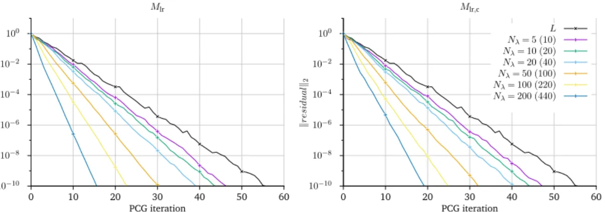
6.4 Spectral Properties of the Hessian and Low Rank Approximation . . . 46
6.4.1 Decay of Eigenvalues . . . 47
Coarse Grid . . . 48
Convergence at the Solution and Expansion Length . . . 49
6.4.2 Resolution Independence . . . 52
6.5 Preconditioner for Newton’s Method . . . 52
6.6 Comparison of L-BFGS and Newton Methods . . . 52
6.7 Using the Semi-Lagrangian-Method . . . 54
6.8 Summary . . . 55
7 Outlook 57
Bibliography 59
Nomenclature
advm (∇v)m−(∇m)v
ad†
v adjoint operator ofadv.ad†vm= (∇v)Tm+ (∇m)v+vdiv(m)
L† adjoint of operatorL
β regularization parameter
diagi=1,...,n(ai) diagonal matrixA∈Rn×nwithAi,i=ai
divf =∇ ·f divergence of a vector valued function, only in spatial dimensions
E objective functional
Eh discretized objective functional
Ff Fourier transformation of f
gradf=∇f gradient of a function, only in spatial dimensions
H Hessian
Hc Hessian on a coarser discretization
Hmis mismatch term of the HessianH=βHreg+Hmis
Hreg regularization term of the HessianH=βHreg+Hmis
ht time step size
hx discretization width in each spatial dimension
I identity map I(x) :=xor matrix Ix:=x
L−1 inverse of operatorL
K inverse ofL: v=Km
Contents
Mlr−1 preconditioner using a low-rank approxiation of the mismatch term
Mlr−,1c Mlrpreconditioner build on a coarser discretization
Nx number of nodes in each spacial dimension
AT transpose of matrixA
BFGS Broyden–Fletcher–Goldfarb–Shanno algorithm
CFL Courant-Friedrichs-Lewy condition
CG conjugate gradient method
FFT Fast-Fourier-Transform
FN (full) Newton’s method
GD gradient descent
GMRES generalized minimal residual method
GN Gauss-Newton
L-BFGS Limited memory BFGS algorithm
LDDMM large deformation diffeomorphic metric mapping
PCG preconditioned conjugate gradient method
PDE partial differential equation
1 Image Registration
Image registration is aninverse problem. It involves the process of finding a mapφthat describes how a template image I0 can be deformed to resemble a reference image I1
in some sense [42]. This problem often arises in medical image analysis. Common examples include the registration of magnetic resonance imaging (MRI) scans onto a standardized template, normalizing time series of images, the reconstruction of a 3D model from multiple MRI scan slices or combining images from multiple measuring techniques [41, 42, 20, 49].
1.1 Overview
Given two imagesI0: Ω→RandI1: Ω→Rwe try to find a functionφ: Ω→Ωthat maps the first image onto the second so thatI0◦φ−1≈I1. The image domainΩis a compact
subset ofRdford∈ {2,3}. Furthermore, we want to restrict admissible functions forφ to be diffeomorphisms. Using diffeomorphisms ensures that structures do not vanish, no folding is introduced and that neighborhood structures are preserved. In general, this problem is ill-posed [20]. The solution is not guaranteed to be unique as different mappings can yield the same or very similar results. Moreover, small perturbations in the images may lead to vastly different solutions. A strategy to overcome ill-posedness is to introduce a regularization model [19]. Consequently, the optimization problem consists of two term: a mismatch term and a regularizer. The mismatch term measures the fidelity of the deformed template imageI0◦φ−1and the reference imageI1. The regularization
term favors diffeomorphisms that are close to the identity in a predefined the metric [39]. It is not immediately clear, how one can minimize over the group of diffeomorphisms. One option is to introduce an artificial time variablet∈[0,1]and use a time dependent velocity fieldvand obtain the associated diffeomorphismφ: Ω×[0,1]→Ωas the solution of the differential equation∂tφ(x, t) =v(φ(x, t), t)whereφ(x,0) =x[52, 53, 17, 39, 56].
Under certain smoothness requirements onvit follows thatφis a diffeomorphism [17, 46] and therefore admissible for the matching problem(I0◦φ−1)(·,1)≈I1(·). This leaves us
with a well posed problem [17].
Usingvas a control variable, the problem can be reformulated so that we search for a smooth time dependent velocity field. Furthermore, it can be shown that the minimizing velocity field satisfies an Euler-Lagrange-Equation, which defines the evolution ofvover
1 Image Registration
time [39, 40]. This allows us to reduce the optimization space to the initial conditions of the Euler-Lagrange-Equation. In analogy to shooting a projectile into the air, where the trajectory is defined by the initial angle, velocity and physical laws, this method leads to a so calledgeodesic shooting method: The evolution of the velocity (and with it the diffeomorphism) is described by an initial velocity and the Euler-Lagrange-Equation. Given the minimization functional we can now state an optimization problem that is constrained by the Euler-Lagrange-Equation. This problem can be solved using a gradient descent method or Newton’s method. While Newton’s methods should give better convergence rates, it also requires matrix-vector-products with the inverse of the Hessian of the minimization functionalH−1. Direct methods to invertHare in general
not applicable as forming and and storingH is too expensive and not possible. Hence, we will consider iterative methods instead. To improve the convergence rate of the linear solver and reduce the computational effort needed in each Newton step, we are interested in efficient preconditioners.
1.2 Own Contribution and Thesis Outline
This work is based on the OCREG code [32, 33, 34] for diffeomorphic image registration. In this work the code has been extended by the geodesic shooting formulation for scalar and vector valued momentums, the corresponding gradients and Hessians for the optimization, a L-BFGS optimizer and different preconditioners for Newton’s method. Starting with chapter 2 we show how the PDE constrained minimization problem for geodesic shooting can be derived from a mismatch term and the requirement that the final mappingφis a diffeomorphism.
In chapter 3 we reformulate the constrained minimization problem as an unconstrained minimization problem. We shortly discuss different optimization methods, which can be used and derive the necessary gradient and Hessian.
These expressions are then discretized in chapter 4. We discuss the spatial and temporal discretization. We also show how the PDEs arising in the gradient and Hessian expressions can be solved using Heun’s method or a semi-Lagrangian scheme.
In chapter 5 we introduce a new preconditioner which can be used in the linear solver needed in Newton-type optimizers. This preconditioner is based on a low rank approxi-mation of the Hessian and only requires matrix-vector-products during its setup. Hence, it is matrix free and does not require knowledge of individual matrix entries. Furthermore, it can be build on a coarser discretization.
We evaluate the efficiency of the preconditioner in chapter 6. We evaluate the precon-ditioner on its own based on its ability to reduce the costs of solving the linear Hessian system and based on its efficiency during the entire registration process. Furthermore, we compare the results of the Newton optimizers against L-BFGS optimizers.
1.3 Related Work
1.3 Related Work
The image registration problem is often solved by minimizing a functional E=Ereg+Emis
which consists of a mismatch termEmisand a regularization termEreg[42]. The mismatch
term defines how we measure the mismatch between two images. The regularization term usually enforces some type of smoothness on the solution to ensure well-posedness of the minimization problem [20]. Because a specific regularization term also implies what kind of solution is expected, a vast variety of different regularizers have been proposed for different problems [20, 42, 46].
In this work, we want to focus on registration problems with large deformations.
There-fore, we use large deformation diffeomorphic metric mapping(LDDMM) methods [6].
To allow for large deformations, an artificial time variablet∈[0,1]is introduced. The transformation of the image happens gradually over time. Early work goes back to [12], which models the transformation as an evolving fluid. Furthermore, we are interested
in diffeomorphic maps, which ensures that the computed map φ is a bijections with
a smooth inverse [3]. Diffeomorphic maps can be obtained by inverting for a time dependent velocity field subject to certain smoothness requirements [17] which leads to a PDE constrained optimization problem [6]. The minimization problem can be seen as a shortest path problem or path of minimal energy problem in the space of diffeomorphisms and defines a metric in this space [39, 6].
Geodesic shooting methods, such as [40, 54], only invert for an initial value instead
of solving for a time dependent velocity field. The initial value combined with an additional PDE constraint on the minimization problem fully describe the evolution of the diffeomorphism over time.
Optimizations methods for the discretized LDDMM problem often involve first order methods such as the gradient descent method. LDDMM was initially presented in [6] to invert for a velocity field and is based on the theoretical results described in [52, 53]. Different gradient descent method for a shooting formulation has been presented in [54, 57]. Second order methods have been explored in [5, 24, 23, 32, 33, 35, 38, 34, 36], among others. [32] uses a preconditioned Newton-Krylov method to invert for a time dependent velocity field. [55] uses the Hessian matrix with respect to a vector valued initial momentum to estimate uncertainties in regularization parameters.
Because second order methods usually involve the solutions of a linear system, pre-conditioners can greatly improve the efficiency of such methods. Common choices for preconditioners include the inverse regularization operator [45, 32, 2, 37]. In [32] and [36] a two level preconditioner is proposed to invert for a velocity field. Further preconditioners have been discussed in [7, 48].
2 Geodesic Shooting
This introduction is mostly based on the work of [39, 40, 59], which provide a good overview of this topic. Another good introduction can be found in [58]. As mentioned before the regularization term favors diffeomorphisms close to the identity. This is done by penalizing the geodesic length of the path between the identity and the final diffeomorphism. Because the gradual evolution of the diffeomorphism is described by the velocity fieldv, the geodesic length is measured by integrating the velocity in a chosen normk·kV over the artificial timet∈[0,1]:
Ereg(φ) :=
Z 1
0 kv(·, t)k
2
V dt.
The norm of the velocity field is usually chosen to be a norm of a Sobolev space and defined as
kvk2V :=hv, LviL2
with linear differential operatorL. The differential operator has to be chosen so that the velocities are sufficiently smooth and thus give rise to a diffeomorphism [17, 46]. The required smoothness depends on the number of dimensions of the image domain. A common choice isL= (I−∆)γ withγ >0 [39, 55, 46]. Using the second Sobolev
embedding theorem one can show that for two dimensional imagesγ >2is sufficient [46]. The shortest geodesic path between two diffeomorphisms satisfies the so-calledEPDiff equation
0 =∂tm+ ad†vm, (2.1)
which is the Euler-Lagrange-equation for the corresponding variational problem for the
momentumm=Lv. Solutions to this PDE are calledgeodesics.
It can be shown that the minimizer to the registration problem v∗= argmin v 1 2β Z 1 0 kv(·, t)k 2 V dt+Emis(I1, I(1)) subject to 0 =∂tI+v· ∇I
2 Geodesic Shooting
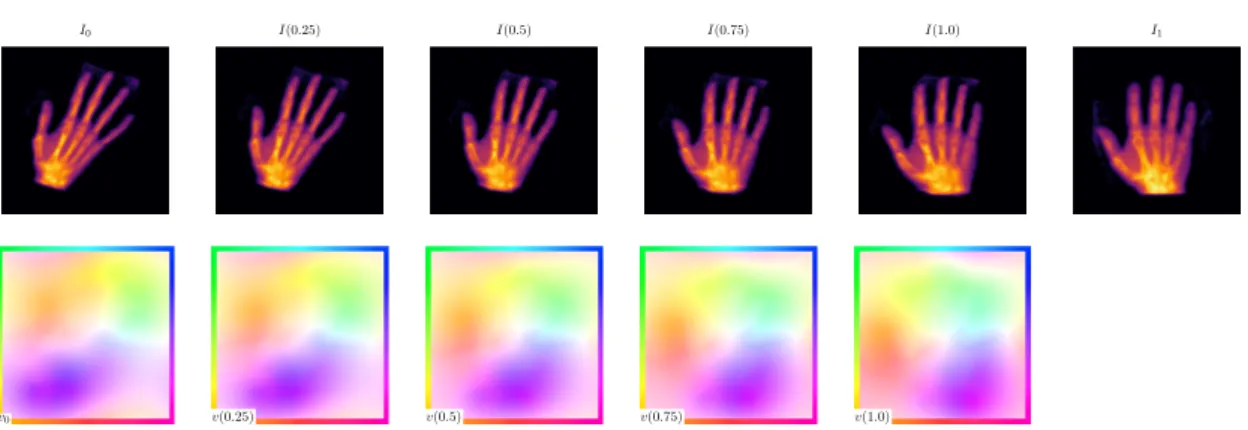
I0 I(0.25) I(0.5) I(0.75) I(1.0) I1
vv00 vv(0(0..25)25) vv(0(0..5)5) vv(0(0..75)75) vv(1(1..0)0)
Figure 2.1:Evolution of the image (top) and the velocity field (bottom) over time. is a geodesic and satisfies (2.1). This motivates the use of shooting methods. Because an initial velocity together with the EPDiff equation fully describes a geodesic, the minimization can be stated in terms of an initial velocityv0 and the EPdiff (2.1). The
minimization problem then reads v∗0= argmin v0 1 2β Z 1 0 kv(·, t)k 2 V dt+Emis(I1, I(1)) subject to 0 =∂tI+v· ∇I I(0) =I0 0 =∂tm+ ad†vm m(0) =L−1v0 0 =m−Lv.
The second constraint is the EPDiff equation and the third constraint is the definition
of the momentum. Together withv=Km, where K:=L−1, the EPDiff describes the
evolution of the velocity along the geodesic path. Figure 2.1 shows an example for the evolution of the velocity field along a geodesic.
Becausekv(·, t)kV is constant along a geodesic [54], the minimization functional can be
simplified into v∗0= argmin v0 1 2βkv0k2V +Emis(I1, I(1)) .
For the sake of simplicity, we will use aL2-mismatch term 1
2kI(1)−I1k
2
L2 throughout this
work. Reformulating the expression in terms of an initial momentumm0:=Lv0leads to
a constrained minimization problem.
Problem 2.1. Geodesic Shooting for Vector-Valued Momentum m∗0= argmin
m0
E(m0) (2.2)
with E(m0) = 1 2βhm0, Km0iL2+ 1 2kI(1)−I1k2L2 (2.3) subject to 0 =∂tI+v· ∇I I(0) =I0 (2.4) 0 =∂tm+ ad†vm m(0) =m0 0 =m−Lv.
Furthermore, it is shown in [6, Th. 2.1] that a minimizingm(t)is parallel to the image gradient∇I(t). Therefore, the minimization problem can also be stated in terms of a
scalar valued momentump[54].
Problem 2.2. Geodesic Shooting for Scalar-Valued Momentum p∗0= argmin p0 E(p0) (2.5) with E(p0) = 1 2βhp0∇I0, K(p0∇I0)iL2+ 1 2kI(1)−I1k2L2 (2.6) subject to 0 =∂tI+v· ∇I I(0) =I0 (2.7) 0 =∂tp+∇ ·(pv) p(0) =p0 0 =Lv−p∇I.
3 Optimization
In the previous chapter we derived the minimization problem. As a closed form solution to the problem is hard to find, we use iterative methods for minimization.
These methods depend on the gradient and the Hessian of the minimization problem with respect to the initial momentum. After giving a brief summary of different optimization methods, the following sections derive expressions for the gradient and the Hessian for both, a scalar and a vector valued initial momentum.
3.1 Iterative Optimization Methods
In the following sections we will see that the minimization problems 2.1 and 2.2 can be rewritten as an unconstrained minimization problem. Therefore, we briefly discuss different optimization methods for unconstrained optimization and how we use them in the optimization algorithm. For a more detailed explanation we refer to [44].
In the following we assume a minimization problem forf(x)with a sufficiently smooth functionf:Rn→R.
3.1.1 Gradient Descent
Gradient descent is a simple first order method, which only depends on the gradient of the minimization problem. In each iteration the current iteratexi is updated into the
direction of the negative gradient: xi+1=xi−αi∇f(xi),
with a step sizeαi>0[44]. Even though the negative gradient is a descend direction,
the step length is generally not known. Therefore, an additional line search is performed, which searches for a goodαi using additional function (and gradient) evaluations. As a
simple line search that ensures that each iteration reduces the minimization functionalf, we useArmijo backtracking[44, Ch. 3].
3 Optimization
3.1.2 Newton’s Method
Newton’s method is a second order method, which also requires the Hessian matrixH.
Based on a second order approximation, the Newton update reads [44] xi+1=xi−αiH−1∇f(xi).
In each step a linear system has to be solved. We use a preconditioned conjugate gradient method method (PCG) as discussed in section 4.3. Care has to be taken, as the direction
−H−1∇f(x
i)is not guaranteed to be a descend direction.
When the currentxiis still far from the solution, it is often not necessary to solve the linear
system to a high accuracy. This leads toinexact Newton Methods, where the tolerance for the residual norm decreases during the optimization process [44, Ch. 11].
In our experiments, we use an inexact Newton method with a quadratic forcing
se-quence[18] toli≤min 1 2,k∇ f(xi)k2 k∇f(x0)k2 !
for the tolerance of the residual normtoli in the linear solver.
To avoid problems with negative definite (negative curvature) or indefinite Hessians, we use an inexact Gauss-Newton method in most of our experiments.
3.1.3 Gauss-Newton
The Gauss-Newton method is a quasi-Newton method for minimization functionals of the formf(m0) =1/2Piri2(m0)[44]. The Hessian of such a functional reads
Hf = X i ∇ri·(∇ri)T+riHri ,
where Hr1 is the Hessian matrix of ri. The Gauss-Newton approximation drops the
second term containing the second order derivatives. In contrast to Newtons method, it can be shown that under certain constraints, the Gauss-Newton update is a descend direction [44].
To drop the second Hessian term in our formulation, we drop all term that multiply with the residualri. Asζ(1) =I1−I(1)is the residual, this corresponds to settingζ= 0in the
incremental adjoint equations which we derive in section 3.4. This causes the Hessian approximation to be positive semi-definite.
In our experiments we use an inexact Gauss-Newton method, where the tolerance for the residual normtolifollows asuper-linear forcing sequence
toli≤min 1 2, s k∇f(xi)k2 k∇f(x0)k2 ! . 20
3.2 Optimize-then-Discretize
3.1.4 BFGS and L-BFGS
BFGS and the memory limited version L-BFGS [43] quasi-Newton methods and perform a Newton update using approximations toH orH−1. Therefore, better convergence than
gradient descent can be expected [44]. Compared to Newton’s method, the approximate Hessian is much cheaper to compute, as it only needs gradient evaluations from previous iterations.
We use the two-loop algorithm [43, 44, Alg. 7.4] to approximate H−1 together with
Armijo backtracking as a line search method. To ensure the positive definiteness of the approximation we skip updates that do not satisfy the curvature condition. During our experiments, no updates had to be skipped.
3.2 Optimize-then-Discretize
To solve the optimization problem we follow aoptimize-then-discretizeapproach. This means that we use the continuous formulation of the optimization functional and first derive the corresponding gradient and Hessian in a continuous setting. We then discretize each term separately. This is in contrast to andiscretize-then-optimizeapproach where the optimization functional is discretized first, and the gradient and Hessian are derived from the discretized minimization functional. A more detailed discussion can be found in [21, 26]. An optimize-then-discretize implementations of LDDMM can be found in [32]. A discretize-then-optimize implementations is described in [38].
3.3 Gradient of the Optimization Functional
The constrained minimization problem for the geodesic shooting formulation (2.2) and (2.5) represents aoptimal control problem[26]. In such a setting one searches for an optimal control variable that minimizes a functional under the constraints of dynamical systems – the so called state equations. In the geodesic shooting problem the state equations define how the diffeomorphism evolves over time (by giving an evolution ofm orpand thereforev) and how the diffeomorphism acts on the initial image (by stating the evolution ofI).
The PDE constraints can be solved forward in time, which allows us to evaluate the objective functional for different initial momentums. Therefore, the most simple way to compute a gradient of the optimization problem is to use finite differences by evaluating the functional for different initial momentums. However, this implies that the constraints have to be solved very often if the initial momentum contains a large number of unknowns. This is usually the case for image data. A computationally cheaper approach is the so
3 Optimization
calledadjoint method[9, 26, Ch. 1.6]. It often allows to compute a gradient at much lower cost, independent of the number of unknowns.
For the adjoint method we first turn the PDE constrained problem into an unconstrained problem, using the method of Lagrangian multipliers [26, Ch. 1.6]. Based on the resulting Lagrangian we can compute the gradient with respect to the initial momentum. For this, we first have to solve the so-calledadjoint equation. This is often of similar cost to solving the state equations. The adjoint equations usually depend on the solution of the state equation. Each gradient evaluation includes solving the state and adjoint equations. For more details we refer to [26].
The resulting gradient can then be used in optimization methods like gradient descent.
3.3.1 Vector Valued Momentum
We now derive the gradient for the vector valued momentum following the previous outline. Based on the constrained minimization problem (2.2) the LagrangianLreads
L(m0, I, m, v, ζ, µ, ν) := 1 2βhm0, Km0iL2+ 1 2kI(1)−I1k2L2 (3.1) +Z 1 0 h ζ, ∂tI+v· ∇IiL2 dt+hζ(0), I(0)−I0iL2 +Z 1 0 D µ, ∂tm+ ad†vm E L2 dt+hµ(0), m(0)−m0iL2 +Z 1 0 h ν, m−LviL2dt,
where ζ, µ and ν are the Lagrangian multipliers for the state variables I, m and v, respectively. In this setting the Lagrangian multipliers are also called dual or adjoint
variables.
The next step is to compute the gradient of the Lagrangian, because a minimizer of the original problem is also minimizes the Lagrangian. The gradient can be found by computing directional derivatives for each control, state and adjoint variable. Taking the derivative of the Lagrangian with respect tom0 in the directionm˜0 gives
∂m0L[ ˜m0] =hβKm0−µ(0),m˜0iL2,
where we can read off the gradient
∇m0L=βKm0−µ(0). (3.2)
For a givenm0,Km0 can be easily computed. The expensive part is findingµatt= 0. To
evaluateµ(0)we have to solve the adjoint equation. The variations with respecto to the
3.3 Gradient of the Optimization Functional
state variables are ∂IL[˜I] = Z 1 0 h− ∂tζ− ∇ ·(ζv),˜viL2 dt+ D ζ(1) +I(1)−I1,I˜(1) E L2 ∂mL[ ˜m] = Z 1 0 h− ∂tµ+ advµ+ν,˜viL2 dt+hµ(1),m˜(1)iL2 ∂vL[˜v] = Z 1 0 D −Lν−ad†µm+ζ∇I,˜vE L2 dt
This leads to the adjoint equations in strong form
0 =−∂tζ− ∇ ·(ζv) (3.3)
0 =−∂tµ+ advµ+ν
0 =−Lν−ad†µm+ζ∇I
with final conditions 0 =ζ(1) +I(1)−I1
0 =µ(1).
The adjoint equations depend onI,mand v, which are obtained by solving the state equations for the currentm0.
Evaluating the gradient of the minimization functional consists of three steps: 1. The state equations (2.4) have to be solved forward in time.
2. The adjoint equations (3.3) have to be solved backward in time. 3. Givenµatt= 0, we can evaluate the gradient (3.2).
3.3.2 Scalar Valued Momentum
The gradient for the scalar valued momentum formulation can be derived similar to the vector valued momentum: Based on the optimization problem (2.5) we define the Lagrangian as L(p0, I, p, v, ζ, %, ν) := 1 2βhp0∇I0, K(p0∇I0)iL2+ 1 2kI(1)−I1k2L2 (3.4) +Z 1 0 h ζ, ∂tI+v· ∇IiL2 dt+hζ, I(0)−I0iL2 +Z 1 0 h %, ∂tp+∇ ·(pv)iL2 dt+h%, p(0)−p0iL2 +Z 1 0 h ν, Lv−p∇IiL2dt,
3 Optimization
whereζ,%andν are the Lagrangian multipliers forI,pandv. As before, we refer to the Lagrangian multipliers as adjoint variables in this setting. Computing the first variation of the Lagrangian gives the adjoint equations
0 =−∂tζ+∇ ·(pν−vζ)
0 =−∂t%−v· ∇%−ν· ∇I
0 =Lν−(p∇%−ζ∇I) with the final conditions
0 =ζ(1) +I(1)−I1
0 =%(1).
The equation for the gradient with respect to the initial momentum reads
∇p0L=β∇I0·K(p0∇I0)−%(0). (3.5)
3.4 Hessian of the Optimization Functional
For higher order optimization methods such as Newton’s method we need knowledge of the Hessian of the optimization problem. Building a full Hessian or its inverse is generally not feasible. If we use an iterative solver for the linear system that appears in Newton’s method, all we require is an expression for the matrix-vector-products with the Hessian is sufficient.
In the following we derive this expression for the matrix-vector-products. This expression can then be used in combination with a Krylov subspace method [47]. We arrive at a so calledNewton-Krylovoptimization algorithm [28] for the geodesic shooting problem. In general, we assume sufficient smoothness of the optimization problem, so that the Hessian exists and is symmetric.
3.4 Hessian of the Optimization Functional
3.4.1 Vector Valued Momentum
Similar to the procedure for the gradient evaluation in section 3.3 we start with the Lagrangian L=hβKm0−µ(0),µ(0)˜ iL2 +Z 1 0 D ∂tI+v· ∇I,ζ˜ E L2dt+ D I(0)−I0,ζ˜(0) E L2 +Z 1 0 D ∂tm+ ad†vm,µ˜ E L2 dt+hm(0)−m0,µ(0)˜ iL2 +Z 1 0 h m−Lv,˜νiL2dt +Z 1 0 h− ∂tµ+ advµ+ν,m˜iL2 dt+hµ(1),m˜(0)iL2 +Z 1 0 D −∂tζ− ∇ ·(ζv),I˜ E L2dt+ D ζ(1) +I(1)−I1,I˜(1) E L2 +Z 1 0 D −Lν−ad†µm+ζ∇I,˜vE L2 dt.
It contains the gradient, the state equations, the adjoint equations and the corresponding boundary conditions in their weak form. Computing the directional derivatives with respect toI,m,v,ζ,µandν gives a new set of equations. Based on the initial and final conditions these equations can be split in theincremental state equations
0 =∂tI˜+v· ∇I˜+ ˜v· ∇I 0 = ˜I(0) 0 =∂tm˜ + ad†vm˜ + ad † ˜ vm 0 = ˜m(0)−m˜0 0 = ˜m−L˜v
and theincremental adjoint equations
0 =−∂tζ˜− ∇ ·
˜
ζv+ζ˜v 0 = ˜ζ(1) + ˜I(1)
0 =−∂µ˜+ advµ˜+ ad˜vµ+ ˜ν 0 = ˜µ(1)
0 =−Lν˜+ζ∇I˜+ ˜ζ∇I−ad†µm˜−ad†µ˜m.
The matrix-vector-product ofm˜0 with the HessianH then reads
Hm˜0=Km˜0−µ(0).˜
The Hessian matrix-vector-product consists of a regularization termKm˜0 and a mismatch
term−µ(0)˜ .
Every matrix-vector-product requires the solution of the incremental state and incremental adjoint equation to evaluate the mismatch term. This is similar to the evaluation of the gradient of the minimization functional. The solution of the incremental equations depends on the solution of the state and adjoint equation.
3 Optimization
3.4.2 Scalar Valued Momentum
The derivation of the incremental equations for the scalar valued momentum is analogues to the vector valued case: The Lagrangian
L= hβ∇I0·K(p0∇I0)−%(0),p˜(0)iL2 +Z 1 0 D I∂tI+v· ∇I,ζ˜ E L2dt+ D I(0)−I0,ζ˜(0) E L2 +Z 1 0 h ∂tp+∇ ·(pv),%˜iL2dt+hp(0)−p0,%˜(0)iL2 +Z 1 0 h Lv−p∇I,ν˜iL2 dt +Z 1 0 D −∂tζ+∇ ·(pν−vζ),I˜ E L2dt+ D ζ(1) +I(1)−I1,I˜(1) E L2 +Z 1 0 h− ∂t%−v· ∇%−ν· ∇I,p˜iL2dt+h%(1),p˜(1)iL2 +Z 1 0 h Lν−(p∇%−ζ∇I),˜viL2 dt
leads to the incremental state equation
0 =∂tI˜+v· ∇I˜+ ˜v· ∇I 0 = ˜I(0)
0 =∂tp˜+∇ ·(vp˜+ ˜vp) 0 = ˜p(0)−p˜0
0 =L˜v−p∇I˜+ ˜p∇I
and the incremental adjoint equation
0 =−∂tζ˜− ∇ ·
vζ˜+ ˜vζ−p˜ν−pν˜ 0 = ˜ζ(1) + ˜I(1) 0 =−∂t%˜−v· ∇%˜−v˜· ∇%− ∇I·ν˜− ∇I˜·ν 0 = ˜%(1)
0 =L˜ν−(p∇%˜+ ˜p∇%−ζ∇I˜−ζ˜∇I).
Again, the resulting Hessian matrix-vector-product given by Hp˜0=β∇I0·K(˜p0∇I0)−%˜(0)
consists of a regularization termβ∇I0·K(˜p0∇I0)and a mismatch term−%˜(0).
3.5 Summary
Given an initial momentum, the objective functionalE(m0)orE(p0)can be evaluated by
solving the forward problem consisting of the state equations. This is done by integrating
3.5 Summary
the state equations forward in time. To evaluate the gradient of the objective functional we use the adjoint method, which requires analytical expressions for the gradient. To evaluate the gradient we need to solve the adjoint equations which have to be solved backward in time. If we consider second order (Newton-type) methods for optimization we have to solve a linear system. For this, we use a reduced space matrix-free method. Each applications of the Hessian to a vector requires the solution of the incremental state and incremental adjoint equations. The incremental state equations have to be solved forward in time and the the incremental adjoint equations have to be solved backward in time.
With functional evaluations, the gradient and Hessian matrix-vector-products (and al-gorithms to approximately compute its inverse) we have all the necessary ingredients in order to run an optimization method to find an approximate solution to the geodesic shooting problem. By now, all these expressions are still in a continuous setting. Following the optimize-then-discretize approach, the next chapter will discuss the discretization of the individual expressions.
4 Discretization
Following the optimize-then-discretize approach, we now discuss the discretized expres-sions for the objective functional, it’s gradient and Hessian. We discuss the spatial and temporal discretization of the state, adjoint and incremental equations, which have to be solved in order to obtain the derivatives of the optimization problem. For the evolution of the PDEs we either use Heun’s method or a semi-Lagrangian method.
4.1 Spatial Discretization
In space the problem is discretized using an equidistant grid defined on Ω = [−π, π]2 with periodic boundary conditions, and the same number of nodesNx along each spatial
dimension. We denote the resulting mesh width ashx.
All spatial differential operators are discretized using a pseudo-spectral approach [8]. They are computed in the Fourier domain based on the fact that derivatives can there be computed efficiently and accurately by point-wise multiplications. This allows a straight-forward application of inverse differential operators. For example, applying the inverse regularization operator(I−∆)−γ to a functionf becomes a pointwise multiplication in
the Fourier domain
(I−∆)−γf=F−1F[(I−∆)−γf(·)] =F−1h(1 +k·k22)−γF[f](·)i,
even for a generalγ∈R. The mapping to and from the Fourier domain in the discrete setting is done using the Fast-Fourier-Transform (FFT) [15] and its inverse, respectively. This scheme has a high accuracy and in general displays little numerical diffusion if combined with adequate methods for numerical time integration [34].
4.1.1 Discretization of the Optimization Functional
Up to now we avoided discussing the choice of a discrete vector space. For the opti-mization functional we have to choose a discrete scalar product that corresponds to the L2-scalar product in the continuous setting. Instead of using the usual Euclidean scalar
product inRd, we use ascaledEuclidean scalar product
4 Discretization
with its induced norm
kxkh:=qhx, xih.
Here,his the mesh width of the spatial discretization. This norm is an approximation to theL2-scalar product using a trapezoidal rule. Hence, using this norm makes error
measurements independent of the discretization and makes it easier to compare results that use different spatial resolutions.
Using the scaled Euclidean norm, the discretized optimization functionalEh:RN
d x →R reads Eh(m0) = 12βkKm0kh+ 1 2kI(1)−I1kh
for vector-valued momentum and
Eh(p0) =12βhp0∇I0, K(p0∇I0)ih+12kI(1)−I1kh
for the scalar-valued momentum, respectively.
The choice of the discrete vector space also has an effect on the scaling of the gradient of the objective function. Using a Taylor expansion for a functionf
f(x+d) =f(x) +D∇(h)f(x), dE h+O kdk2h =f(x) +D∇(2)f(x), dE 2+O kdk2h
shows that the gradient with respect to theh-scalar product ∇(h)f(x) only differs by
a factor ofh from the gradient with respect to the 2-scalar product ∇(2)f(x). That is
h∇(h)f(x) =∇(2)f(x). An analogous argument holds for the Hessian.
4.1.2 Grid Transfer Operations – Prolongation and Restriction
To use coarse grid techniques we define restriction and prolongation operators in the Fourier domain by truncating coefficients corresponding to high frequencies or padding the frequency spectrum with zeros, respectively. Using the FFT followed by the inverse FFT for a truncated spectrum adds an additional scaling factor. This scaling needs to be accounted for in a coarse grid approximation. The inverse scaling factor has to be used for the prolongation.
4.2 Temporal Discretization
The artificial time we introduced is discretized into time steps of size ht.For the time
evolution of the PDEs we either use Heun’s method [11, Ch. 232] or a backward semi-Lagrangian method [50, 27, Ch. 3.3.3].
4.2 Temporal Discretization
4.2.1 Heun’s Method
Heun’s method is an explicit, second order Runge-Kutta method [11] with a single intermediate step. Given a differential equation∂ty(x, t) =f(y(x, t), t), Heun’s method
approximates the time integral for each time step by a trapezoidal rule Z ti+1
ti
f(y(x, t), t)dt≈h2t(f(y(x, ti), ti) +f(y(x, ti+1), ti+1))
≈h2t(f(y(x, ti), ti) +f(y(x, ti) +htf(y(x, ti), ti), ti+1)),
where the function evaluations at the new time step are approximated using an explicit Euler step. Hence, usingyi:=y(·, ti) andfi:=f(·, ti), Heun’s Method for a time step
yields
yi+1=yi+
ht
2 (fi(yi) +fi+1(yi+htfi(yi))).
The combination of Heun’s method in time and a spectral discretization in space results in a small numerical diffusion [32]. Another advantage is the absence of intermediate function evaluations between the time steps. Therefore, we avoid temporal interpolations between time steps in the adjoint and incremental equations. These PDEs depend on the earlier solution of the other equations and only use function evaluations at full time steps, which are already known.
The size of the time steps is limited by the Courant–Friedrichs–Lewy (CFL) condition [16].
4.2.2 Semi-Lagrangian Method
Heun’s method uses Eulerian coordinates, which means it describes how a value at a fixed point in space changes over time. In contrast, the semi-Lagrangian method uses Lagrangian coordinates, which follow the trajectory of particles defined by a given velocity field [50, 31, 2.13]. This formulation describes how a value associated with such a particle changes over time. As the semi-Lagrangian method is unconditionally stable for transport equations [50, 27] and therefore not constrained by the CFL condition, it allows to use much larger time steps compared to Heun’s method. To simplify the notation we use subscriptsfi(·) =f(·, ti)to specify values at certain time steps.
To measure the change of a value along a trajectory one considers the Lagrangian
derivative
d(tv):=∂t+v· ∇
4 Discretization
x
X
i+1•
•
•
•
•
•
•
•
•
•
•
•
•
•
•
•
•
•
•
•
•
•
•
•
•
t
i+1x
•
•
•
•
•
•
•
•
•
•
•
•
•
•
•
•
•
•
•
•
•
•
•
•
•
t
i•
•
•
•
•
•
•
•
•
•
•
•
•
•
•
•
•
•
•
•
•
•
•
•
•
X
iFigure 4.1:Illustration of the semi-Lagrangian method for a velocity field that transports towards the lower left corner. Step one: All particles start on a regular grid atti+1(on
the right) withX(x, ti+1) =x. They follow the characteristic backwards in time to ti
yielding a deformed grid (dark blue on the left). Step two: By interpolating the values at the previous time stepti(light blue on the left) in inX(x, ti), we assign a value to each
particle. Integrating the right hand side along the characteristic forward in time accounts for changes to these values between the time steps. The result are the values on a regular grid at the new time step.
Given a differential equation in Lagrangian coordinatesX d(tv)y(X, t) =f(y(X, t), t),
the semi-Lagrangian method works in two stages. These are illustrated in figure 4.1. In a first step, we follow each particle backward in time to find out where it originates from. For this, a transport equation has to be solved so that the trajectories of the particles are known. In the second step, we compute how much the value associated with a particle changed. Therefore, the right hand side of the equation has to be integrated in time to compute the change of the transported quantity along the trajectory:
1. First, we have to compute the trajectoryX(x, t)of the particles. We do this backward in time. We initialize the trajectories at the new time step using the nodes of a regular grid. Using the velocity field, we solve the transport equation
∂tX(x, t) =−v(X(x, t), t) fort∈[ti, ti+1]
X(x,1) =x
forX, which describes the trajectory based on the final position of each particle. A particle in positionxatti+1originates fromX(x, ti). We use one step of Heun’s
method to compute the trajectory.
2. Once the trajectory is known, we integrate the right hand side of the equation along the trajectory. Again, we use a single step of Heun’s method . Therefore,f has to
4.2 Temporal Discretization
be evaluated at the starting point and endpoint of each trajectory. Evaluatingf at the new time step is straight forward, as we ensured that each trajectory ends on a grid point. However, the starting points of the trajectory are generally between grid points and have to interpolated. Because linear interpolation can lead to high numeric diffusion, we use cubic splines to interpolate the values, which is less diffusive [50].
The steps above work well when the velocity v is known, which is the case for the
adjoint and both incremental equations. However, while integrating the state equation, the velocity at the next time step is still unknown. Therefore, we use a second order extrapolation vi+1(x) = 2vi(x)−vi−1(x) +O h2 t
to approximatevi+1in the trajectory computation [50].
When the semi-Lagrangian method is applied, we have to keep in mind that the state equations are solved forward in time, and the adjoint equations are solved backward in time. This has an effect on the trajectory computation and the integration of the right hand side along the trajectory:
Heun’s method to compute the trajectory for the state and incremental state equation backward in time reads
Xi=x−
ht
2 (−vi+1(x)−vi(x+htvi+1(x))),
where all evaluations ofvihave to be interpolated. As the adjoint and incremental adjoint
equations are solved backward in time, the trajectory is computed by Heun’s method forward in time
Xi+1=x+
ht
2 (−vi+1(x)−vi(x−htvi+1(x))).
Here, evaluations ofvi+1 have to be interpolated, while the evaluations ofvi are aligned
to grid nodes.
As the trajectories only depend on the velocity field they only have to be recomputed once the velocity or the momentum changes.
During the application of Heun’s method to integrate the remaining right hand side of the equations, values at one time step have to be interpolated using the result from the trajectory. For the state and incremental state equations, which are solved forward in time, values atti have to be interpolated based on the starting point of the trajectory
Xi(x):
yi+1(x) =yi(Xi(x)) +
ht
2 (fi(Xi(x)) +fi+1(x))
For the adjoint and incremental adjoint equations, which are solved backward in time, values atti+1have to be interpolated based onXi+1(x).
4 Discretization
4.3 Krylov Subspace Solver
For Newton’s method we have to solve the linear Hessian system Hx=−∇m0E or Hx=−∇p0E
for an updatex. While the incremental equations allow to compute matrix-vector mul-tiplications with the Hessian, individual entries of the Hessian are not directly known. Therefore, we use Krylov subspace methods like the (preconditioned) Conjungate Grandi-ent method (PCG) or the Generalized Minimal Residual method (GMRES) to solve the system using only Hessian-vector multiplication. This leads to a so-calledNewton-Krylov
methodfor the minimization problem [28]. To reduce the number of iterations in each
Newton step, we will design preconditioners. This improves the convergence of the linear solver. In chapter 5 we discuss different preconditioners and analyze their effectiveness in chapter 6.
4.4 Summary
Spatial operators are computed in the Fourier domain which allows to compute inverse differential operators and has a high accuracy. We prefer explicit over implicit time integrators as they are cheaper to compute and do not introduce another implicitly given problem. To reduce the cost of the time integration we use the semi-Lagrangian method which allows to increase the time step size.
5 Preconditioners
The most expensive component in each optimization step is the integration of the PDEs. Especially the repeated solution of the incremental equations to evaluate Hessian matrix-vector-products in the Krylov subspace solver for Newton-type optimization can take a significant amount of time.
The central idea of preconditioning is that the rate of convergence (and thus the required number of iterations) usually depends on the condition number of the matrix of the linear system [47]. By preconditioning the linear system we can improve the condition number of the matrix and in turn reduce the number of iterations. By that we reduce the number of matrix-vector-products with the Hessian.
The main challenge for the presented geodesic shooting problem is its matrix-free setting. While matrix-vector-products with the Hessian can be evaluated using the incremental equations, the individual matrix entries remain unknown. This makes most standard preconditioners such as Jacobi, Gauss-Seidl and incomplete LU preconditioners [47] difficult to apply. Even though it is possible to compute individual columns of the Hessian matrix by evaluating the matrix-vector-product with canonical unit vectors, building the entire Hessian matrix is generally unfeasible for large image dimensions, due to both, memory requirements and computational costs.
Instead, we will follow different approaches, which only use Hessian matrix-vector-products and the structure of the Hessian
H=βHreg+Hmis∈RN
d x×Nxd,
which consists of a regularization termβHregand a mismatch termHmis. The additive
structure of the Hessian was mentioned earlier in section 3.4.
5.1 Inverse Regularization Term
The regularization term of the Hessian for the vector valued momentumHreg=K can be
inverted analytically asH−1
reg=L. The inverse can be used as a preconditioner for the CG
method in each Newton step. Instead of solving the linear system (βK+Hmis)x=−∇m0E
5 Preconditioners
for the Newton updatexusing the CG method, we use the preconditioned CG [25, 47, 44] method withβ−1Las preconditioner. This is equivalent to solving the system
(I+1 βL 1/2 HmisL 1/2)y= −√1 βL 1/2 ∇m0E (5.1) x=√1 βL 1/2 y
which is left and right preconditioned with(βHreg)− 1/2=
β−1/2L1/2. The expressionL1/2
exists for our choice of L as it is a symmetric positive definite operator and can be computed in Fourier space as mentioned in section 4.1.
5.2 Coarse Grid Preconditioner
The motivation for the coarse grid preconditioner from [34] is, that inverting the Hessian for a coarser discretization is significantly cheaper than inverting the Hessian on a finer discretization. The idea is to split the momentum into low and high frequency Fourier modes. We assume that the Hessian in the Fourier basis
ˆ
H= Hˆˆf Hˆx Hx Hˆc
!
mainly consists of two blocks Hˆf and Hˆc, which map high to high and low to low
frequencies and negligible blocks Hˆx, which mix the frequency bands. We can then
represent the low frequent Fourier modes on a coarser grid and solve for them. Hence we use the preconditioner
ˆ
Mc−1:= I ˆ H−1
c
!
in the Fourier basis to improve the condition number by inverting the high frequency components of the Hessian. Using the restriction operatorR, the prolongationP and the low-pass filterF the preconditioner then looks like
Mc−1:= (I−F) +F P Hc−1RF.
In our experiments we split the Fourier spectrum in half and use the operators
R=0 I, P= 0 I ! and F= 0 I ! .
As before, in each Newton step, the “outer” linear system withH is solved for a Newton update with a Krylov subspace method.
5.3 Low Rank Approximation
To evaluate matrix-vector-products with the preconditionerH−1
c a second “inner”
lin-ear solver is used as in [34]. For this “inner” solver we use a PCG method with a stricter tolerance. We apply this preconditioner not to the original Hessian, but to the L-preconditioned Hessian.
5.3 Low Rank Approximation
This method is based on the preconditioned Hessian from (5.1) ˜ H:=I+1 βL 1/2 HmisL 1/2 | {z } =: ˜Hmis ,
which results from applying the regularization operator as a preconditioner. A common observation is that the spectrum of the preconditioned mismatch term decays quickly [45, 55]. The general idea is to replace the mismatch term with a low rank approximation and invert the result analytically.
A similar approach has been taken in [55, 10, 45] in the context of statistical inverse problems and the sampling from probability distributions. As in [45], we use a truncated eigenvalue decomposition of the mismatch term and the Woodbury matrix identity [44, A.28] to obtain an approximation to the inverse preconditioned Hessian:
We begin with an eigenvalue decomposition for the preconditioned mismatch termH˜mis:=
L1/2H
misL1/2into a diagonal matrixΛ, consisting of the eigenvaluesΛii=λi≥λi+1, and
the corresponding eigenvector matrixV ˜
Hmis=VΛV.
The inverse of the preconditioned Hessian can be written as ˜ H−1= (I+1 βH˜mis) −1= (I+1 βVΛV T)−1=I−V(βΛ−1+VTV)−1VT
using the Woodbury matrix identity. As the eigenvectors are normalized and pairwise orthogonal this can be further simplified into
˜ H−1=I−V(βΛ−1+I | {z } diagi(βλ −1 i +1) )−1VT) =I−Vdiag i λ i λi+β VT.
In general, computing a complete eigenvalue decomposition ofH˜mis is too expensive. However, if we compute a truncated eigenvalue decomposition ofH˜misusing only thep
largest eigenpairs we get an approximation toH˜−1
Mlr−1:=I−Vp diag i=1,...,p λ i λi+β VpT,
5 Preconditioners
which can be used as preconditioner. The rectangular matrix Vp ∈RNxd×p contains
the eigenvectors corresponding to the first p largest eigenvalues. A nice property of this preconditioner is that the decomposition can be computed independent of the
regularization parameter β. Because all nonzero entries in the diagonal matrix are
positive and smaller then one forβ >0, the final preconditioner is positive definite. This preconditioner depends on a matrix-free algorithm to compute the truncated eigen-value decomposition of H˜mis. In section 5.5 we will present randomized algorithms, which can be used to efficiently estimate the eigenpairs.
5.4 Low Rank Approximation on Coarse Grid
The ideas of building a low rank approximation can be combined with the idea to build a preconditioner on a coarse grid. For this we assume that the eigenvectors corresponding to the largest eigenvalues are smooth and can be represented on a coarser grid. The procedure is the same as in section 5.3. The only difference is that the truncated eigenvalue decomposition is performed on a coarser grid. Because the resulting approximation is defined on a coarser grid, it has to be transfered back to the original finer grid to be used as a preconditioner. Hence, applying the approximation to a vector, first restricts the vector to the coarse grid, applies the low rank approximation and prolongs the result back to the fine grid. This is equivalent to prolonging the eigenvectors to the finer grid and renormalizing them. The resulting preconditioner reads
Mlr−,1c :=I−P Vp diag i=1,...,p λ i λi+β VpTR,
whereP is the prolongation andRis the restriction as defined in section 4.1.2.
5.5 Randomized Low Rank Approximation
The previous preconditioners rely on an efficient matrix-free method to compute an eigenvalue decomposition. For this we use a randomized eigenvalue decomposition, which provides a stable algorithm that is easy to implement [22]. For a detailed discussion of randomized decompositions, their properties and a comparison to other approaches we refer to [22]. In the following we give a short summary.
We start with a singular value estimation for a matrixH∈Rn×n, which consists of two steps:
1. We approximate the range of the matrixH. This is done by applyingHtoprandom vectors and building a basis Q∈Rn×p of the result. The matrixH can then be
5.6 Summary
approximated in the smaller basis asH≈QQTH.
Here,QTH∈Rp×ncan be understood as the application ofH, and the projection into the smaller basis. Multiplying the result byQtransforms back into the original basis. The result is therefore the matrixH, restricted to the subspace of a smaller basis.
2. In the approximate basis we can then use traditional decomposition algorithms forQTH. This is possible asQTH is a much smaller rectangular matrix where the
number of rows is the same as the dimensionpof the smaller basis. With the singular value decompositionQTH=:UΛVT the original matrix can be approximated as
H≈QUΛVT,
withU ∈Rp×p,Λ∈Rp×nandV ∈Rn×n. This is a singular value decomposition for QQTH[22].
Under the assumption that the matrixH is symmetric and positive definite, the firstp columns ofQU are eigenvectors ofHwith the corresponding eigenvalues on the diagonal
of Λ. Remember that the Gauss-Newton approximation ensures that the Hessian is
positive definite, which makes it possible to use this algorithm.
5.6 Summary
While a good preconditioner can greatly improve the convergence of the iterative solver, this improvement does not come for free. One has to weight the accuracy of the precon-ditioner and therefore the reduced number of iterations against the costs of building and applying the preconditioner.
As the most expensive part during the registration process are the different PDE solves, using the inverse regularization termLas preconditioner is a very cheap. As we will see in chapter 6, this allows us to improve the condition number.
The performance of the coarse grid preconditioner mainly depends on the cost of inverting the coarse Hessian. This has to be done in every iteration of the Krylov subspace method when the preconditioner is applied.
In contrast, the low-rank preconditioners will be set up once per Newton iteration and reused for the entire solve. To reduce the cost of the preconditioner, we also have the option to build it on a coarser grid, where matrix-vector-products with the Hessian are much cheaper to compute.
Because the preconditioners build on top of the already preconditioned Hessian system ˜
H, we have to think about how both preconditioners can be combined. Especially for the PCG method we have to ensure that the combined preconditioner is still symmetric. For
5 Preconditioners
this reason, we consider the double preconditioned Hessian system where we first useL and then apply a second preconditionerM2−1 for the preconditioned system. Based on the Cholesky decomposition of the second preconditionerM−1
2 =N NT we get
NTL1/2HL1/2N x=NTL1/2b
where we used a split left and right preconditioning [47]. Comparing this with the pre-conditioner pattern for the CG method [47] we can read off the combined prepre-conditioner
M−1:=L1/2
N NTL1/2=
L1/2
M2−1L1/2
, which can be used in a standard PCG algorithm.
6 Numerical Results
For our numerical experiments we use two different registration problems. The first problem registers two x-ray scans of hands. The scans are from [42, 4]. While there exists no perfect correspondence, the mismatch term of the registration problem can become very small. The second problem registers twobrainscans from [1, 13, 30, 29, 14]. Because the brains differ in image intensity, the mismatch term will never become very small.
For all experiments, we start with an initial momentum that is zero everywhere and use the regularization termβ112km0k2v =β112hm0, Km0iL2 withK−1=L= (I−β2∆)2. We
use the following values for the regularization parameterβunless noted otherwise: hands: β1= 2−3 β2= 0.02
brains: β1= 2−1 β2= 0.03
Figures 6.1 and 6.2 shows the result for the hand and brain registration problem, respec-tively.
6.1 Performance Metrics
We first discuss how the efficiency of different optimization methods and preconditioners can be compared.
For both, we are interested in methods that are independent of the image resolution. This means that an optimization method has to decrease the norm of the gradient by a fixed factor using a similar number of iterations, regardless of the image resolution. The solver for the preconditioned system has to decrease the norm of the residual by a certain factor using a similar number of iterations.
6.1.1 Optimization Methods
To compare different optimization methods it is not sufficient to compare the number of iterations. Each step of Newton’s method is much more expensive than it is for gradient descent or L-BFGS, as it involves the solution of a linear system. When comparing
6 Numerical Results
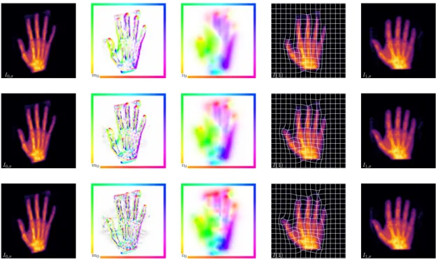
I0,σ mm00 vv00 I(1) I1,σ
I0,σ mm00 vv00 I(1) I1,σ
I0,σ mm00 vv00 I(1) I1,σ
Figure 6.1:Registered hands for regularization parametersβ= 2−1,β= 2−3 and β=
2−5. I
0 is on the left and I1 on the right. In between are the initial momentum, the
initial velocity field and the final imageI(1). The grid onI(1)illustrates the captured deformation of a regular grid onI0. The biggest difference can be seen at the thumb
and the ring finger. With decreasing regularization the thumb inI(1)rotates more to the left to better resemble the pose inI1. The point over the ring finger inI0 does not have
a correspondence inI1. Lower regularization reduces the area covered by the point to
reduce the mismatch term. Note the oscillating Gibbs artifacts in the initial momentum forβ= 2−5. This is caused by the spectral spatial discretization and shows that more
regularization might be needed.
I0,σ mm00 vv00 I(1) I1,σ
Figure 6.2:Registered brains.