EM algorithm coupled with particle filter for maximum
likelihood parameter estimation of stochastic differential
mixed-effects models
Sophie Donnet, Adeline Samson
To cite this version:
Sophie Donnet, Adeline Samson.
EM algorithm coupled with particle filter for maximum
likelihood parameter estimation of stochastic differential mixed-effects models. MAP5 2010-24.
2011.
<
hal-00519576v2
>
HAL Id: hal-00519576
https://hal.archives-ouvertes.fr/hal-00519576v2
Submitted on 21 Jul 2011
HAL
is a multi-disciplinary open access
archive for the deposit and dissemination of
sci-entific research documents, whether they are
pub-lished or not.
The documents may come from
teaching and research institutions in France or
abroad, or from public or private research centers.
L’archive ouverte pluridisciplinaire
HAL
, est
destin´
ee au d´
epˆ
ot et `
a la diffusion de documents
scientifiques de niveau recherche, publi´
es ou non,
´
emanant des ´
etablissements d’enseignement et de
recherche fran¸
cais ou ´
etrangers, des laboratoires
publics ou priv´
es.
EM algorithm coupled with particle
fi
lter for maximum
likelihood parameter estimation of stochastic
differen-tial mixed-effects models
Sophie Donnet
Laboratoire Ceremade, Université Paris Dauphine, France Adeline Samson
UMR CNRS 8145, Laboratoire MAP5, Université Paris Descartes, France
Abstract. Biological processes measured repeatedly among a series of individuals are stan-dardly analyzed by mixed models. These biological processes can be adequately modeled by parametric Stochastic Differential Equations (SDEs). We focus on the parametric maximum likelihood estimation of this mixed-effects model defined by SDE. As the likelihood is not ex-plicit, we propose a stochastic version of the Expectation-Maximization algorithm combined with the Particle Markov Chain Monte Carlo method. When the transition density of the SDE is explicit, we prove the convergence of the SAEM-PMCMC algorithm towards the maximum likelihood estimator. Two simulated examples are considered: an Ornstein-Uhlenbeck pro-cess with two random parameters and a time-inhomogeneous SDE (Gompertz SDE) with a stochastic volatility error model and three random parameters. When the transition density is unknown, we prove the convergence of a different version of the algorithm based on the Euler approximation of the SDE towards the maximum likelihood estimator.
Keywords. Mixed models, Stochastic Differential Equations, SAEM algorithm, Particle Filter, PMCMC, Stochastic volatility, Time-inhomogeneous SDE
1. Introduction
Biological processes are usually measured repeatedly among a collection of individuals or experimental animals. The parametric statistical approach commonly used to discriminate between the inter-subjects variability (the variance of the individual regression parameters) and the residual variability (measurement noise) is the mixed-effects model methodology (Pinheiro and Bates, 2000). The choice of the regression function depends on the context. Dynamical processes are frequently described by deterministic models defined as ordinary differential equations. However, these functions may not capture the exact process, since responses for some individuals may display local "random" fluctuations. These phenomena are not due to error measurements but are induced by an underlying biological process that is still unknown or unexplained today. The perturbation of deterministic models by a random component leads to the class of stochastic differential equations (SDEs). In this paper we develop a parametric estimation method for mixed model defined by an SDE process, called SDE mixed model. Note that SDE mixed models can be viewed as an extension of state space models with random parameters.
Except in the linear case, the likelihood of standard mixed models is intractable in a closed form, making the estimation a hard task. Davidian and Giltinan (1995), Wolfinger (1993),
Pinheiro and Bates (2000) and Kuhn and Lavielle (2005) develop various methods for de-terminitic regression function.
When the regression term is the realization of a diffusion process, the estimation is made more complicated by the difficulties deriving from the SDEs. Parametric estimation of SDE with random parameters (without measurement noise) has been studied by Ditlevsen and De Gaetano (2005), Picchini et al. (2010) or Oravecz et al. (2009) in a Bayesian con-text. SDE mixed model estimation, including measurement noise modeling, is more com-plex and has received little attention. Overgaard et al. (2005) and Tornøe et al. (2005) build estimators based on an extended Kalman filter but without proving the convergence of the algorithm. Donnet and Samson (2008) propose to use a stochastic version of the Expectation-Maximisation algorithm. However, the method involves Markov Chain Monte Carlo (MCMC) samplers which have proved their slow mixing properties in the context of state space models with random parameters.
For state space models with fixed known parameters, the Sequential Monte Carlo (SMC) algorithms have demonstrated their efficiency. However, these techniques are difficult to extent to the case of unknown parameters (Casarin and Marin, 2009). Recently, Andrieu et al. (2010) developed a powerful algorithm combining MCMC and SMC, namely the Particle Markov Chain Monte Carlo (PMCMC), taking the advantage of the strength of its two components. Besides, its convergence toward the exact distribution of interest is established.
To our knowledge, PMCMC methods have been used for parameter estimation only in a Bayesian context and for models without random individual parameters. We propose to focus on maximum likelihood estimation for SDE mixed models by combining a PMCMC algorithm with the SAEM algorithm. When the transition density of the SDE is explicit, we prove the convergence of the SAEM-PMCMC algorithm towards the maximum like-lihood estimator. Two simulated examples are considered, an Ornstein-Uhlenbeck mixed SDE model observed with additive noise and a stochastic volatility mixed model with a time-inhomogeneous SDE, showing the increase in accuracy for the SAEM-PMCMC esti-mates compared with the SAEM-MCMC algorithm (Donnet and Samson, 2008). When the transition density is unknown, we prove the convergence of a different version of the algorithm towards the maximum likelihood estimator.
The paper is organized as follows. In Section 2, we present the SDE mixed model. In Section 3, an estimation method is proposed when the transition density of the SDE is explicit. Section 4 shows numerical results based on simulated data in this case. In Section 5, we extend the approach to general SDEs and prove the convergence of the proposed algorithm. In Section 6 we conclude and discuss the advantages and limitations of our approach.
2. Mixed model defined by stochastic differential equation
2.1. Model and notations
Let y = (yij)1≤i≤n,0≤j≤Ji denote the data, where yij is the noisy measurement of the
observed process for individual i at time tij ≥ ti0, for i = 1, . . . , n, j = 0, . . . , Ji. Let
yi,0:Ji = (yi0, . . . , yiJi)denote the data vector of subject i. We consider that the yij’s are
follows:
yij = g(Xij, εij), εij ∼i.i.d.N(0, σ2), (1)
dXit = a(Xit, t, φi)dt+b(Xit, t, φi, γ)dBit, Xiti0|φi∼π0(·|φi) (2)
φi ∼i.i.d. p(φ;β). (3)
In equation (1),(εij)i,j are i.i.d Gaussian random variables of varianceσ2 representing the
measurement errors andg is the known error model function. The functiong(x, ε) =x+ε
leads to an additive error model. Multiplicative error models or stochastic volatility models can be considered withg(x, ε) =x(1 +ε)org(x, ε) =f(x) exp(ε)with a known functionf.
For each individual i, (Xij)0≤j≤Ji are the values at discrete times(tij)0≤j≤Ji of the
con-tinuous process(Xit)t≥ti0 = (Xit(φi))t≥ti0 defined by equation (2). This process is proper to each individual through the individual parameters φi ∈ Rp involved in the drift and
volatility functionsaandband an individual Brownian motion(Bit)t≥ti0. Functionsaand
b– which may be functions of time, leading to time-inhomogeneous SDEs – are common to thensubjects. They are assumed to be sufficiently regular (with linear growth) to ensure a unique strong solution (Oksendal, 2007). Besides,b depends on an unknown additional volatility parameter γ. The (Bit)and φk are assumed to be mutually independent for all
1≤i, k≤n. The initial conditionXi0 of process(Xit)t≥ti0, conditionally to the individual parameterφiis random with distributionπ0(·|φi). In the following,Xi,0:Ji = (Xi0, . . . , XiJi)
denotes the vector of thei-th process realization at observation times(tij)fori= 1, . . . , n
and X= (X1, . . . , Xn) denotes the whole vector of processes at observation times, for all
individuals. The individual parametersφi are assumed to be distributed with a density
p(φ;β)depending on parameterβ. We denoteΦ= (φ1, . . . , φn)the vector of all individual
parameter vectors.
For simplicity purpose, we restrict to a same number of observations per subject: Ji =J
for alli. The extension to the general case is straightforward.
2.2. Likelihood function
Letθ= (β, γ, σ)be the parameter vector of interest which belongs to some open subsetΘ
of the Euclidean spaceRq with qthe number of unknown parameters. Our objective is to
propose a maximum likelihood estimation ofθ. The likelihood function is well-defined under the assumption of existence of a strong solution to (2). We denotex%→p(x, t−s, s|xs, φi;θ)
the density ofXitgivenφi andXis=xs,s < twith respect to the Lebesgue measure. This
allows us to write the likelihood of model (1-3) as
p(y;θ) = n ! i=1 " p(yi,0:J|Xi,0:J;σ)p(Xi,0:J|φi;γ)p(φi;β)dφidXi,0:J, (4)
where p(y|x;σ), p(x|φ;γ) and p(φ;β) are density functions of the observations given the
diffusion process, the diffusion process given the individual parameters and the individ-ual parameters, respectively. By independence of the measurement errors (εij), we have
p(yi,0:J|Xi,0:J;σ) =#Jj=0p(yij|Xij;σ)wherep(yij|Xij;σ)is the density function associated
to the error model (1). The Markovian property of the diffusion process(Xit)implies
p(Xi,0:J|φi;θ) =π0(Xi0|φi) J
!
j=1
where∆ij =tij−tij−1. Except for a mixed Wiener process with drift and additive noise,
the integral (4) has no-closed form.
Maximizing (4) with respect to θyields the corresponding Maximum Likelihood Estimate
(MLE)θˆof the SDE mixed model (1-3). As the likelihood (4) is not explicit, it has to be
numerically evaluated or maximized. This requires eitheir to know the transition densities explicitely (see Section 3) or to approximate it by an Euler scheme (see Section 5). 3. SDE with explicit transition density: estimation method
In this section, we assume that:
(M0) the SDE defined by (2) has an explicit transition densityp(x, t−s, s|xs, φi;θ).
Even with this assumption, the estimation is complex because thenrandom parametersφi
and random trajectories(Xi,0:J)are unobserved. This statistical problem can be viewed as
an incomplete data model. The observable vectoryis thus considered as part of a so-called complete vector(y,X,Φ).
3.1. Estimation algorithm (SAEM algorithm)
The Expectation-Maximization (EM) algorithm (Dempster et al., 1977) is useful in situa-tions where the direct maximization of the marginal likelihoodθ→p(y;θ)is more complex
than the maximization of the conditional expectation of the complete likelihood
Q(θ|θ$) =E[logp(y,X,Φ;θ)|y;θ$],
wherep(y,X,Φ;θ)is the likelihood of the complete data(y,X,Φ). The EM algorithm is an
iterative procedure: at them-th iteration, given the current valueθ$m−1 of the parameters, the E-step is the evaluation ofQm(θ) =Q(θ|θ$m−1)while the M-step updates$θm−1by max-imizingQm(θ). For cases where the E-step has no closed form, Delyon et al. (1999) propose
the Stochastic Approximation EM algorithm (SAEM) and replace the E-step by a stochas-tic approximation ofQm(θ). The E-step is thus divided into a simulation step (S-step) of
the non-observed data(X(m),Φ(m))with the conditional distributionp(X,Φ
|y;θ$m−1)and a stochastic approximation step (SA-step):
Qm(θ) =Qm−1(θ) +αm
%
logp&y,X(m),Φ(m);θ'−Qm−1(θ) (
,
where(αm)m∈Nis a sequence of positive numbers decreasing to zero.
To fulfill the convergence conditions of the SAEM algorithm (Delyon et al., 1999), we consider the exponential case. More precisely, we assume:
(M1) The parameter space Θ is an open subset included in a compact set of Rq. The
complete likelihoodp(y,X,Φ)belongs to the exponential family i.e.
logp(y,X,Φ;θ) =−ψ(θ) +(S(y,X,Φ), ν(θ)),
where ψand ν are two functions ofθ, S(y,X,Φ)is known as the minimal sufficient statistics of the complete model, taking its value in a subsetS ofRd and
(·,·)is the
In this case, the SA-step of the SAEM algorithm reduces to the approximation ofE[S(y,X,
Φ)|y;θ$]. At step S, a simulation under the conditional distribution p(X,Φ|y;θ$ m−1) is required. However, this distribution is likely to be a complex distribution, resulting in the impossibility of a direct simulation of the non-observed data (X,Φ). Kuhn and Lavielle
(2005) suggest to realize the simulation step via a Markov Chain Monte Carlo (MCMC) scheme, resulting in the SAEM-MCMC algorithm. The S-step consists in constructing a Markov chain with p(X,Φ|y;θ$m−1) as ergodic distribution at the m-th iteration. This S-step by a Markov kernel is detailed in the following subsection.
3.2. Simulation of the latent variables(X,Φ)giveny
We know deal with the construction of a Markov Chain with ergodic distributionp(X,Φ|y;
$
θm−1). First note that conditionally to the observationsy, the individuals are independent. As a consequence, the simulation of each(Xi,0:J, φi)conditionally toy0:Jcan be performed
separately. To ease the reading, in this subsection, we focus on the simulation of the non observed variables(Xi,0:J, φi)of a single individual. Therefore, we omit the index iin the
following. Moreover, we denoteθ= (β, γ, σ)the current values of the parameters and omit
the indexmof the SAEM algorithm iteration.
Standard version of the MCMC alternately simulatesX0:Junder the distributionp(X0:J|y0:J,
φ;γ, σ)and φunder the distribution p(φ|y0:J, X0:J;γ, σ). If the conditional distributions
p(X0:J|y0:J, φ;γ, σ)andp(φ|y0:J, X0:J;γ, σ)cannot be simulated easily, we resort to
Metropo-lis Hastings algorithms for each component ofφand each time component ofX0:J (Donnet
and Samson, 2008). However, standard MCMC algorithms have reached their limits in high dimensional context: they do not exploit the Markovian structure of the data and have proved slow mixing properties. We propose to replace them by the Particle Markov Chain Monte Carlo (PMCMC) algorithm proposed by Andrieu et al. (2010). The idea of the PMCMC algorithm has been first proposed by Beaumont (2003), formalized by Andrieu and Roberts (2009) and developped in the context of state-space models by Andrieu et al. (2010).
Let us consider an ideal Metropolis-Hastings algorithm updating conjointly φ and X0:J
conditionally to y0:J. A new candidate (X0:cJ, φc) would be generated with a proposal
distribution:
q(X0:cJ, φc|X0:J, φ;θ) =q(φc|φ)p(X0:cJ|y0:J, φc;γ, σ).
and accepted with probability:
ρ(X0:cJ, φc|X0:J, φ) = min ) 1,q(φ|φ c) q(φc|φ) p(y0:J|φc;γ, σ)p(φc;β) p(y0:J|φ;γ, σ)p(φ;β) * ,
However, because of the complexity of the model, we are not able to simulate exactly under the conditional distributionp(X0:J|y0:J, φ;γ, σ)and the marginal likelihoodp(y0:J|φ;γ, σ)
has no closed form. These two points can be tackled by an approximation through a particle filter, also called Sequential Monte Carlo (SMC) algorithm. The SMC algorithm produces a set of K particles(X0:(kJ))k=1...K and respective weights(W0:(kJ))k=1...K approximating the
conditional distributionp(X0:J|y0:J, φ; γ, σ)by an empirical measure
ΨK J = K + k=1 W0:(kJ)δX0:(kJ)
Algorithm 1 (SMC algorithm).
• Timej= 0: sampleX0(k)∼π0(·|φ) ∀k= 1, . . . , K and compute the weights:
w0 & X0(k) ' =p&y0, X0(k)|φ;γ, σ ' , W0 & X0(k) ' = w0 & X0(k)' ,K k=1w0 & X0(k)'
• Time j = 1, . . . , J: sample K iid variables X0:!(jk−)1 according to the distribution
ΨK j−1=
,K k=1W
(k)
0:j−1δX0:(kj)−1. Then for eachk= 1, . . . , K, sampleX
(k) j ∼q & ·|yj, X !(k) 0:j−1, φ;γ, σ ' and setX0:(kj)= (X0:!(jk−)1, Xj(k)). Finally compute and normalize the weights:
wj“X0:(kj)”= p“yj, Xj(k)|y0:j−1, X !(k) 0:j−1φ;γ, σ ” q“Xj(k)|yj, X0:!(jk−)1, φ;γ, σ” , Wj(X0:(kj)) = wj“X0:(kj)” PK k=1wj “ X0:(kj)” The simulation of one trajectoryX0:J(called a "run of SMC algorithm" ) under the
approx-imation ofp(X0:J|y0:J, φ;γ, σ)is directly achieved by randomly choosing one particle among
theKparticles with weights(W0:(kJ))k=1...K. Besides, the marginal distributionp(y0:J|φ;γ, σ)
can be estimated through the weights $ pK(y0:J|φ;γ, σ) = 1 K K + k=1 w0 & X0(k) '!J j=1 -1 K K + k=1 wj & X0:(kj) '. . (5)
As a consequence, Andrieu et al. (2010) propose the PMCMC algorithm: Algorithm 2 (PMCMC algorithm).
• Initialization : starting from φ(0), generate X0:J(0) by a run of SMC algorithm –
with K particles– targeting p(X0:J|y0:J, φ(0);γ, σ) and estimate p(y0:J|φ(0);γ, σ) by
$
pK(y
0:J|φ(0);γ, σ)
• At iteration-= 1, . . . , N
(a) Sample a candidateφc
∼q(·|φ(-−1))
(b) By a run of SMC algorithm withKparticles, generateXc
0:Jtargetingp(·|y0:J, φc;γ, σ)
and computep$K(y
0:J|φc;γ, σ)estimatingp(y0:J|φc;γ, σ)
(c) Set (X0:J(-), φ(-)) = (X0:cJ, φc) and p$K(y0:J|φ(-);γ, σ) = $pK(y0:J|φc;γ, σ) with
probability b ρK(X0:cJ, φc|X0:J(%−1), φ(%−1)) = min 1,q(φ(%−1)|φ c) q(φc|φ(%−1)) b pK(y 0:J|φc;γ, σ)p(φc;β) b pK(y 0:J|φ(%−1);γ, σ)p(φ(%−1);β) ff
If the candidate is not accepted, then set(X0:J(-), φ(-)) = (X0:J(-−1), φ(-−1))
andp$K(y
Remark 1. The proposal distributions q(φc
|φ(-)) and q(Xj|yj, Xj−1, φc;γ, σ) used in the SMC algorithm play a crucial role to ensure good mixing properties of the PMCMC algo-rithm. They are discussed with more details for the two simulated examples (Section 4). The most remarkable property of PMCMC is that the distribution of interestp(X0:J, φ|y0:J;
γ, σ)is left invariant by the transition kernel,whatever the number of particles K, the
er-godicity being reached under weak assumptions. More precisely, letΛdenote the auxiliary variables generated by the SMC algorithm, including the set of generated trajectories, the resampling indices and the indice of the particle randomly picked to obtain "a run of SMC algorithm". Andrieu and Roberts (2009) prove thatPMCMC is an exact MCMC algorithm on(X0:J, φ). Under general assumptions, the stationary distribution/πK(Λ, φ)of the
PM-CMC algorithm is such that its marginalized distribution over the auxiliary variablesΛis exactly the distributionp(X0:J, φ|y0:J;γ, σ), independently onK: the PMCMC algorithm
generates a sequence (X0:J(-), φ(-)) whose marginal distribution LK(X0:J(-), φ(-)|y0:J;θ)
is such that for allθ∈Θand for allK >0,
||LK(X
0:J(-), φ(-)|y0:J;θ)−p(X0:J, φ|y0:J;θ)||T V −−−→ !→∞ 0.
where|| · ||T V is the total variation distance (Andrieu et al., 2010).
3.3. SAEM-PMCMC algorithm and convergence
We now combine algorithms PMCMC and SAEM: Algorithm 3 (SAEM-PMCMC algorithm).
• Iteration0: initialization of θ$0 ands0=E %
S(y,X,Φ)|y;θ$0 (
.
• Iterationm= 1, . . . , M:
S-Step: ∗ For each individuali,
· Initialize the PMCMC algorithm by setting φi(0) as the expectation of
p(φ,β$m−1)
· Run N iterations of the PMCMC algorithm with K particles at each iteration, targetingp(Xi,0:J, φi|yi,0:J;$θm−1) ∗ Set X(m)= (X(m) 1,0:J, . . . , X (m) n,0:J)and Φ(m)= (φ (m) 1 , . . . , φ (m) n )the simulated
non observed variables
SA-Step: update ofsm−1 using the stochastic approximation scheme:
sm=sm−1+αm
%
S(y,X(m),Φ(m))−sm−1 (
(6) M-Step: update ofθ$m−1 byθ$m= arg max
θ
(−ψ(θ) +(sm, ν(θ))).
As the PMCMC algorithm can be viewed as a standard MCMC algorithm, the convergence of SAEM-PMCMC can be proved using Kuhn and Lavielle (2005) result. We recall the assumptions of Kuhn and Lavielle (2005).
(M2) The functionsψ(θ)andν(θ)are twice continuously differentiable onΘ.
(M3) The function¯s: Θ−→ S defined ass¯(θ) =0 S(y,X,Φ)p(X,Φ|y;θ)dXdΦ is
contin-uously differentiable onΘ.
(M4) The function-(θ) = logp(y, θ)is continuously differentiable onΘand
∂θ
"
p(y,X,Φ;θ)dXdΦ=
"
∂θp(y,X,Φ;θ)dXdΦ.
(M5) Define L : S ×Θ −→ R as L(s, θ) = −ψ(θ) +(s, ν(θ)). There exists a function
ˆ
θ:S −→Θsuch that
∀θ∈Θ, ∀s∈ S, L(s,θˆ(s))≥L(s, θ).
(SAEM1) The positive decreasing sequence of the stochastic approximation (αm)m≥0 is such that,mαm=∞and,mα2m<∞.
(SAEM2) - : Θ → R and θˆ: S → Θ are d times differentiable, where d is the dimension of S(y,X,Φ).
(SAEM3) For all θ ∈ Θ, 0 ||S(y,X,Φ)||2p(X,Φ
|y;θ)dXdΦ < ∞ and the function Γ(θ) = Covθ(S(X,Φ))is continuous.
(SAEM4) S is a bounded function.
(SAEM5) The transition probabilityΠθof the PMCMC algorithm is Lipschitz inθand generates
a uniformly ergodic chain. The Markov chain(X(m),Φ(m))
m≥0 takes its values in a compact subset.
We comment the different assumptions.
Assumption (M0) is a strong hypothesis, which is partially relaxed in Section 5. Assumptions (M1-M5), (SAEM1-SAEM3) are standard and not restrictive.
Assumption (SAEM4) and the compacity assumption of (SAEM5) are the most restrictive and not really realistic. They could be relaxed using a principle of random boundaries presented in Allassonnière et al. (2009).
Assumption (SAEM5) is verified by the PMCMC algorithm depending on the proposal distributions. Indeed, the Lispchitz property holds if the complete likelihood is continuously derivable which is the case under (M2-M3) and if θ remains in a compact set, which is
realistic in practice. About the uniform ergodicity, Andrieu et al. (2010) prove that if the noise densityp(y|X;σ)is bounded above
sup
y,X
p(y|X;σ)< Mσ, (7)
PMCMC inherits the convergence properties of the corresponding ideal MCMC algorithm. For instance, if q(φc
|φ) = p(φc;β) then the kernel of the ideal MCMC q(Xc
0:J, φc) =
p(φc;β)p(Xc
0:J|y0:J, φc;γ, σ)is independent. For this kernel, the ratiop(Xq(0:XJ0:,φJ|,φy0:)J)is bounded
Theorem1. Assume that (M0-5), (SAEM1-5) hold. Under the assumption that{sm}m≥0 takes its values in a compact subset, the sequence$θmsupplied by the SAEM-PMCMC
algo-rithm converges a.s. towards a (local) maximum of the log-likelihood-(θ) = logp(y;θ).
Remark that despite the SMC approximation in the PMCMC algorithm, the fact that the marginal stationary distribution of MCMC is the exact conditional distributionp(X,Φ|y;θ)
is sufficient to prove the convergence of SAEM-PMCMC. 4. SDE with explicit transition density: simulation study
The respective performances of the SAEM implemented with a standard MCMC and of the SAEM combined with the PMCMC are compared to two models of various complexity: the Ornstein-Uhlenbeck process and the time-inhomogeneous Gompertz process.
In order to validate our results, we perform a large scale simulation study with various sets of parameters and designs (n, J). Moreover, we study the influence of the number of
particles and of the proposals involved the SMC algorithm.
We compare the results using a biais and RMSE criteria. More precisely, for each condition (parameters, design, number of iterations) 100 datasets are generated. The corresponding estimate is obtained on each data set using both the SAEM-PMCMC algorithm and the SAEM-MCMC algorithm. Letθ$rdenote the estimate ofθ obtained on ther-th simulated
dataset, forr= 1, . . . ,100by the corresponding algorithm. The relative bias 1001 ,r($θr−
θ)/θand relative root mean square error (RMSE)
1 1 100
,
r(θ$r−θ)2/θ2for each component
ofθare computed for both algorithms.
The SAEM algorithm requires initial value θ0 and the choice of the sequence (αm)m≥0.
The initial values are chosen arbitrarily as the convergence of the SAEM algorithm little depends on the initialization. The step of the stochastic approximation scheme is chosen as recommended by Kuhn and Lavielle (2005):αm= 1during the first iterations1≤m≤M1,
and αm = (m−M11)0.8 during the subsequent ones. Indeed, the initial guess θ0 might be far from the maximum likelihood value and the first iterations with αm = 1 allow the
sequence of estimates to converge to a neighborhood of the maximum likelihood estimate. Subsequently, smaller step sizes during M −M1 additional iterations ensure the almost sure convergence of the algorithm to the maximum likelihood estimate. We implement the SAEM algorithm withM1= 60andM = 100iterations.
4.1. Example 1: Ornstein-Uhlenbeck process
4.1.1. Ornstein-Uhlenbeck mixed model
The Ornstein-Uhlenbeck process has been widely used in neuronal modeling, biology, and finance (seee.g.Kloeden and Platen, 1992). Consider an SDE mixed model driven by the Ornstein-Uhlenbeck process and an additive error model
yij = Xij+εij, εij∼ N(0, σ2), dXit = − 2 Xit τi − κi 3 dt+γdBit, X0= 0
whereκi∈R,τi >0. We setφi= (log(τi), κi)the vector of individual random parameters.
θ = (logτ, κ, ωτ, ωκ, γ, σ). This model can be easily discretized, resulting in a state-space
model with random individual parameters:
yij = Xij+εij, εij ∼ N(0, σ2),
Xij = Xiji−1e−∆ijτi−κiτi(1−e−∆ijτi) +ηij,
ηij ∼ N40, γ2τi(1−e−∆ijτi)5.
The vectorXi = (xi1, . . . , xiJ) conditional on φi is Gaussian with mean vector miX and
covariance matrixGiX equal to
miX =
&
τiκi
&
1−e−tiτi1', . . . , τiκi&1−e−tiJτi ''$,
GiX = 2 τiγ2 2 2 1−e−
2 min(tij ,tik)
τi
3
e−|tijτi−tik|
3 1≤j,k≤J
, (8)
where$is the transposed vector. Altough this SDE is linear, the Gaussian transition density
p(Xij,∆ij, tij−1|Xij−1, φi;θ)is a nonlinear function ofφi. Thus, the likelihood has no closed
form and the exact estimator ofθis unavailable.
This example is a toy example. First, we compare the performances of the SAEM algo-rithm implemented with a simple MCMC to those of the SAEM-PMCMC algoalgo-rithm. Next, we compare the influence of the number of particles K and the choice of the proposal
distributionq(Xtij|Xij−1, yij, φi;θ)in the SAEM-PMCMC.
4.1.2. Simulation step of the SAEM algorithm
Whereas the conditional distributionp(Xi,1:J|, yi,0:J, φi;θ)is Gaussian, the joint distribution
p(Xi,1:J, φi|, yi,0:J, φi;θ)is not explicitly and we have to resort to a approximate simulation
at the S-step.
A first solution is to implement a standard MCMC algorithm, alternatively simulating under the distributions p(Xi,1:J|, yi,0:J, φi;θ) and p(φi|, yi,0:J, Xi,1:J;θ) for each subject.
The posterior distributionp(Xi,1:J|, yi,0:J, φi;θ) is Gaussian with easily computable mean
vector and variance matrix derived from (8). Similarly, the posterior distribution ofκi is
Gaussian with explicit mean and variance. On the other hand, the posterior distribution of
τi is not explicit and we use a Metropolis-Hastings step with a random walk proposal.
If we consider implementing a PMCMC kernel at the S-step, we have to choose two pro-posalsq(Xtij| Xij−1, yij, φi;θ)and q(·|φi). In this particular linear example, the proposal
q(Xij|Xij−1, yij, φi;θ)can be the optimal proposal, the exact posterior densityp(Xij|Xij−1,
yij, φi;θ), which minimizes the variance of the particle weights. Indeed, this distribution
is explicit for the Ornstein-Uhlenbeck, Gaussian with conditional mean and variance easily computable.
As an alternative, we also consider the transition density p(Xij|Xij−1, φi;θ) as proposal.
The proposal q(·|φ) for the individual parameters φ within the PMCMC algorithm is a classical random walk on each component of vectorφ.
4.1.3. Maximization step of the SAEM algorithm
The SAEM algorithm is based on the computation of the sufficient statistics for the maxi-mization step. The statistics for the parametersµ= (logτ, κ),Ω =diag(ω2
the three classic ones for mixed models (seee.g.Samson et al., 2007): S1(y, X,Φ) = n + i=1 φi, S2(y, X,Φ) = n + i=1 φiφ$i, S3(y, X,Φ) = n + i=1 (yi−Xi)$(yi−Xi).
Let s1m, s2m, s3m denote the corresponding stochastic approximated conditional
expecta-tions at iterationmof SAEM. The M step for these parameters reduces to
$ µ(m)= 1 ns1m Ω$ (m)= 1 ns2m− 1 n2s1ms$1m σ$(m)= 6 1 ns3m
The sufficient statistic corresponding to the parameter γ depends on the SDE. For the
Ornstein-Uhlenbeck, we have S4(y, X,Φ) = n + i=1 J + j=1 & Xitiij−X i itij−1e− ∆ijτi −κiτi(1−e−∆ijτi) '2 .
The M step is thus$γ(m)=1nJ1 s4m.
Convergence assumptions (M0-5), (SAEM1-2) are easily checked on this example. (SAEM3) is implied by (SAEM4). (SAEM4) is not theoretically verified even if in practice, this is not a problem. Finally, given our choice of proposals for PMCMC, (SAEM5) also holds, the compacity being verified in practice.
4.1.4. Simulation design and results
Two different designs are used for the simulations with equally spaced observation times:
n= 20,J = 40,∆ =0.5and n= 40,J = 20,∆ = 1, t0= 0. Two sets of parameter values are used. The first set is log(τ) = 0.6, κ= 1, ωτ = 0.1, ωκ = 0.1, γ = 0.05, σ = 0.05.
The second set uses greater variances and is log(τ) = log(10), κ= 1, ωτ = 0.1,ωκ = 0.1,
γ= 1,σ= 1. For each design and each set of parameter values, one hundred datasets are simulated.
The SAEM-PMCMC and SAEM-MCMC algorithms are initialized. For the first set of parameters, we setlog(!τ)0= 1.1,κ$0= 1.5,ω7τ0= 0.5,ω7κ0 = 0.5,$γ0= 0.25andσ$0= 0.25, i.e. the initial standard deviations are 5 times greater than the true standard deviations. For the second set of parameters, we set log(!τ)0 = log(10) + 0.5, $κ0 = 1.5, ω7τ0 = 0.5, 7
ωκ0= 0.5,$γ0= 5andσ$0= 5. The SAEM-MCMC algorithm is implemented withN= 100 MCMC iterations. Several values ofN andKare used in the SAEM-PMCMC algorithm.
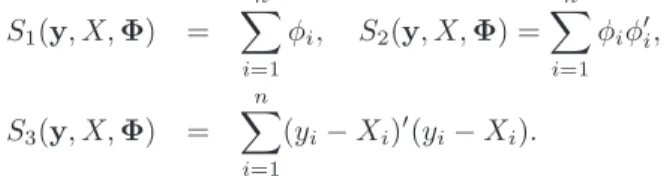
Figure 1 presents the convergence of the SAEM-PMCMC algorithm for one dataset sim-ulated with the second set of parameters, n = 40 and J = 20. This illustrates the low
dependence of the initialization of SAEM and the quick convergence in a small neighbor-hood of the maximum likelineighbor-hood.
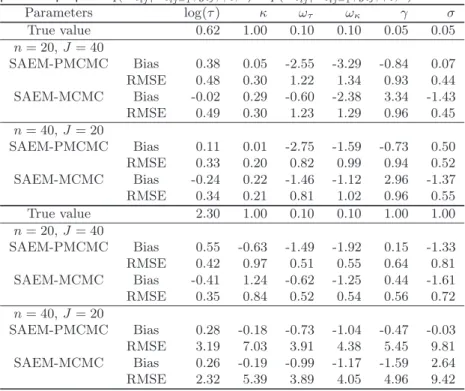
Table 1 presents the bias and RMSE (%) of the SAEM-PMCMC and SAEM-MCMC al-gorithms obtained for the two designs and two sets of parameters. The results are almost identical for both algorithms and very satisfactory (bias less than 3% and RMSE less than
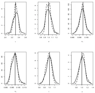
Figure 1.Convergence of the SAEM-PMCMC estimateslog(!τ)m,bκm,ωcτ m,ωcκm,γmb andσmb along the SAEM iterations for one dataset simulated with the Ornstein-Uhlenbeck mixed model, with the second set of parameters,n= 40andJ= 20. Horizontal lines represent the true values.
10%). Figure 2 shows the density of the estimators obtained by both algorithms with
n = 40, J = 20 and the second set of parameters. The SAEM-PMCMC algorithm has
slightly greater bias than SAEM-MCMC for the standard deviations of the random effects (ωτ andωκ). On the contrary, the bias forγ andσare always lower with SAEM-PMCMC
than with SAEM-MCMC.
In this particular linear model, the standard MCMC on (X,Φ) is "ideal" as the distribution p(Xi,0:J|yi,0:J, φi)can be sampled exactly. As a consequence, the SAEM-PMCMC can not
be hopped to perform better. However, results show that the use of a particle approximation ofp(Xi,0:J|yi,0:J, φi)does not deteriorate the quality of estimation.
Besides, note that the design (n, J) of the study affects very little the estimation quality whenγ and σare small (first set of parameters). When γ and σare larger (second set of
parameters), the RMSE are greater with fewer measures per subject (n= 40, J= 20) than
with more (n= 20, J= 40).
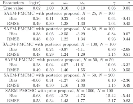
In a second part, we study the influence of the particles number K in the SMC
algo-rithm. Table 2 presents the bias and RMSE obtained on the 100 datasets simulated with the first set of parameters,n = 40, J = 20 and different implementations of the
SAEM-PMCMC algorithm. We successively use K = 25, K = 50 and K = 100 particles and
either N = 50, N = 100 or N = 200 PMCMC iterations, using the exact posterior
dis-tribution q(Xij|Xij−1, yij, φi;θ) = p(Xij|Xij−1, yij, φi;θ). The results are almost
identi-cal. On the contrary, the choice of the proposalq(Xij|yij, Xij−1, φ;γ, σ)in the SMC algo-rithm may affect the result. Table 2 presents results obtained with the transition density
p(Xij|Xij−1, φ;γ, σ)as proposalq. The algorithm fails to converge due to the degeneracy of the particles. We present the results obtained by increasing significantly the number of
par-Table 1. Ornstein-Uhlenbeck mixed model: biais and RMSE (%) for θb ob-tained by the SAEM-PMCMC and SAEM-MCMC algorithms on 100 simulated datasets with two designs (n= 20,J= 40andn= 40,J = 20) and two sets of parameters. PMCMC is implemented withK = 50particles and the exact posterior proposalq(Xtij|Xtij−1, yij, φi;θ) =p(Xtij|Xtij−1, yij, φi;θ).
Parameters log(τ) κ ωτ ωκ γ σ True value 0.62 1.00 0.10 0.10 0.05 0.05 n= 20,J= 40 SAEM-PMCMC Bias 0.38 0.05 -2.55 -3.29 -0.84 0.07 RMSE 0.48 0.30 1.22 1.34 0.93 0.44 SAEM-MCMC Bias -0.02 0.29 -0.60 -2.38 3.34 -1.43 RMSE 0.49 0.30 1.23 1.29 0.96 0.45 n= 40,J= 20 SAEM-PMCMC Bias 0.11 0.01 -2.75 -1.59 -0.73 0.50 RMSE 0.33 0.20 0.82 0.99 0.94 0.52 SAEM-MCMC Bias -0.24 0.22 -1.46 -1.12 2.96 -1.37 RMSE 0.34 0.21 0.81 1.02 0.96 0.55 True value 2.30 1.00 0.10 0.10 1.00 1.00 n= 20,J= 40 SAEM-PMCMC Bias 0.55 -0.63 -1.49 -1.92 0.15 -1.33 RMSE 0.42 0.97 0.51 0.55 0.64 0.81 SAEM-MCMC Bias -0.41 1.24 -0.62 -1.25 0.44 -1.61 RMSE 0.35 0.84 0.52 0.54 0.56 0.72 n= 40,J= 20 SAEM-PMCMC Bias 0.28 -0.18 -0.73 -1.04 -0.47 -0.03 RMSE 3.19 7.03 3.91 4.38 5.45 9.81 SAEM-MCMC Bias 0.26 -0.19 -0.99 -1.17 -1.59 2.64 RMSE 2.32 5.39 3.89 4.05 4.96 9.42
ticles (K= 1000), but we observe the degeneracy of the algorithm on 90% of the simulated
datasets. Morevoer, the bias and RMSE are greater than with the posterior conditional distributionp(Xij|yij, Xij−1, φ;γ, σ).
In conclusion, although the proposalqseems to be crucial in these simulations, the number
of particlesK has less influence on the convergence of the estimation algorithm. This is in
concordance with the theoretical results proved by Andrieu et al. (2010).
However, as emphasized by Andrieu et al. (2010), increasingK can make arbitrarily small
the probability of visiting unfavourable states by the Markov chain, which correspond to large values of the ratio target density to proposal density. But our simulations show that when choosing the "optimal" proposal densityq, namely the exact posterior distribution,
the ratio of the target density to the proposal density seems to have no larges values and thus the number of particlesK has a very low influence. This low influence ofK can also be explained by the fact that the SAEM only requires few iterations of PMCMC, without convergence of the Markov chain to the stationary distribution. The convergence is made over the iterations of SAEM.
Table 2. Ornstein-Uhlenbeck mixed model,n = 20,J = 40: biais and RMSE (%) forθbobtained by the SAEM-PMCMC algorithm on 100 simu-lated datasets. The PMCMC algorithm is successively implemented with posterior proposal q(Xtij|Xtij−1, yij, φi;θ) = p(Xtij|Xtij−1, yij, φi;θ) andK = 25,K= 50orK = 100particles,N = 50,N = 100orN = 200 PMCMC iterations and prior proposal q(Xtij|Xtij−1, yij, φi;θ) = p(Xtij|Xtij−1, φi;θ),K= 1000particles andN = 100iterations.
Parameters log(τ) κ ωτ ωκ γ σ
True value 0.62 1.00 0.10 0.10 0.05 0.05
SAEM-PMCMC with posterior proposal,K= 25,N= 100
Bias 0.26 0.11 0.32 -4.84 0.64 -0.41
RMSE 0.49 0.30 1.28 1.30 1.04 0.45
SAEM-PMCMC with posterior proposal,K= 50,N= 100
Bias 0.38 0.05 -2.55 -3.29 -0.84 0.07
RMSE 0.48 0.30 1.22 1.34 0.93 0.44
SAEM-PMCMC with posterior proposal,K= 100,N= 100
Bias 0.04 0.24 -0.97 -4.11 6.86 -2.68
RMSE 0.48 0.29 1.24 1.29 1.15 0.51
SAEM-PMCMC with posterior proposal,K= 50,N= 50
Bias 0.28 0.04 4.07 -11.61 10.06 -3.32
RMSE 0.49 0.30 1.40 1.55 1.38 0.55
SAEM-PMCMC with posterior proposal,K= 50,N= 200
Bias -0.06 0.31 -1.27 -2.68 6.10 -2.36
RMSE 0.48 0.30 1.16 1.30 1.15 0.49
SAEM-PMCMC with prior proposal,K= 1000,N = 100
Bias -0.63 0.66 -2.78 -4.73 15.42 -5.44
Figure 2.Ornstein-Uhlenbeck mixed model,n= 40,J= 20and second set of parameters. Densi-ties of the estimatorsθbobtained with the SAEM-PMCMC (plain line) and SAEM-MCMC algorithms (dashed line) on 100 simulated datasets, for each component of (logτ, κ, ωτ, ωκ, γ, σ). The true parameter value is the vertical line.
4.2. Example 2: stochastic volatility Gompertz model
4.2.1. Stochastic volatility Gompertz mixed model
The Gompertz model is a well-known growth model (seee.g.Jaffrézic and Foulley, 2006). Recently, Donnet et al. (2010) proposed a stochastic version of this model to take into account random fluctuations in growth process. The stochastic volatility Gompertz mixed model is the following one:
yij = Xij(1 +εij), εij ∼ N(0, σ2),
dXit = BiCie−CitXitdt+γXitdBit, Xi0=Aie−Bi (9)
where Ai >0, Bi >0, Ci >0. We set φi = (logAi,logBi,logCi) the vector of individual
random parameters. The initial conditional is a function of the random individual parame-tersφi. We assume thatlogAi∼i.i.d.N(logA, ωA2),logBi∼i.i.d.N(logB, ωB),logCi∼i.i.d.
N(logC, ω2
C)and the parameter of interest is θ= (logA,logB,logC, ωA, ωB, ωC, γ, σ). By
the Itô formula, the conditional expectation and variance oflog(Xit)|φi, fort≥0, are
E(logXit|φi) = logAi−Bie−Cit−1
2γ2t, Var(logXit|φi) =γ2t.
The transition density of(log(Xt))is explicit, Gaussian and equals to
logp(logXij,∆ij, tij−1|logXij−1, φi;θ) =−12log(2πγ2∆ij)
−1 2
(logXij−logXij−1+Bie−Ctij−1(e−Ci∆ij−1)−12γ2∆ij)2
which is a nonlinear function ofφi. As a consequence, the likelihood has no closed form
and the exact estimator ofθ is unavailable.
4.2.2. Simulation step of the SAEM algorithm
First, the S step of the SAEM algorithm is tackled with a standard MCMC algorithm. Due to the multiplicative structure of the observation noise, the distributionp(Xi,0:J|yi,0:J, φi, θ)
is no more explicit and we have to resort to a random walk proposal to simulate the trajec-toriesXi,0:Jconditionally to the observationsyi,0:J. The components ofXi,0:J are updated
time by time using a random walk proposal. A random walk proposal is also used to simulate the individual parametersφi from the conditional distribution.
Secondly, we implement the SAEM-PMCMC algorithm and the proposalq(Xij|Xij−1, yij,
φi;θ)has to be chosen. We propose to approximate the ideal proposalp(Xij|Xij−1, yij, φi;θ)
by a Gaussian distribution with mean and variance deduced from the true ones. More precisely, we consider the following proposal onlogXtij
q(logXtij|logXij−1, yij, φi;θ) =N(mXij,post,ΓXij,post),
with ΓXij,post = 4 σ−2+ (γ2∆ ij)−15− 1 , mXij,post = ΓXij,postµXij,post,
µXij,post = 2logy ij σ2 + 1 γ2∆ ij 2 logXij−1−Bie−Citij−1(e−Ci∆ij −1)− γ2∆ ij 2 33 .
and then take the exponential to obtain a candidate forXtij. The proposalq(·|φ)for the
individual parametersφwithin the PMCMC algorithms is a classical random walk on each
component of the vectorφ.
4.2.3. Maximization step of the SAEM algorithm
Within the SAEM algorithm, for parametersµ= (logA,logB,logC),Ω =diag(ω2
A, ω2B, ωC2)
and σ, the sufficient statistics and the M step are the same as in Example 1. As the
pa-rameterγ appears both in the expectation and the variance of log(Xt)|φ, its estimator is
not the same as in Example 1. The sufficient statistic corresponding toγis
S4(y,logX,Φ) = n + i=1 J + i=1 ∆ij4logXitij−logXitij−1+Bie−Citij−1(e−Ci∆ij −1)5 2 .
Lets4mdenote the stochastic approximation of this sufficient statistic at iterationmof the
SAEM algorithm. For the sake of simplicity, we assume that the step size∆ij is a constant
∆. The estimator$γmat iterationmis deduced by maximizing the complete likelihood:
$ γm= 8 2 ∆ 2 −1 + 6 1 + s4m nJ 3
Table 3. Stochastic volatility Gompertz mixed model: bias and RMSE (%) of bθobtained by the SAEM-PMCMC and SAEM-MCMC algorithms, on the 100 datasets with two designs (n = 20, J= 40andn= 40,J= 20) and two sets of parameters.
Parameters logA logB logC ωA ωB ωC γ σ
True value 8.01 1.61 2.64 0.10 0.10 0.10 0.40 0.22 n= 20,J= 40 SAEM-PMCMC Bias 0.01 -0.07 0.03 -0.69 -2.31 -1.79 2.77 -0.04 RMSE 0.61 1.16 0.91 2.90 9.71 5.98 11.15 3.15 SAEM-MCMC Bias 2.04 1.713 -1.99 -8.00 -5.00 -7.55 61.93 -2.56 RMSE 2.16 2.07 2.19 8.15 10.87 9.14 63.78 4.30 n= 40,J= 20 SAEM-PMCMC Bias 0.05 -0.30 0.12 -1.92 -2.38 -1.41 6.79 -0.81 RMSE 0.797 1.64 1.36 4.53 14.88 9.10 18.54 3.31 SAEM-MCMC Bias 2.37 1.90 -1.98 -6.76 -4.58 -8.17 77.66 -2.00 RMSE 2.52 2.43 2.33 7.20 14.80 10.73 79.74 4.01 True value 8.01 1.61 2.64 0.10 0.10 0.10 0.80 0.26 n= 20,J= 40 SAEM-PMCMC Bias 0.56 0.72 -0.44 -1.11 -6.56 -1.97 1.67 -0.15 RMSE 1.47 1.90 1.67 3.90 13.10 6.33 11.20 3.20 SAEM-MCMC Bias 4.76 4.64 -3.67 -7.58 -11.92 -11.49 62.90 -2.60 RMSE 4.92 4.95 4.01 7.83 16.55 12.08 75.11 4.84 n= 40,J= 20 SAEM-PMCMC Bias 0.36 0.38 -0.47 -0.70 -2.16 -1.31 0.37 0.82 RMSE 1.07 1.41 1.43 2.21 8.84 4.64 9.55 3.57 SAEM-MCMC Biais 4.37 4.11 -3.60 -8.15 -8.05 -10.05 49.70 -4.33 RMSE 4.46 4.31 3.81 8.26 11.38 10.55 52.36 5.64 4.2.4. Simulation results
We propose to simulate two experimental designs with the same observation times for all individuals: n= 20, J = 40,∆ = 0.01 andn= 40, J = 20,∆ = 0.02(t0= 0), respectively. As in Donnet et al. (2010), we use the following population parameters: logA= log(3000),
logB = log(5), logC = log(14), ωA = 0.1, ωB = 0.1, ωC = 0.1. Two levels of variability
γ and σ are taken respectively equal to 40.4,1/√205 and40.8,1/√155 and referred to as
first and second set of parameters thereafter. For each design and each set of parameters,
100datasets are simulated and θ is estimated with the two algorithms (SAEM-PMCMC
and SAEM-MCMC). The SAEM algorithm is initialized withlog"A0= 8.21,log"B0= 1.81,
"
logC0 = 2.84, ω7A0 = 0.5, ω7B0 = 0.5, ω7C0 = 0.5, $γ0 = 1.2, σ$0 = 0.66. The PMCMC is implemented withN = 100 iterations andK = 50particles. The MCMC is implemented withN= 100 iterations.
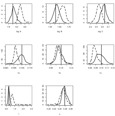
Bias and RMSE (%) are presented in Table 3. Both algorithms give satisfactory results overall (bias and RSME≤20%except forγ). Nevertheless, we clearly see that the
SAEM-PMCMC algorithm performs better than the SAEM-MCMC algorithm. Indeed, for the population means(logA,logB,logC), the population standard deviations(ωA, ωB, ωC)and
σ, the bias and RMSE are smaller for SAEM-PMCMC even if SAEM-MCMC results are already small. The difference is obvious for γ, which is estimated with a large bias by SAEM-MCMC (up to a bias of77%) while this is not the case for SAEM-PMCMC (bias < 7%). This phenomenon is accentuated when the variabilitiesγ and σ increase (second
Figure 3. Stochastic volatility Gompertz mixed model, n = 20, J = 40 and second set of parameters. Densities of the estimators θb obtained with the SAEM-PMCMC (plain line) and SAEM-MCMC algorithms (dashed line) on 100 simulated datasets, for each component of
(logA,logB,logC, ωA, ωB, ωC, γ, σ). The true parameter value is th vertical line.
also be observed in Figure 3 where we plot the densities of the parametersθ$among the100 simulated datasets for the second set of parameters withn= 20andJ = 40.
The improved quality of estimation has a computational cost since it takes less than 8
minutes for the SAEM-MCMC and nearly 23 minutes for the SAEM-PMCMC algorithm to supply results. However, estimating precisely the population parameters is a key issue in population studies (such a genetic specification) and a bias can have real consequences on the conclusions.
5. Theoretical results for general SDE requiring Euler approximation
The class of SDEs considered under assumption (M0) is limited. For a general SDE, we propose to approach the process by an Euler-Maruyama scheme, leading to an approximate model with an explicit (Gaussian) transition density.
5.1. Euler approximation
For the sake of simplicity, we now consider that∀i= 1. . . n,∀j= 0. . . J,tij =jand that the
interval time[tj, tj+1[, we define an approximate diffusion by the recursive Euler-Maruyama scheme of step size1/r by : Xi0(r)∼π0(·|φi)and
Xij(0) = Xij−1(r), Xij(u+ 1) = Xij(u) + 1 r a(Xij(u), tj−1+u/r, φi) (10) + 6 1 r b(Xij(u), tj−1+u/r, φi, γ)Uu
where the variablesUu are iid unit centered Gaussian. Then Xij(r) is a realization of the
approximate diffusion at timetj. We consider the error model
yij=g(Xij(r), εij) (11)
Equations (10), (11) and (3) define the so-called approximate mixed model. Under this model, the likelihood of the observationsyis :
p(r)(y;θ) = n ! i=1 " p(yi,0:J|Xi,0:J(r);σ)p(r)(Xi,0:J(r)|φi;γ)p(φi;β)dφidXi,0:J(r),
wherep(r)(Xi,0:J(r)|φi;θ)is the density of the Euler approximationXij(r)givenφi.
5.2. SAEM-PMCMC on the approximate Euler model
A first approach to estimateθis to use the algorithm SAEM-PMCMC presented in Section
3 on the approximate model. In that case, Theorem 1 implies the following corollary: Corollary 1. Assume that (M1-5), (SAEM1-5) hold for the approximate model. Under the assumption that{sm}m≥0 takes its values in a compact subset, the sequence{θ$m}m≥0 generated by the algorithm SAEM-PMCMC on the approximate Euler model converges to a (local) maximum of the likelihoodp(r)(y;θ)of the approximate model.
The main limit of this result is that the SAEM-PMCMC converges to the maximum of the Euler approximate likelihoodp(r)(y;θ)instead of the maximum of the exact likelihood
p(y;θ). Donnet and Samson (2008) prove that there exists a constantCsuch that the total
variation distance betweenp(r)(y;θ)and the exact likelihoodp(y;θ)can be bounded by
||p(r)(y;θ)−p(y;θ)||T V ≤C
r
This results says that the two likelihoods are close but this does not imply that the two maxima are close.
A solution would be to considerr→ ∞, so that the Euler approximation converges to the exact diffusion. This requiresrto increase along the iterations of the SAEM algorithm, also
implying the Euler approximate model and the likelihood to change with the iterations. The concept of stationary distribution of PMCMC is no more valid in this context. We could imagine a reversible jump approach for the simulation step of the SAEM algorithm. But even in this case, as the approximate likelihood changes with the iterations, it is not possible to prove the convergence of the SAEM algorithm.
From a practical point of view, the choice of r is sensitive because it adds intermediate latent variables to the model. A large value of r is prefered as the Euler approximate likelihood is closer to the exact likelihood. However, it is well known that a large volume of latent variables is difficult to handle within a MCMC or PMCMC approach. This has been discussed by Roberts and Stramer (2001) in a general diffusion context and by Donnet and Samson (2008) for SDE mixed models. Furthermore, as emphasized by Roberts and Stramer (2001), when r → ∞, MCMC algorithms with r additional latent variables are
unable to correctly estimate γ. Indeed, in that case, the density p(r)(xj|xj−1, φ;γ)of the Euler approximate diffusion converges to the likelihood of the continuous path(Xt)t∈[tj−1,tj]
given by the Girsanov formula. It is well-known that it is not possible to estimate the volatility from this continuous path likelihood.
5.3. Exact theoretical convergence for a SAEM algorithm coupled with a SMC algorithm
To circumvent the problem of the estimation ofγ, we restrict to the estimation of
θ= (β, σ)
withγ assumed to be known. To estimateθ, we propose a theoretical algorithm coupling
SAEM with a naive SMC. This algorithm is known to have bad numerical properties (this is the reason why we do not implement it) but we prove that it supplies a sequence(θ$m)m∈N
converging a.s. towards a local maximum of theexact likelihoodlogp(y;θ). This theoretical
result yields to a consequent improvement of Corollary 1.
Now, we present the SMC that we propose to use in the simulation step of the SAEM algorithm. In the literature, SMC algorithms have originally a filtering purpose to approx-imate the distributionp(X0:J|φ, y0:J;θ). However, they have been rapidly extended to the
case where the parametersφ are also sampled. In the following, we present a naive SMC
extension targeting the distributionp(r)(X0:J, φ|y0:J;θ)of the approximate model.
Algorithm 4 (Naive SMC algorithm with parameters sampling). • Timej= 0: ∀k= 1, . . . , K, sampleφ0(k)∼p(·;β)andX
(k) 0 ∼π0(·|φ(0k))and compute the weights: W0 & φ(0k), X (k) 0 ' ∝p(r) & y0, X0(k), φ (k) 0 ;θ '
• Timej = 1, . . . , J: sampleK iid variables(φj!(−k)1, X0:!(jk−)1)according to the lawΨK j−1= ,K k=1W (k) 0:j−11φ(jk−1) ,X( k)
0:j−1. Then for eachk= 1, . . . , K, sampleX (k) j ∼q(r) & ·|yj, X !(k) 0:j−1, φ!j(−k1);γ, σ ' and setφ(jk)=φ !(k) j−1andX (k) 0:j = (X !(k) 0:j−1, X (k)
j ). Finally compute and
nor-malize the weights:
Wj & φ(jk), X (k) 0:j ' ∝ p(r) & yj, Xj(k)|y0:j−1, X !(k) 0:j−1φ !(k) j−1;γ, σ ' q(r) & Xj(k)|yj, X !(k) 0:j−1, φ !(k) j−1;γ, σ ' ,
We consider a SAEM algorithm in which the simulation step is performed by this naive SMC sampler. To ensure the convergence of this estimation algorithm towards the exact
maximum likelihood, we need the number of particlesK and the step size1/rof the Euler approximation to vary along the iterations of the SAEM algorithm. Thus Km and rm
denote the number of particles and the step size of the Euler scheme at iteration m of the SAEM algorithm. We denote by(θ$m)m∈N the sequence of estimates supplied by this algorithm. Technical assumptions (E1-4) are required to prove the convergence of the naive SMC sampler and are presented in Appendix.
Theorem2. Assume that there exists a constant c > 1 such that Km varies along the
iterations:
Km=O(log(m)c)
and that rm = min{r ∈ N|r ≥ √Km}. Assume that (M1-5), (SAEM1-4), (E1-4) hold
for the exact model. Then, with probability 1, limm→∞ d($θm,L) = 0 where L = {θ ∈
Θ, ∂θ-(θ) = 0}is the set of stationary points of the exact log-likelihood -(θ) = logp(y;θ).
Theorem 2 is proved in Appendix 7.2. This theoretical result is noteworthy. Indeed, even if the SAEM-SMC algorithm is performed on the approximate Euler model, the algorithm converges to the maximum of the exact likelihood. This is due to the convergence of the Euler approximate SMC towards the exact filter distribution. This powerful result has first been proved by Del Moral et al. (2001). We propose an extension of their results to our SMC (see Lemma 1 in Appendix 7.1). Then, by generalizing the proof of convergence of the SAEM algorithm to an approximate simulation step, we are able to deduce the convergence of the estimates to the maximum of the exact likelihood.
The naive SMC algorithm 4 provides an asymptotically consistent estimate of the target distributionp(r)(X0:J, φ|y0:J;θ)under very weak assumptions but has proved bad properties
in practice (in particular a degeneracy of the parameters due to the resampling step). It can be improved by including a MCMC step on the parametersφ (Doucet et al., 2001).
Although these algorithms remains poorly efficient in practice (explaining the developement of the PMCMC algorithm for instance), they allow to prove this theorem.
6. Discussion
The stochastic differential mixed-effects models are quite widespread in the applied statistics field. However, in the absence of efficient and computationally reasonable estimation meth-ods, a simplifying assumption is often made: either the observation noise or the volatility term are standardly neglected.
In this paper we present an EM algorithm combined with a Particular Monte Carlo Markov Chain method to estimate parameters in stochastic differential mixed-effects models includ-ing observation noise. We prove the convergence of the algorithm towards the maximum likelihood estimator when the transition density is explicit. This proof is classical as the PMCMC acts as an exact marginal MCMC. On the contrary, when we consider SDE with unexplicit transition density, we prove the convergence of the SAEM-PMCMC algorithm to the maximum likelihood of an approximate model obtained by a Euler scheme. We are not able to prove the convergence of this algorithm to the exact maximum likelihood. But we propose the convergence of a SAEM-SMC algorithm to the exact maximum likelihood. The suggested method supplies accurate parameter estimation in a really moderate com-putational time on practical examples. Moreover, it is not restricted to homogeneous time SDE. On various simulated datasets, we illustrate the superiority of this method over the
SAEM algorithm combined with a standard MCMC algorithm. This efficiency is due to the fact that the PMCMC algorithm takes advantage of the Markovian properties of the non-observed process.
A major advantage of this methodology is its automatic implementation. Indeed the gen-eration of the non-observed process does involves less tuning parameters than a standard MCMC, such as the size of the random move in the random walk Metropolis-Hastings algo-rithm. For example, the number of particles is not crucial, as illustrated in Example 1. In this paper we present a PMCMC algorithm where all the particles are re-sampled at each iteration. Many other resampling distributions have been proposed in the literature, trying to achieve an optimal procedure. West (1993) developed an effective method of adaptive importance sampling to address this issue. The procedure developed by Pitt and Shephard (2001) is similar in spirit and has real computational advantages. A stratified resampling is proposed in Kitawaga (1996). Each resampling distribution implies a specific update of the weights.
Acknowledgments
Sophie Donnet has been financially supported by the french program ANR BigMC. References
Allassonnière, S., E. Kuhn, and A. Trouvé (2009). Construction of bayesian deformable mod-els via stochastic approximation algorithm: A convergence study.to appear in Bernoulli.. Andrieu, C., A. Doucet, and R. Holenstein (2010). Particle Markov chain Monte Carlo
methods. J. R. Statist. Soc. B (72), 1–33.
Andrieu, C. and G. O. Roberts (2009). The pseudo-marginal approach for efficient Monte Carlo computations. Ann. Statist. 37(2), 697–725.
Beaumont, M. (2003). Estimation of population growth or decline in genetically monitored populations. Genetics (164), 1139–1160.
Casarin, R. and J.-M. Marin (2009). Online data processing: comparison of Bayesian regularized particle filters. Electron. J. Stat. 3, 239–258.
Davidian, M. and D. Giltinan (1995). Nonlinear models to repeated measurement data. Chapman and Hall.
Del Moral, P., J. Jacod, and P. Protter (2001). The Monte-Carlo method for filtering with discrete-time observations. Probab. Theory Related Fields 120(3), 346–368.
Delyon, B., M. Lavielle, and E. Moulines (1999). Convergence of a stochastic approximation version of the EM algorithm. Ann. Statist. 27, 94–128.
Dempster, A., N. Laird, and D. Rubin (1977). Maximum likelihood from incomplete data via the EM algorithm. Jr. R. Stat. Soc. B 39, 1–38.
Ditlevsen, S. and A. De Gaetano (2005). Stochastic vs. deterministic uptake of dodecane-dioic acid by isolated rat livers. Bull. Math. Biol. 67, 547–561.
Donnet, S., J. Foulley, and A. Samson (2010). Bayesian analysis of growth curves using mixed models defined by stochastic differential equations. Biometrics 66, 733–741. Donnet, S. and A. Samson (2008). Parametric inference for mixed models defined by
stochas-tic differential equations. ESAIM P&S 12, 196–218.
Doucet, A., N. de Freitas, and N. Gordon (2001). An introduction to sequential Monte Carlo methods. InSequential Monte Carlo methods in practice, Stat. Eng. Inf. Sci., pp. 3–14. New York: Springer.
Jaffrézic, F. and J. Foulley (2006). Modelling variances with random effects in non linear mixed models with an example in growth curve analysis. XXIII International Biometric Conference, Montreal, 16-21 juillet.
Kitawaga, G. (1996). Monte carlo filter and smoother for non-gaussian nonlinear state space models. J. Comp. Graph. Statist.(5), 1–25.
Kloeden, P. E. and E. Platen (1992).Numerical solution of stochastic differential equations, Volume 23 ofApplications of Mathematics (New York). Berlin: Springer-Verlag.
Kuhn, E. and M. Lavielle (2005). Maximum likelihood estimation in nonlinear mixed effects models. Comput. Statist. Data Anal. 49, 1020–1038.
Oksendal, B. (2007). Stochastic differential equations: an introduction with applications. Berlin-Heidelberg: Springer-Verlag.
Oravecz, Z., F. Tuerlinckx, and J. Vandekerckhove (2009). A hierarchical Ornstein-Uhlenbeck model for continuous repeated measurement data. Psychometrika (74), 395– 418.
Overgaard, R., N. Jonsson, C. Tornøe, and H. Madsen (2005). Non-linear mixed-effects models with stochastic differential equations: Implementation of an estimation algorithm. J Pharmacokinet. Pharmacodyn. 32(1), 85–107.
Picchini, U., A. De Gaetano, and S. Ditlevsen (2010). Stochastic differential mixed-effects models. Scand. J. Statist. 37, 67–90.
Pinheiro, J. and D. Bates (2000). Mixed-effect models in S and Splus. Springer-Verlag. Pitt, M. and N. Shephard (2001). Auxiliary variable based particle filters. In Sequential
Monte Carlo methods in practice, Stat. Eng. Inf. Sci., pp. 273–293. New York: Springer. Roberts, G. O. and O. Stramer (2001). On inference for partially observed nonlinear
diffu-sion models using the Metropolis-Hastings algorithm.Biometrika 88(3), 603–621. Samson, A., M. Lavielle, and F. Mentré (2007). The SAEM algorithm for group
compar-ison tests in longitudinal data analysis based on non-linear mixed-effects model. Stat. Med. 26(27), 4860–4875.
Tierney, L. (1994). Markov chains for exploring posterior distributions.Ann. Statist. 22(4), 1701–1762.
Tornøe, C., R. Overgaard, H. Agersø, H. Nielsen, H. Madsen, and E. Jonsson (2005). Stochastic differential equations in NONMEM: implementation, application, and com-parison with ordinary differential equations. Pharm. Res. 22(8), 1247–58.
West, M. (1993). Approximating posterior distributions by mixtures. J. Roy. Statist. Soc. Ser. B 55(2), 409–422.
Wolfinger, R. (1993). Laplace’s approximation for nonlinear mixed models. Biometrika 80(4), 791–795.
7. Appendix
7.1. Convergence of the Euler approximate naive SMC
Let us introduce some notations. For any bounded Borel functionf taking real values, we denoteπjθf =E(f(X0:j, φ)|y0:j;θ)the conditional expectation under the exact smoothing
distribution of the exact modelp(X0:j, φ|y0:j;θ)andΨ(J,θK)f =,Kk=1W (k)
0:Jf(φ(k), X
(k) 0:J)the
conditional expectation under the naive SMC distribution of the approximate model with
K particles and a Euler step sizer= min{r∈N|r≥√K}.
Lemma 1. Assume that
E1. The functions a and b are two times differentiable with derivatives w.r.txand φall orders up to 2uniformly bounded w.r.t φ
E2. Θis included in a compact setC. Besides, the functionsθ%→π(φ;β)andσ%→p(y|x;σ)
are continuous onC.
E3. f is a function of (φ, X0:J)taking its values into R, uniformly bounded
E4. There exist κ1 andκ2 independent of σsuch that p(y|x, σ)≤κ1 and such that
p(r) & yj, Xj(k)|y0:j−1, X !(k) 0:j−1φ !(k) j−1;γ, σ ' q&Xj(k)|yj, X !(k) 0:j−1, φ !(k) j−1;γ, σ ' ≤κ2
Then, for anyε >0, for anyj= 1, . . . , J, there exist constantsC1 andC2 independent of
θ such that P&999Ψ(j,θK)f−πj,θf 9 9 9≥δ'≤C1exp 2 −Kδ 2 C2 3
Proof. Following Del Moral et al. (2001) proof, let us define the empirical measureΨ!(K)
j,θ f = ,K k=1W (k) 0:jf(φ !(k)
, X0:!(jk))where X0:!(kj) has been defined in algorithm 4. Set the σ-filed G
generated by the variablesφ(0k), X (k) 0 , . . . , φ (k) j , X (k) 0:j. We have Ψ!(K) j,θ f−Ψ (K) j,θ f = 1 K K + k=1 ηk−E(ηk|G) withηk=f(φ !(k) j , X !(k)
0:j ). By deviation inequalities, under assumption (E3), we obtain that
there exist two constants such that
P(|Ψ!(K) j,θ f −Ψ (K) j,θ f| ≥δ)≤A1exp 2 −KA2δ 2 0f02 3
Next, we introduce the kernelsHj such that : Hjf(φ, X0:j−1) = " p(yj|xj)p(xj|X0:j−1, φ)p(φ)f(φ, X0:j−1, xj)dφdxj Thus we have πjf = πj−1Hjf πj−1Hj1
and the same definitions on the Euler approximate model, with kernelsHK j by
HjKf(φ, X0:j−1) = "
p(yj|xj)p(r)(xj|X0:j−1, φ)p(φ)f(φ, X0:j−1, xj)dφdxj
such thatπK
j f =Er(f(φ, X0:j−1)|y0:j;θ)the conditional expectation under the approximate
model is πKj f = πK j−1HjKf πK j−1HjK1
Then, considering theσ-filed Ggenerated by the variablesφ!0(k), X0!(k), . . . , φj−!(k1), X0:!(kj−)1 we
can write W0:(kj)f−Ψ!jKHjf = 1 K K + k=1 ηk−E(ηk|G) withηk =f(φ(jk), X (k) 0:j) p(r) “ yj,Xj(k)|y0:j−1,X!(0:jk−)1φ!(j−k1);γ,σ” q“Xj(k)|yj,X !(k) 0:j−1,φ !(k) j−1;γ,σ
” . We have to bound|ηk|andE(|ηk|2|G).
Assumption (E4) implies that there exist two constantsC1,C2 such that
|ηk| ≤C1||f||, E(|ηk|2|G)≤C2||f||2 Deviation inequalities imply that there exists a constantC such that
P&999W0:(kj)f−Ψ!K j Hjf 9 9 9≥δ'≤2e−K δ 2 C||f||2
With similar arguments than Del Moral et al. (2001) and assumptions (E1-2), we prove by induction that there exist two constantsA1andA2such that
P(|πjθf−Ψj,θ(K)f| ≥δ)≤A1exp 2 −K δ 2 A20f02 3
where A1 = 3j+2, A2 = C(8ρ)j+1 with C = 2 + 2α and ρ = 2κJ+1/εJ+1, where α is
the constant quantifying the error induced by the Euler scheme and εJ+1 = HJ. . . H11. With regularities assumptions and assumptions (E1-2), we can prove that the constants are independent ofθ.
7.2. Proof of Theorem 2
Proof. At iterationm, the simulation step provides(X(m),Φ(m)) simulated with an ap-proximate distribution Ψ(Km) J,θˆm = ⊗ n i=1Ψ (Km) i,J,θˆm where Ψ (Km)
i,J,θˆm is the empirical measure
ob-tained by the naive SMC for individuali. The stochastic approximation step of the
SAEM-SMC algorithm can be decomposed into:
sm+1 = sm+αm(S(y,X(m),Φ(m))−sm) = sm+αmh(sm) +αmem+αmRm with h(sm) = E(S(y,X,Φ)|y,θˆ(sm))−sm em = S(y,X(m),Φ(m))−Ψ(Km) J,θˆ(sm)S(y,X,Φ) Rm = Ψ(J,Kθˆm(s)m)S(y,X,Φ)−E(S(y,X,Φ)|y,θˆ(sm))
Following Theorem 2 of Delyon et al. (1999) on the convergence of Robbins-Monro scheme, the convergence of SAEM-SMC to the set of stationary points of the exact log-likelihood
-(θ)is ensured if we prove the following assertions:
(a) The functionV(s) =−-(ˆθ(s))is such that for all s∈ S, F(s) =(∂sV(s), h(s)) ≤0
and such that the setV({s, F(s) = 0})is of zero measure.
(b) limm→∞,mk=1αkek exists and is finite with probability 1.
(c) limm→∞Rm= 0 with probability 1.
• To prove assertion 1, we first remark that, asγ is known andθ= (β, σ), we have ∂θlogp(y,X,Φ;θ) = ∂θlogp(r)(y,X,Φ;θ)
∂θlogp(y;θ) = ∂θlogp(r)(y;θ)
Thus under (M1-M5), (SAEM2), the functionsh(s) = ¯s(ˆθ(s))−sandV(s) =−-(ˆθ(s))
verify
(∂sV(s), h(s))=−(∂s-(ˆθ(s)), h(s)) ≤0
With similar arguments than Lemma 2 of Delyon et al. (1999), we can also prove that the setV({s, F(s) = 0})is of zero measure.
• Assertion 2 is proved following Theorem 5 of Delyon et al. (1999). NoteF={Fm}m≥0 the increasing family ofσ-algebra generated by all the random variables used by the SMC algorithm until themth iteration. By construction of the simulation step, the
simulated variables(X(1),Φ(1)), . . . ,(X(m),Φ(m))given θ$
0, . . . ,θ$m are independent.
Consequently, we have that for any positive Borel functionf, E(f(X(m+1),Φ(m+1))|Fm) = Ψ(J,θKm)f
We can then prove that,m
k=1αkek is a martingale, bounded inL2under assumptions (M5) and (SAEM1-4).
• We now prove the almost sure convergence of Rm (assertion 3). The term Rm is
consequence, for the sake of simplicity, we suppose that dequals1. Applying Borel-Cantelli lemma, it is sufficient to prove that,m≥0P(|Rm| ≥3) <∞ for all3 > 0.
We have
Rm= Ψ(J,Kθˆm(s)m)S−πJ,θˆ(sm)S
where πJ,θS =E(S(X,Φ)|y;θ) First, by independence of the individuali = 1. . . n,
we can decomposeS into a sum ofntermsS(X,Φ) =,in=1Si(Xi,0:J, φi). and write:
P&999Ψ(Km) J,θˆ(sm)S−πJ,θˆ(sm)S 9 9 9≥δ'= P-99999 n + i=1 Ψ(K) J,θˆ(sm)Si− n + i=1 E(Si(Xi,0:J, φi)|yi,0:J; ˆθ(sm)) 9 9 9 9 9≥δ . ≤ n + i=1 P2999Ψ(J,Kθˆ)(sm)Si−πi,J,θˆ(sm)Si 9 9 9≥nδ 3
withπi,J,θˆ(sm)Si=E(Si(Xi,0:J, φi)|yi,0:J;θ). Now, we bound each term of the sum by
Lemma 1 and under assumptions (SAEM4), (E1-E2). This implies the almost sure convergence of(Rm)towards 0.