Group-sparse Embeddings in Collective Matrix Factorization
Arto Klami [email protected]
Helsinki Institute for Information Technology HIIT, Department of Information and Computer Science, Univer-sity of Helsinki
Guillaume Bouchard [email protected]
Xerox Research Centre Europe
Abhishek Tripathi [email protected]
Xerox Research Centre India
Abstract
CMF is a technique for simultaneously learn-ing low-rank representations based on a col-lection of matrices with shared entities. A typical example is the joint modeling of user-item, item-property, and user-feature matri-ces in a recommender system. The key idea in CMF is that the embeddings are shared across the matrices, which enables transfer-ring information between them. The existing solutions, however, break down when the in-dividual matrices have low-rank structure not shared with others. In this work we present a novel CMF solution that allows each of the matrices to have a separate low-rank struc-ture that is independent of the other matri-ces, as well as structures that are shared only by a subset of them. We compare MAP and variational Bayesian solutions based on al-ternating optimization algorithms and show that the model automatically infers the na-ture of each factor using group-wise sparsity. Our approach supports in a principled way continuous, binary and count observations and is efficient for sparse matrices involving missing data. We illustrate the solution on a number of examples, focusing in particu-lar on an interesting use-case of augmented multi-view learning.
1. INTRODUCTION
Matrix factorization techniques provide low-rank vec-torial representations by approximating a matrixX∈
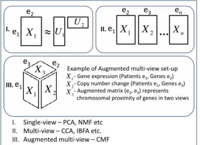
Rn×d as the outer product of two rank-k matrices U1 ∈ Rn×k and U2 ∈ Rd×k (Fig. 1-I). This formu-lation encompasses a multitude of standard data anal-ysis models from PCA and factor analanal-ysis to more
re-e1 e2 e2 e3 1
X
X
2 en…
Xn e1I. Single-view – PCA, NMF etc II. Multi-view – CCA, IBFA etc. III. Augmented multi-view – CMF
I. II. 1
X
X
2 3 X III. e1 e3 e2Example of Augmented multi-view set-up
- Gene expression (Patients e1, Genes e2) - Copy number change (Patients e1, Genes e3) - Augmented matrix (e2, e3) represents chromosomal proximity of genes in two views
1 X 2 X 3 X
U1 2 U 1X
Figure 1. Examples of matrix factorization setups.
cent models such as NMF (Paatero and Tapper, 1994; Lee and Seung, 2001) and various sophisticated fac-torization models proposed for recommender system applications (Mnih and Salakhutdinov, 2007; Koren et al., 2009; Sarwar et al., 2000).
Many data analysis tasks call for more complex se-tups. Multi-view learning (Fig. 1-II) considers scenar-ios with multiple matricesXmthat share the same row
entities but differ in the column entities; for example, X1might contain ratings given ford1 different movies
byndifferent users, whereasX2represents the samen
users withd2 profile features. For such setups the
ap-propriate approach is to factorize the set of matrices
{Xm} simultaneously so that (at least some of) the factors inU1 are shared across the matrices. Models
that share all of the factors are fundamentally equiva-lent to simple factorizations of a concatenated matrix
X = [X1, ...,Xm]. To reach a richer class of models
one needs to allow each matrix to have also private factors, i.e. factors independent of the other matrices (Jia et al., 2010; Virtanen et al., 2012). For the case
of M = 2 the distinction is crystallized by the inter-battery factor analysis (IBFA) formulation of Klami et al. (2013).
Even more general setups with arbitrary collections of matrices that share some sets of entities have been pro-posed several times by different authors, under names such as co-factorization or multi-relational matrix fac-torization, and most end up being either a variant of tensor factorization of knowledge bases (Nickel et al., 2011; Chen et al., 2013) or a special case ofCollective Matrix Factorization(CMF; Singh and Gordon, 2008). In this paper, we concentrate on the CMF model, i.e. on bilinear forms, but the ideas can be easily extended to three-way interactions, i.e. tensors. A prototyp-ical example of CMF, illustrated by Bouchard et al. (2013), would be a recommender system setup where the target matrixX1 is complemented with two other
matrices associating the users and items with their own features. If the users and items are described with the same features, for example by proximities to geograph-ical locations, the setup becomes circular. Another interesting use case for such circular setups is found in augmenting multi-view learning, in scenarios where additional information is provided on relationships be-tween the features of two (or more) views. Figure 1-III depicts an example where the two views X1 and
X2 represent expression and copy number alteration
of the same patients. Classical multi-view solutions to this problem would ignore the fact that the column features for both views correspond to genes. With CMF, however, we can encode this information as a third matrixX3that provides chromosomal promixity
of the probes used for measuring the two views. Even though this kind of setup is very common in practi-cal multi-view learning, the problem of handling such relationships has not attracted much attention. Several solutions for the CMF problem have been pre-sented. Singh and Gordon (2008) provided a maxi-mum likelihood solution, Singh and Gordon (2010) and Yin et al. (2013) used Gibbs sampling to approximate the posterior, and Bouchard et al. (2013) presented a convex formulation of the problem. While all of these earlier solutions to the CMF problem provide mean-ingful factorizations, they share the same problem as the simplest solutions to the multi-view setup; they assume that all of the matrices are directly related to each other and that every factor describes variation in all matrices. Such strong assumptions are unlikely to hold in practical applications, and consequently the methods break down for scenarios where the individ-ual matrices have strong view-specific noise or, more generally, any subset of the matrices has structure in-dependent of the others. In this work we remove the
shortcoming by introducing a novel CMF solution that allows also factors private to arbitrary subsets of the matrices, by adding a group-wise sparsity constraint for the factors.
We use group-wise sparse regularization of factors, where the groups corresponds to all the entities with the same type. In the Bayesian setting, this group-regularization is obtained by using automatic rele-vance determination (ARD) for controlling factor ac-tity (Virtanen et al., 2012). This regularization en-ables us to automatically learn the nature of each fac-tor, resulting in a solution free of tuning parameters. The model supports arbitrary schemas for the collec-tion of matrices, as well as multiple likelihood poten-tials for various types of data (binary, count and con-tinous), using the quadratic lower bounds provided by Seeger and Bouchard (2012) for non-Gaussian likeli-hoods.
To illustrate the flexibility of the CMF setup we dis-cuss interesting modeling tasks in Section 6. We pay particular attention to the augmented multi-view learning setup of Figure 1-III, showing that CMF pro-vides a natural way to improve on standard multi-view learning when the different views lay in related obser-vation spaces. We also show experimentally the key advantage of ARD used for complexity control, com-pared to computationally intensive cross-validation of regularization parameters.
2. COLLECTIVE MATRIX
FACTORIZATION
Given a set ofMmatricesXm= [x
(m)
ij ] describing
rela-tionships betweenEsets of entities (with cardinalities
de), the goal of CMF is to jointly approximate the
ma-trices with low-rank factorizations. We denote by rm
and cm the entity sets corresponding to the rows and
columns, respectively, of them-th matrix. For a simple matrix factorization we have M = 1, E = 2, rm= 1,
andcm= 2 (Fig. 1-I). Multi-view setups, in turn, have E = M + 1, rm = 1 ∀m, and cm ∈ {2, ..., M + 1}
(Fig. 1-II). Some non-trivial CMF setups are depicted in Figures 1-III and 2.
2.1. Model
We approximate each matrix with a rank-K product plus additional row and column bias terms. For linear models, the element corresponding to the row i and columnj of them-th matrix is given by:
x(ijm)= K X k=1 u(rm) ik u (cm) jk +b (m,r) i +b (m,c) j +ε (m) ij , (1)
0 0 0 0 0 0 0 0 0 0 0 0 0 0 1 2 3 4 5 6 T U ? e1 e1 e2 e3 ? ? e4 e5 T X4 1 X X2 e2 ? ? ? ? e3 T X1 T X2 ? ? ? T X3 ? e4 ? X3 ? X4 ? ? ? ? e5 Y 0 0 0 0 0 0 0 0 0 0 0 0 0 0 1 2 3 4 5 6 U k = e1 e2 e3 e4 e5 1 X X2 3 X X4
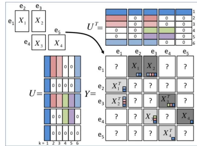
Figure 2.CMF setup encoded as a symmetric matrix
fac-torization, with factors identified by colors. The zero pat-terns in theUmatrix induce private factors in the resulting
Y matrix. Contribution of factors are identified by small
color patches next to the X matrices, and the question
marks (?) represent missing data.
where Ue = [u
(e)
ik] ∈ R
de×K is the low-rank matrix
related to the entity set e, b(im,r) and b(jm,c) are the bias terms for the mth matrix, and ε(ijm) is element-wise independent noise. We immediately see that any two matrices sharing the same entity set use the same low-rank matrix as part of their approximation, which enables sharing information.
The same model can also be expressed in a simpler form by crafting a single large symmetric observation matrixYthat contains allXm, following the
represen-tation introduced by Bouchard et al. (2013). We will use this representation because it allows implementing the private factors via group-wise sparsity. We create one large entity set withd=PE
e=1deentities and then
arrange the observed matrices Xm into Y such that
the blocks not corresponding to any Xm are left
un-observed. The resultingYis of sized×dbut has only (at most)PM
m=1drmdcm unique observed elements. In
particular, the blocks relating the entities of one type to themselves are not observed.
The CMF model can then be formulated as a symmet-ric matrix factorization (see Figure 2)
Y=UUT+ε, (2)
where U ∈ Rd×K is a column-wise concatenation of all of the different Ue matrices, and the bias terms
are dropped for notational simplicity. The noise
ε is now symmetric but still independent over the upper-diagonal elements, and the variance depends on the block the element belongs to. Given this re-formulation, any symmetric matrix factorization tech-nique capable of handling missing data can be used
to solve the CMF problem; the fact that the blocks along the diagonal are unobserved will usually be cru-cial here, since it means that no quadratic terms will be involved in the optimization. In Section 4.2 a vari-ational Bayesian approximation is introduced to learn the model, but before we explain how the basic formu-lation needs to be extended to allow matrix-specific low-rank variations.
3. Group-wise sparse CMF
3.1. Private factors in CMFWithout further restrictions the solutions to (2) tie all matrices to each other; for each factor k the corre-sponding column ofUhas non-zero values for entities in every set e. This is undesirable for many practical CMF applications where the individual matrices are likely to have structured noise independent of other matrices. Since the structured noise cannot be cap-tured by the element-wise independent noise termsε, the model will need to introduce new factors for mod-eling the variation specific to one matrix alone. We use the following property of the basic CMF model: if thek-th columns of the factor matricesUe are null
for all but two entity typesrmandcm, it implies that
the k-th factor impacts only the matrixXm, i.e. the
factor k is a private factor for relation m. To allow the automatic creation of these private factors, we put group-sparse priors on the columns of the matricesUe.
Using the symmetric representation, this approach cre-ates group-sparse factorial representations similar to the one represented in Figure 2. Note that if more than two groups of variables are non-zero for a given factork, it means that it is private for a group of matri-ces rather than a single matrix, and the standard CMF is obtained if no groups equal to zero. In Figure 2 the first factor is a global factor as used in the standard CMF, since it is non-zero everywhere, and the rest are private to some matrices. Note that the last factor rep-resented in light-blue in (k= 6) is interesting because it is a private factor overlapping multiple matrices (X1
andX2) rather than a single one for the other private
factors (matrix X1 for factors 2 and 3, matrixX3 for
factors 4 and 5).
To emphasize the group-wise sparsity structure in im-plementing the private factors, we use the abbreviation gCMF for group-wise sparse CMF i.e. a CMF model with this ability to learn separate private factors. 3.2. Probabilistic model for gCMF
We instantiate the general model by specifying Gaus-sian likelihood and normal-gamma priors for the
pro-jections, so that in (1) we have
ε(ijm)∼ N(0, τm−1), τm∼ G(p0, q0),
u(ike)∼ N(0, α−ek1), αek∼ G(a0, b0).
whereeis the entity set that contains the entityi. The crucial element here is the prior for U. Its purpose is to automatically select for each factor a set of matri-ces for which it is active, which it does by learning large precision αek for factors k that are not needed
for modeling variation for entity set e. In particular, the prior takes care of matrix-specific low-rank struc-ture, by learning factors for whichαekis small for only
two entity sets corresponding to one particular matrix. For the bias terms we use a hierarchical prior
b(im,r)∼ N(µrm, σ2rm), b
(m,c)
j ∼ N(µcm, σ2cm),
µ·m∼ N(0,1), σ2·m∼ U[0,∞].
The hierarchy helps especially in modeling rows (and equivalently columns) with lots of missing data, and in particular provides reasonable values also for rows with no observations (the cold-start problem of new users in recommender systems) throughµrm.
4. LEARNING
4.1. MAP solutionProviding a MAP estimate for the model is straigh-forward, but results in a practical challenge of needing to choose the hyper-parameters{a0, b0, p0, q0}, usually
through cross-validation. This is particularly difficult for setups with several heterogeneous data matrices on arbitrary scales. Then large hyper-priors are needed for preventing overfitting, which in turn makes it dif-ficult to push αek to sufficiently large values to make
the factors private to subsets of the matrices. Hence, we proceed to explain more reasonable variational ap-proximation that avoids these problems.
4.2. Variational Bayesian inference
It has been noticed that Bayesian approaches which take into account the uncertainty about the values of the latent variables lead to increased predictive perfor-mance (Singh and Gordon, 2010). Another important advantage of Bayesian learning is the ability to au-tomatically select regularization parameters by max-imizing the data evidence. While existing Bayesian approaches for CMF used MCMC techniques for ing, we propose here to use variational Bayesian learn-ing (VB) by minimizlearn-ing the KL divergence between a tractable approximation and the true observation
probability. We use a fully factorized approximation similar to what Ilin and Raiko (2010) prsented for Bayesian PCA with missing data, and implement non-Gaussian likelihoods using the quadratic bounds by Seeger and Bouchard (2012). In the following we will summarize the main elements of the algorithm, leaving some of the technical details to these original sources. Gaussian observations For Gaussian data we ap-proximate the posterior with
Q(Θ) = " E Y e=1 K Y k=1 q(αek) de Y i=1 q(u(ike)) !# (3) M Y m=1 q(τm)q(µrm)q(µcm) drm Y i=1 q(b(im,r)) dcm Y j=1 q(b(jm,c)) .
Hereq(α) andq(τ) are Gamma distributions, whereas the others are normal distributions. For all other parameters we use closed-form updates, but ¯Ue, the
mean parameters ofq(Ue), are updated with Newton’s
method for each factor at a time. The gradient-based updates are used because for observation matrices with missing entries closed-form updates would be available only for each element ¯u(ike) separately, which would re-sult in very slow convergence (Ilin and Raiko, 2010). The update rules for Q(Θ) are in the supplementary material.
Non-Gaussian observations For non-Gaussian data we use the approximation schema presented by Seeger and Bouchard (2012), adaptively approximat-ing non-Gaussian likelihoods with spherical-variance Gaussians. This allows an optimization scheme that alternates between two steps: (i) updatingQ(Θ) given pseudo-data Z(which is assumed Gaussian), and (ii) updating the pseudo-dataZby optimizing a quadratic term lower-bounding the desired likelihood potential. The full derivation of the approach is provided by Seeger and Bouchard (2012), but the resulting equa-tions as applied to gCMF are summarized below. We update the pseudodata with
ξm=E[Urm]E[Ucm]
T,
Zm= (ξm−f 0
m(ξm)/κm),
where the updates are element-wise and independent for each matrix. Herefm0 (ξm) is the derivative of the m-th link function−logp(Xm|UrmU
T
cm) andκmis the
maximum value of the second derivative of the same function. Given the pseudo-data Z, the approxima-tion Q(Θ) can be updated as in the Gaussian case, using τm = κm as the precision. Note that the link
functions can be different for different observation ma-trices, which adds support for heterogeneous data; in Section 7 we illustrate binary and count data.
5. RELATED WORK
For M = 1 the model is equivalent to Bayesian (ex-ponential family) PCA. In particular, it reduces to gradient-based optimization for the model by Seeger and Bouchard (2012). For this special case it is typi-cally advisable to use their SVD-based algorithm, since it provides closed-form solution for the Gaussian case. For multi-view setups where every matrix shares the same row-entities the model equals Bayesian inter-battery factor analysis (when M = 2) (Klami et al., 2013) and its extension group-factor analysis (when
M > 2) (Virtanen et al., 2012). However, our
infer-ence solution has a number of advantages. In partic-ular, our solution supports wider range of likelihood potentials and provides efficient inference for missing data. These improvements suggests that the proposed algorithm should be preferred over the earlier solu-tions.
The most closely related methods are the earlier CMF solutions, in particular the ones presented in the prob-abilistic framework. The early solutions by Lippert et al. (2008) and Singh and Gordon (2008) provide only maximum-likelihood solutions, whereas Singh and Gordon (2010) provided fully Bayesian solution by formulating CMF as a hierarchical model. They use normal-Inverse-Wishart priors for the factors, with spherical hyper-prior for the Inverse-Wishart distribu-tion. This implies each factor is assumed to be roughly equally important in describing each of the matrices, and that their model will not provide matrix-specific factors as our model does. For inference they use com-putationally heavy Metropolis-Hastings. Their model also supports arbitrary likelihood potentials and ar-bitrary CMF schemas, though their experiments are limited to cases with M = 2.
6. USE CASES
Even though CMF is widely applicable to factoriza-tion of arbitrary matrix collecfactoriza-tions, it is worth describ-ing some typical setups to illustrate common use cases where data analysis practitioners might find it useful. Augmenting multi-view learning In multi-view learning (Fig. 1-II) the row entities are shared, but the column entities in different views are arbitrary. In many practical applications, however, the column entities share some obvious relationships that are
ig-nored by the multi-view matrix factorization models. A common example considers computing CCA be-tween two different high-throughput systems biology measurements of the same patients, so that both ma-trices are patients times genes (see, e.g., Witten and Tibshirani, 2009). In natural language processing, in turn, we have setups with different languages as row entities and words as column entities (Tripathi et al., 2010). In both cases there are obvious relationships be-tween the column features. In the first example it is an identity relation, whereas in the latter lexigographic or dictionary-based information provides proximity rela-tions for the column entities. Yet another example can be imagined in joint analysis of multiple brain imaging modalities; the column entities correspond to brain re-gions that have spatial relationships even though the level of representation might be very different when, e.g., analyzing fMRI and EEG data jointly (Correa et al., 2010).
Such relationships between the column entities can easily be taken into account with CMF using the cycli-cal relational schema of Figure 1-III. We cycli-call this ap-proach augmented multi-view learning. We can en-code any kind of similarity between the features as long as the resulting matrix can reasonably be mod-eled as low-rank. In the experimental section we will demonstrate setups where the features live in a contin-uous space (genes along the chromosome, pixels in a two-dimensional space) and hence we can measure dis-tances between them. We then convert these disdis-tances into binary promixity relationships, to illustrate that already that is sufficient for augmenting the learning.
Recommender systems The simplest recom-mender systems seek to predict missing entries in a matrix of ratings or binary relevance indicators (Koren et al., 2009). The extensive literature on recommender systems indicates that incorporating additional infor-mation on the entities helps making such predictions (Stern et al., 2009; Fang and Si, 2011). CMF is a natural way of encoding such information, in form of additional matrices between the entities of interest and some features describing them.
While many other techniques can also be used for in-corporating additional information about the entities, the CMF formulation opens up two additional types of extra information not easily implemented by the al-ternative means. The first is a circular setup where both the row and column entities of the matrix of in-terest are described by the same features (Bouchard et al., 2013). This is typically the case for example in social interaction recommenders where both rows and columns correspond to human individuals. The
gCMF−Bernoulli CMF−Bernoulli gCMF−Gaussian 0.7 0.8 0.9 1.0 RMSE CMF−Gaussian M=1 M=5 M=11 0.2 0.4 0.6 0.8 1.0 RMSE MAP
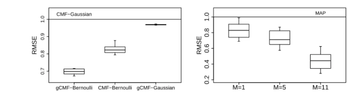
Figure 3.Left: Relative error for a circular setup of M = 5 binary matrices (see text for details), scaled so that CMF
with Gaussian likelihood has error of one. The correct likelihood helps for both gCMF and CMF and modeling the private factors helps for both likelihoods, the combined gain of both aspects being 30%. The results are similar for other values of M >1. Right: Relative error of VB vs MAP, scaled so that zero corresponds to the ground truth and one to the
error of the MAP solution. For small M MAP can still compete (though it is worse than VB already forM = 1), but
for largeM it becomes worthless; forM = 11 VB reduces the error to roughly half. Furthermore, VB requires no tuning
parameters, whereas for the MAP solution we needed to perform cross-validation over two regularization parameters.
other interesting formulation uses higher-order auxil-iary data. For example, the movies in a classical rec-ommender system can be represented by presence of actors, whereas the actors themselves are then repre-sented by some set of features. This leads to a chain of matrices providing more indirect information on the relationships between the entities.
7. EXPERIMENTS
We start with technical validations showing the im-portance of choosing the correct likelihood potential and incorporating private factors in the model, as well as the advantages variational approximation provides over MAP estimation. We then proceed to show how CMF outperforms classical multi-view learning meth-ods in scenarios where we can augment the setup with between-feature relationships.
Since the main goal is to demonstrate the concep-tual importance of solving the CMF task with private factors, we use special cases of gCMF as comparison methods. This helps to show that the difference is re-ally due to the underlying idea instead of the inference procedure; for example, when comparing against Singh and Gordon (2010) the effects could be masked by dif-ferences between Metropolis-Hastings and variational approximation that are here of secondary importance. The closest comparison method, denoted by CMF, is obtained by forcingαek to be a constantαk for every
entity typee. It corresponds to the VB solution of the earlier CMF models and hence does not support pri-vate factors. For the augmented multi-view setup we will also compare against the special cases of gCMF and CMF that use only two matrices over the three entity sets, denoting them by CCA and PCA,
respec-tively. Finally, in one experiment we will also com-pare against gCMF without the bias terms, to illus-trate their importance in recommender systems. For all methods we use sufficiently large K, letting ARD prune out unnecessary components, and run the algo-rithms until the variational lower bound converges. We measure the error by root mean square error (RMSE), relative to one of the methods in each experiment. 7.1. Technical illustration
We start by demonstrating the difference between the proposed model and classical CMF approaches on an artificial data. We sample M binary matrices that form a cycle overM entity sets (of sizes 100−150), so that the first matrix is between the entity sets 1 and 2, the second between the entity sets 2 and 3, and finally the last one is between the M-th and first entity set. We generate datasets that have 5 factors shared by all matrices plus two factors of low-rank noise specific to each matrix. This results in 5 + 2M true factors, and we learn the models with 10+2M factors, letting ARD prune out the extra ones.
Figure 3 (left) shows the accuracy in predicting the missing entries (40% of all) for gCMF as well as a stan-dard CMF model. For both models we show the re-sults for both (incorrect) Gaussian and Bernoulli like-lihoods. The experiment verifies the expected results: Using the correct likelihood improves the accuracy, as does correctly modeling private noise factors.
We use the same setup to illustrate the importance of using variational approximation for inference, this time with Gaussian noise and entity set sizes between 40−80. For MAP we validate the strength of the Gamma hyper-priors forτandαover a grid of 11×11 values for a0 = b0 andp0 =q0, using two-fold
cross-validation within the observed data. In total we hence need to run the MAP variant more than 200 times to get the result, in contrast to the single run of the VB algorithm with vague priors using 10−10 for every
parameter. Figure 3 (right) shows that despite heavy cross-validation the MAP setup is always worse and the gap gets bigger for more complex setups. This illustrates how the VB solution with no tunable hy-perparameters is even more crucial for CMF than it would be for simpler matrix factorizations. For MAP using the same hyper-priors for all matrices neces-sarily becomes a compromise for matrices of different scales, whereas validating separate scales for each ma-trix would be completely infeasible (requiring valida-tion over 2M parameters).
7.2. Augmented multi-view learning
We start with a multi-view setup in computational bi-ology, using data from Pollack et al. (2002) and the setup studied by Klami et al. (2013). The samples are 40 patients with breast cancer, and the two views correspond to high-throughput measurements of ex-pression and copy number alteration for 4287 genes. We compare the models in the task of predicting ran-dom missing entries in both views, as a function of the proportion of missing data.
The multi-view methods use the data as such, whereas the CMF variants also use a thirdd2×d3matrix that
encodes the proximity of the genes in the two views. It is a binary matrix such thatx(3)i,j is one with proba-bility exp(−|li−lj|), whereliis the chromosomal
loca-tion measured in 107 basepairs. This encodes the
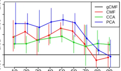
rea-sonable assumption that copy number alterations are more likely to influence the expression of nearby genes. Figure 4 shows how this information helps in making the predictions. For reasonable amounts of missing data, gCMF is consistently the best method, outper-forming both CMF as well as the standard multi-view methods. For extreme cases with at least 80% missing data the advantage is finally lost. The importance of the private factors is seen also in CCA outperforming PCA, whereas CMF and CCA are roughly as accurate; both include one of the strenghts of gCMF.
In another example we model images of faces taken in two alternative lighting conditions, but from the same viewing angle. We observe the raw grayscale pixels values of 50×50 images, and for the CMF methods we use a third matrix (size 2500×2500, of which ran-dom 10% is observed) to encode proximity of pixels in the two views, using Gaussian kernel to provide the probability of one for a binary relation. We train the model so that we have observed 6 images in both views
0.99 1.01 1.03 1.05 10 20 30 40 50 60 70 80 90 Percentage missing RMSE gCMF CMF CCA PCA ● ● ● ● ● ● ● ● ● ● ● ● ● ● ● ● ● ● ● ● ● ● ● ● ● ● ●
Figure 4.Relative prediction error for augmented
multi-view gene experiment, scaled so that gCMF has error one and is represented by the horizontal black line. For reason-able amounts of missing data (x-axis) the methods with pri-vate factors (gCMF and CCA) outperform the ones with-out, and modeling the proximity relationship between the genes (gCMF and CMF) improves the accuracy. The con-fidence intervals correspond to 10% and 90% quantiles over random choices of missing data.
0 10 20 30 40 50 0.70 0.80 0.90 1.00 Neighborhood width RMSE ● ● ● ● ● ● ● ● ● ● ● CMF PCA
Figure 5.Prediction error for a multi-view image
recon-struction task as a function of the neighborhood width in constructing the proximity augmentation view. The aug-mentation helps for a wide range of promixity relationships, and the solution reverts back to the non-augmented accu-racy for very narrow and wide neighborhoods.
and then 7 images for each view alone, for a total of 20 images. The task is to predict the missing views for these images, without any observations.
Figure 5 plots the prediction errors as a function of the neighborhoodσused in constructing the promity rela-tionships. We see that for very narrow and very wide neighborhoods the CMF approach reverts back to the classical multi-view model, since the extra view con-sists almost completely of zeros or ones, respectively. For proper neighborhood relationships the accuracy in predicting the missing view is considerably improved. 7.3. Recommender systems
Next we consider classical recommender systems, us-ing MovieLens and Flickr data as used in earlier CMF experiments by Bouchard et al. (2013). We compare
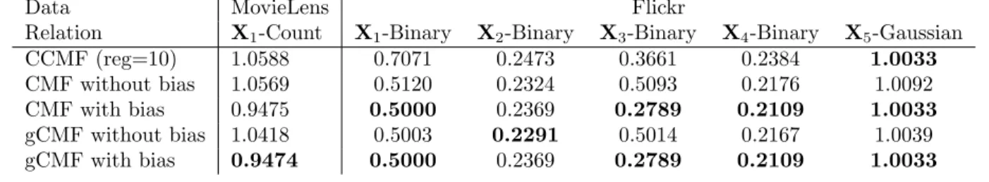
Table 1.RMSE for two recommender system setups, with boldface indicating the best results. The results for convex CMF (CCMF) are taken from Bouchard et al. (2013) for the best regularization parameter values. Our model provides comparable result without the bias terms, without needing any tuning for the parameters, and the bias terms helps considerably with the cold-start problem especially in MovieLens. Without bias terms gCMF also outperforms CMF for all cases, but with the bias terms the methods are practically identical for these data sets. This suggests these data sets do not have strong private structure that could not be modeled with the bias terms alone. It is important to note that allowing for the private factors never hurts; gCMF is always at least as good as CMF.
Data MovieLens Flickr
Relation X1-Count X1-Binary X2-Binary X3-Binary X4-Binary X5-Gaussian
CCMF (reg=10) 1.0588 0.7071 0.2473 0.3661 0.2384 1.0033 CMF without bias 1.0569 0.5120 0.2324 0.5093 0.2176 1.0092 CMF with bias 0.9475 0.5000 0.2369 0.2789 0.2109 1.0033 gCMF without bias 1.0418 0.5003 0.2291 0.5014 0.2167 1.0039 gCMF with bias 0.9474 0.5000 0.2369 0.2789 0.2109 1.0033
gCMF with the convex CMF solution presented in that paper, showing that it finds the same solution when the bias terms are turned off (Table 1). We also illus-trate that modeling the bias terms explicitly is as use-ful for CMF as it has been shown to be for other types of recommender systems. To our knowledge gCMF is the first CMF solution with such bias terms.
Both data sets have roughly 1 million observed entries, and our solutions were computed in a few minutes on a laptop. The total computation time is hence roughly comparable to the times Bouchard et al. (2013) re-ported for CCMF using one choice of regularization pa-rameters. Full CCMF solution is considerably slower since it has to validate over them.
8. DISCUSSION
Collective matrix factorization is a very general tech-nique for revealing low-rank representations for arbi-trary matrix collections. However, the practical ap-plicability of earlier solutions has been limited since they implicitly assume all factors to be relevant for all matrices. Here we presented a general technique for avoiding this problem, by learning the CMF solution as symmetric factorization of a large square matrix while enforcing group-wise sparse factors.
While any algorithm aiming at such sparsity structure will provide shared and private factors for a CMF, the variational Bayesian solution presented in this work has some notable advantages. It is more straighfor-ward than the sampling-based alternative by Singh and Gordon (2010) (which could be modified to in-corporate private factors) while being free of tunable regularization parameters required by the convex so-lution of Bouchard et al. (2013). The model also sub-sumes some earlier models and provides extensions
for them. In particular, it can be used to efficiently learn Bayesian CCA solution for missing data and non-conjugate likelihoods, providing the first efficient Bayesian CCA between binary observations.
One drawback of CMF is its inability to handle multi-ple relations accross two entity type. Tensor factoriza-tion methods alleviate this problem, as illustrated in the recent work on multi-relational data (Glorot et al., 2013; Chen et al., 2013).
Acknowledgments
We acknowledge support from the University Affairs Committee of the Xerox Foundation. AK was also supported by Academy of Finland (grants 251170 and 266969) and Digile SHOK project D2I.
References
Guillaume Bouchard, Shengbo Guo, and Dawei Yin. Convex collective matrix factorization. In Proceed-ings of the 16th International Conference on Artifi-cial Intelligence and Statistics, volume 31 of JMLR W&CP, pages 144–152. JMLR, 2013.
Danqi Chen, Richard Socher, Christopher D. Man-ning, and Andrew Y. Ng. Learning new facts from knowledge bases with neural tensor networks and semantic word vectors. InInternational Conference on Learning Representations, 2013.
Nicolle M. Correa, Tom Eichele, T¨ulay Adali, Yi-Ou Li, and Vince D. Calhoun. Multi-set canonical cor-relation analysis for the fusion of concurrent single trial ERP and functional MRI. Neuroimage, 50(4): 1438–1445, 2010.
Yi Fang and Luo Si. Matrix co-factorization for recom-mendation with rich side information and implicit
feedback. In Proceedings of the 2nd International Workshop on Information Heterogeneity and Fusion in Recommender Systems, pages 65–69. ACM, 2011. Xavier Glorot, Antoine Bordes, Jason Weston, and Yoshua Bengio. A semantic matching energy func-tion for learning with multi-relafunc-tional data. In Inter-national Conference on Learning Representations, volume abs/1301.3485, 2013.
Alexander Ilin and Tapani Raiko. Practical approaches to principal component analysis in the presence of missing data. Journal of Machine Learning Re-search, 11:1957–2000, 2010.
Yangqing Jia, Mathieu Salzmann, and Trevor Darrell. Factorized latent spaces with structured sparsity. In Advances in Neural Information Processing Systems 23, pages 982–990, 2010.
Arto Klami, Seppo Virtanen, and Samuel Kaski. Bayesian canonical correlation analysis. Journal of Machine Learning Research, 14:965–1003, 2013. Yehuda Koren, Robert Bell, and Chris Volinsky.
Ma-trix factorization techniques for recommender sys-tems. Computer, 42(8):30–37, 2009.
Daniel D. Lee and H. Sebastian Seung. Algorithms for non-negative matrix factorization. In Advances in neural information processing systems 13, pages 556–562, 2001.
Christoph Lippert, Stefan-Hagen Weber, Yi Huang, Volker Tresp, Matthias Schubert, and Hans-Peter Kriegel. Relation-prediction in multi-relational do-mains using matrix-factorization. In NIPS Work-shop: Structured Input - Structured Output. 2008. Andriy Mnih and Ruslan Salakhutdinov.
Probabilis-tic matrix factorization. In Advances in neural in-formation processing systems 20, pages 1257–1264, 2007.
Maximilian Nickel, Volker Tresp, and Hans-Peter Kriegel. A three-way model for collective learning on multi-relational data. In ICML, page 809816, 2011. Pentti Paatero and Unto Tapper. Positive matrix fac-torization: A non-negative factor model with op-timal utilization of error estimates of data values. Environmetrics, 5(2):111–126, 1994.
Jonathan R. Pollack, Therese Sorlie, and Charles M. Perou et al. Microarray analysis reveals a major direct role of DNA copy number alteration in the transcriptional program of human breast tumors. Proceedings of the National Academy of Sciences of
the United States of America, 99(20):12963–12968, 2002.
Badrul Sarwar, George Karypis, Joseph Konstan, and John Riedl. Application of dimensionality reduction in recommender system-a case study. Technical re-port, DTIC Document, 2000.
Matthias Seeger and Guillaume Bouchard. Fast vari-ational Bayesian inference for non-conjugate matrix factorization models. In Proceedings of the 15th International Conference on Artificial Intelligence and Statistics, volume 22, pages 1012–1018. JMLR, 2012.
Ajit P. Singh and Geoffrey J. Gordon. Relational learning via collective matrix factorization. In Pro-ceedings of the 14th ACM SIGKDD international conference on Knowledge discovery and data min-ing (KDD), pages 650–658. ACM, New York, NY, USA, 2008.
Ajit P. Singh and Geoffrey J. Gordon. A Bayesian matrix factorization model for relational data. In Uncertainty in Artificial Intelligence, 2010.
David H Stern, Ralf Herbrich, and Thore Graepel. Matchbox: large scale online Bayesian recommenda-tions. InProceedings of the 18th international con-ference on World wide web, pages 111–120. ACM, 2009.
Abhishek Tripathi, Arto Klami, and Sami Virpioja. Bilingual sentence matching using kernel cca. In Ma-chine Learning for Signal Processing (MLSP), 2010 IEEE International Workshop on, pages 130–135. IEEE, 2010.
Seppo Virtanen, Arto Klami, Suleiman A. Khan, and Samuel Kaski. Bayesian group factor analysis. In Proceedings of the 15th International Conference on Artificial Intelligence and Statistics, volume 22 of JMLR W&CP, pages 1269–1277. JMLR, 2012. Daniela M. Witten and Robert J. Tibshirani.
Exten-sions of sparse canonical correlation analysis with applications to genomic data. Statistical applica-tions in genetics and molecular biology, 8(1):1–27, 2009.
Dawei Yin, Shengbo Guo, Boris Chidlovskii, Brian D Davison, Cedric Archambeau, and Guillaume Bouchard. Connecting comments and tags: im-proved modeling of social tagging systems. In Pro-ceedings of the sixth ACM international conference on Web search and data mining, pages 547–556. ACM, 2013.
Supplementary material
This supplementary material for the manuscript “Group-sparse Embeddings in Collective Matrix Fac-torization” provides more details on the variational ap-proximation described in the paper.
Notation
The factors in (3) are
q(u(ike)) =N(¯uik(e),u˜(ike)), q(αek) =G(aek, bek), q(b (m,r) i ) =N(¯b (m,r) i ,˜b (m,r) i ), q(τm) =G(pm, qm), q(b (m,c) j ) =N(¯b (m,c) j ,˜b (m,c) j ).
and we denote by ¯α and ¯τ the expectations of α
and τ. The observed entries in Xm are given by
Om ∈ [0,1]drm×dcm, with nm = Pijo
(m)
ij
indicat-ing their total number. Finally, we denote ˆx(ijm) = x(ijm)−PK k=1u¯ (rm) ik u¯ (cm) jk −¯b (m,r) i −¯b (m,c) j .
Algorithm
The full algorithm repeats the following steps until convergence.
1. For each entity sete, compute the gradient of ¯Ue
using (4) and compute the variance parameter ˜Ue
using (5).
2. Update ¯Ue with under-relaxed Newton’s step.
The element-wise update is ¯u(ike) ← u(ike) +
λ(˜u(ike))−1g(ike) with 0 < λ < 1 as the regulariza-tion parameter.
3. Update the bias terms using (6).
4. Update the automatic relevance determination parameters using (7).
5. For all matricesXmwith Gaussian likelihood,
up-date the noise precision parameters using (8). For all matrices Xm with non-Gaussian likelihood,
update the pseudo-data using (9).
Details
Updates for the factors: The gradient with re-spect to the mean parameters of the factors is com-puted as gik(e)= ¯αeku¯eik+ X m;rm=e ¯ τm X j h −xˆ(ijm)u¯(cm) jk + ¯u (e) iku˜ (cm) jk i (4) X m;cm=e ¯ τm X j h −xˆ(ijm)u¯(rm) ik + ¯u (e) jku˜ (rm) ik i .
For ˜Ue we have closed-form updates
˜ u(ike)= ¯αek+ X m;cm=e ¯ τm X j (¯u(rm) jk ) 2+ ˜u(rm) jk + X m;rm=e ¯ τm X j (¯u(cm) jk ) 2+ ˜u(cm) jk −1 . (5)
Updates for the bias terms: The row bias terms are updated as ˜b(m,r) i = ¯τm X j o(ijm)+σ−2 −1 , (6) ˆb(m,r) i = ˜b (m,r) i τ¯mµi+µrm/σ2rm ,
where µi is a shorthand notation for the mean of x(ijm)−P ku¯ (m) ik u¯ (m) jk −¯b (m,c)
j over the observed entries.
We additionally update q(µrm) using standard
varia-tional update for Gaussian likelihood and prior, and use point estimate for σ2
rm. The updates for the
col-umn bias terms follow naturally.
Updates for the ARD terms: The ARD variance parameters are updated as
aek=aα0 +de/2, (7) bek=b0+ 0.5 ds X i=1 K X k=1 (¯u(ike))2+ ˜u(ike).
Updates for the precision terms: For each ma-trix with Gaussian likelihood the precision is updated as pm=p0+nm/2, (8) qm=q0+ 1 2nm X ij (ˆx(ijm))2+ ˜bi(m,r)+ ˜b(jm,c) + K X k=1 (¯u(rm) ik ) 2u˜(cm) jk + (¯u (cm) jk ) 2u˜(rm) ik + ˜u (cm) jk u˜ (rm) ik # ,
where the sum for qm is over all observed entries.
Updated for the pseudo-data: For each matrix with non-Gaussian data we update the pseudo-data Zmusing
ξm=E[Urm]E[Ucm]
T, (9)
Zm= (ξm−fm0 (ξm)/κm),
where the updates are element-wise and independent for each matrix. Herefm0 (ξm) is the derivative of the
m-th link function−logp(Xm|UrmU
T
cm) andκmis the
maximum value of the second derivative of the same function.
MAP estimation
These update rules can be easily modified to provide the MAP estimate instead; the modifications mostly consist of dropping the variance terms and the re-sulting updates are not repeated here. Similarly, the updates are easy to modify for learning CMF models without private factors, by coercingαek intoαk.