Preprint typeset using LATEX style emulateapj v. 05/12/14
sick, THE SPECTROSCOPIC INFERENCE CRANK
Andrew R. Casey1 Draft version March 11, 2016
ABSTRACT
There exists an inordinate amount of spectral data in both public and private astronomical archives which remain severely under-utilised. The lack of reliable open-source tools for analysing large vol-umes of spectra contributes to this situation, which is poised to worsen as large surveys successively release orders of magnitude more spectra. In thisArticle I introducesick,the spectroscopic inference crank, a flexible and fast Bayesian tool for inferring astrophysical parameters from spectra. sick is agnostic to the wavelength coverage, resolving power, or general data format, allowing any user to easily construct a generative model for their data, regardless of its source. sick can be used to provide a nearest-neighbour estimate of model parameters, a numerically optimised point estimate, or full Markov Chain Monte Carlo sampling of the posterior probability distributions. This generality empowers any astronomer to capitalise on the plethora of published synthetic and observed spectra, and make precise inferences for a host of astrophysical (and nuisance) quantities. Model intensities can be reliably approximated from existing grids of synthetic or observed spectra using linear multi-dimensional interpolation, or aCannon-based model (Ness et al. 2015). Additional phenomena that transform the data (e.g., redshift, rotational broadening, continuum, spectral resolution) are incor-porated as free parameters and can be marginalised away. Outlier pixels (e.g., cosmic rays or poorly modelled regimes) can be treated with a Gaussian mixture model, and a noise model is included to account for systematically underestimated variance. Combining these phenomena into a scalar-justified, quantitative model permits precise inferences with credible uncertainties on noisy data. I describe the common model features, the implementation details, and the default behaviour, which is balanced to be suitable for most astronomical applications. Using a forward model on low-resolution, high S/N spectra of M67 stars reveals atomic diffusion processes on the order of 0.05 dex, previously only measurable with differential analysis techniques in high-resolution spectra. sick is easy to use, well-tested, and freely available online through GitHub under the MIT license.
1. INTRODUCTION
Most of our understanding of astrophysics has been interpreted from spectra. Given how informative spec-troscopic data is to our understanding of astrophysics, it is not surprising that there has been a substantial in-crease of publicly accessible spectra in the last decade. Large scale surveys have driven this trend, each releas-ing in excess of hundreds of thousands (e.g., Drinkwater et al. 2010; Schlegel et al. 2007; Yanny et al. 2009; Stein-metz et al. 2006; Gilmore et al. 2012) of spectra. Millions more spectra are expected in the coming years (e.g., Cui et al. 2012; De Silva et al. 2015).
These spectra are acquired from different astrophysi-cal sources to meet specific scientific objectives. They vary in wavelength coverage, resolution, and noise distri-butions. For these reasons many collaborations expend significant resources to produce bespoke analysis soft-ware for their science program. This usually impedes reproducibility, as many codes still remain closed-source nearly a decade after the original article was published (e.g., Lee et al. 2008), even when the data and results are publicly accessible. As a consequence any comprehensive literature comparison becomes impossible, as systemat-ics are difficult to properly characterise without in-depth knowledge of the methods or access to the software.
In general there are three types of methods employed 1Institute of Astronomy, University of Cambridge,
Mad-ingley Road, Cambdridge, CB3 0HA, United Kingdom; [email protected]
for spectral analysis: measuring the strengths of spec-tral features, pure data-generating models or template-matching methods. Approaches that measure spec-tral features (e.g., equivalent widths; Stetson & Pan-cino 2008) are inexpensive, but regularly encounter prob-lems with blended (often hidden) lines or continuum placement (e.g., see Smiljanic et al. 2014, for a com-parison of techniques). In these instances some sub-jective interaction, tuning, or ad-hoc ‘calibration’ is of-ten invoked (Kordopatis et al. 2013; Sousa et al. 2010). Data-generating methods are computationally expen-sive, repeatedly producing model spectra during run-time (Valenti & Piskunov 1996). Whilst accurate spectra are produced, the known covariances between stellar pa-rameters are routinely ignored, leading to erroneous re-sults (Torres et al. 2012). For template-matching meth-ods (Recio-Blanco et al. 2006; Allende Prieto et al. 2008), synthetic spectra are generated once for a subset of per-mutations of astrophysical quantities, usually discretised across a grid. Although there are differences between these methods, the preparatory steps are usually the same: Spectra are placed at rest-frame by calculating line-of-sight velocities, typically by cross-correlation, be-fore being continuum-normalised to zero and one.
Credible uncertainties can be difficult to discern from these methods. This is because the uncertainties in the Doppler-shift, smoothing, sampling, and normalisation steps are almost always ignored. These effects result in ill-characterised uncertainties in astrophysical
ters. In some cases the uncertainties are simply assumed to be approximately the same for all objects. This is an incorrect approach: there are few, if any, examples of homoscedastic datasets in astrophysics. The noise prop-erties of each spectrum are different, and the parame-ter uncertainties (random and systematic) will differ for every object. Consequently the uncertainties in astro-physical parameters by template-matching methods are generally found to either be incorrectly assumed, under-estimated, or at least ill-characterised.
In addition to affecting the uncertainties, the effects of redshift, continuum normalisation and smoothingwill further bias the reported maximum-likelihood parame-ters. For example, experienced stellar spectroscopists will frequently differ in their decision of continuum place-ment even in the most straightforward cases (e.g., metal-poor stars). There are a number of controversial ex-amples within the literature where the subjective (hu-man) decision of continuum placement have significantly altered the scientific conclusions (e.g., see Kerzendorf et al. 2013, where this issue is discussed in great detail). The implications of these phenomena must be consid-ered if we are to understand subtle astrophysical pro-cesses. Spectroscopy requires open(-sourced) objectivity. One should endeavour to incorporate these phenomena as free parameters into a generative model and infer them simultaneously with the astrophysical parameters.
In thisArticle I present sick: a flexible, well-tested, MIT-licensed probabilistic software package for infer-ring astrophysical (and nuisance) quantities from spec-troscopic data. sick employs approximations to data-generating models. Instead of modelling expensive astro-physical processes (e.g., stars, supernova, and any other interesting astrophysical processes) at run-time, sick approximates the model intensities from pre-computed grids/sets of spectra. Contributory phenomena (e.g., continuum, redshift, rotational broadening, spectral res-olution) are included as free parameters within an ob-jective scalar-justified model. This approach is suitable for a plethora of different astrophysical processes, allow-ing any user to easily construct a generative model usallow-ing existing grids of published spectra, and infer astrophys-ical properties from their data. Aspects of the proba-bilistic model are described in Section 2. The analysis methodology is discussed in Section 3, and a toy model is presented in Section 4. In Section 5 I present a suit-able scientific application that demonstrates the power of forward models with existing data, instead of existing subjective approaches. I conclude in Section 7 with ref-erences to the online documentation and applicability of the software.
2. THE GENERATIVE MODEL
The generative model described below is agnostic as towhat the astrophysical parameters actually describe2.
Typical examples might be properties of supernova (e.g., explosion energies and luminosities), galaxy character-istics from integrated light, or mean plasma properties of a stellar photosphere. There are a plethora of spec-tral libraries (observed and synthetic) published for these types of applications (e.g., Blondin & Tonry 2007; Le 2 However given the research background of the author, these
examples will focus on stellar applications.
Borgne et al. 2004; Husser et al. 2013; Palacios et al. 2010). All of these models are fully-sickcompatible3.
In an ideal world one would avoid spectrum approxi-mations entirely and aim to solve the hydrodynamic and radiative transfer equations to produce accurate model spectra in real-time. This would certainly be a compu-tationally expensive endeavour. It may also be unneces-sary. In practice sick can be sub-classed (by inheriting from theBaseModelclass) to produce more realistic spec-tra at run-time or to allow approximations within exist-ing grids with different approaches. The code is designed to be flexible to suit a range of scientific objectives.
Let us assume that there exists a set of astrophysical parametersθ∗that I wish to infer from some data. I first must produce a spectrum of normalised model intensities (e.g., between 0 and 1) from an existing set (or grid) of spectra. The grid of spectra are expected to span a suit-able range of θ∗ values, but are not required to be reg-ularly spaced inθ∗. Indeed, high-quality observed
spec-tra with irregularly-spaced yet precisely-measured values of θ∗ are perfectly acceptable. There are currently two techniques for producing intensities at any θ∗ value in sick, which are described in the following sections.
2.1. N-Dimensional Linear Interpolation The simplest available method is to linearly interpo-late between the grid of model spectra. The detailed features of most astrophysical model spectra are unlikely to be well-captured by crude linear interpolation in high dimensions. However, theN-dimensional linear interpo-lation scheme is efficient and may be suitable for many astrophysical instances where only a point-estimate ofθ∗ is required.
This approach uses the Quickhull (Barber et al. 1996) algorithm in SciPy (scipy.interpolate.griddataand scipy.interpolate.LinearNDInterpolator; Jones et al. 2001) to interpolate inN-dimensions. The convex hulls required for Quickhull can be globally produced for the entire grid, or for Ngrid local points surrounding
the initial estimate θ∗,estimate (see Section 3.1), where
Ngrid can be specified in the model configuration file.
Quickhull relies on Voronoi tessellation, which produces extremely skewed cells when the grid points {θ∗}grid
vary significantly in magnitude (e.g., as Teff does with
respect to logg in the examples presented here) and will introduce substantial errors in the interpolation. To minimise these effects, sick automatically scales the grid values {θ∗}grid (in both global and local
scenarios) to make δθ∗,dim approximately equal (e.g.,
δTeff,scaled≈δloggscaled).
The model intensitiesIλ,m(θ∗) at wavelengthsλm for
some arbitraryθ∗can be approximated by interpolating
from a ‘nearby’ (local or global) grid{θ∗}grid,
Iλ,m {θ∗}grid;Iλ,m(θ∗), (1)
where, following the nomenclature in parallel work by Czekala et al. (2014), I denote the symbol ;as an in-terpolation operator.
In practice large grids of model spectra are automat-ically cached using efficient memory-mapping, allowing 3 Libraries of published spectra that are ready-to-use are
for the total size of the model grid to far exceed the available random access memory. In other words, grids of model spectra that are hundreds of Gb in size can be efficiently accessed from an external hard disk on any reasonably modern CPU.
2.2. The Cannon
The Cannon (Ness et al. 2015) is a data-driven ap-proach for stellar label determination. The apap-proach makes use of a training set of stars where labels (i.e., θ∗) have been determined with high fidelity. The nor-malised, rest-frame pixel information (on a common bin-ning scale) is then used to build a spectral model for a larger sample of stars. Ness et al. (2015) use observed spectra from APOGEE (Majewski et al. 2010) as their training set, and project spectra from the entire survey to efficiently determine stellar parameters. Here I employ The Cannonas a method for producing model intensities within a grid, using synthetic labels.
For the full description of The Cannon, the reader is directed to Ness et al. (2015). Here I describe the algo-rithm in brief, with a focus on the implementation details in sick. A Cannon model is characterised by a coeffi-cient vector θλ,m that allows for the prediction of the
intensitiyIλ,mfor a given label vectorl, such that at the
i-th model pixel with wavelengthλm,i:
Iλ,m,i=g(λm,i|θλ,m,i) + noise (2)
The vectorθλ,m,iis a set of spectral model coefficients
at eachλm,i. Thus for thei-th pixel there are a number
of coefficientsθλ,m,iand a scatter termsλ,m,i which we
must solve (train). The complexity in θλ,m can be
ad-justed: a linear model is the simplest option, whereas (Ness et al. 2015) employ a quadratic-in-labels model with linear cross-terms. If none is specified, sick will default to a quadratic-in-labels model with linear cross-terms. The label vectorlm (linear vector shown),
lm≡[1, θ∗,i−θ∗,i, θ∗,j−θ∗,j,· · ·] (3)
is generated from a human-readable description of the label vector. Theθ∗offsets are taken as the means of the training set. Before usingThe Cannon, we need to solve for the coefficients{θλ,m, sλ,m}for the label vectorlλ,m
by optimising the log-likelihood function for each λm,i
pixel,
lnp(Iλ,m,i|θ|λ,m,lλ,m,i, s2λ,m,i) =· · · −12[Iλ,m,i−θ | λ,m·lλ,m,i]2 s2 λ,m,i+σθ,2∗,i −12ln(s2 λ,m,i+σ2θ,∗,i) (4)
where σθ∗,i is the intensity uncertainty in the i-th pixel
of the model grid point with parameters θ∗. For the remainder of this Article I will only use synthesised spectra to produce Iλ,m(θ∗), and thus σθ∗,i is zero.
However, this term is included in Equation 4 to demon-strate that The Cannon implementation in sick can be trained from existing observed spectra, as originally utilised by Ness et al. (2015).
2.3. Ancillary Effects
With the model intensities Iλ,m(θ∗) produced, there
are still a number of additional phenomena that must be considered before the model can be reliably compared to the data. I will describe the dominant effects in the con-text of a single observed channel (order/beam/aperture). However, sick allows the user to model any combina-tion of the effects described below, with flexible opcombina-tions for handling multiple channels. For example, although redshiftz is an astrophysical phenomena, if some chan-nels do not benefit from telluric absorption or imprints of Earth-bound rest-frame spectra in their observations, then the wavelength calibration will rely on different arc lines, and consequently be slightly varied in each chan-nel. The user can opt for a single parameterz, or imple-ment separate redshift parameters per channel, with an optional strong joint prior on those parameters.
The model intensitiesIλ,m(θ∗) that have been
gener-ated should always be of higher spectral resolution than the data. Therefore it is necessary to convolve the model spectra{λm,Iλ,m, sλ,m}. For these reasons I introduce
the spectral resolution R = λ
∆λ as an additional
nui-sance parameter. The resolving power can be modeled as a single resolution for all orders, or through additional parameters for each order. For stellar applications, the observed rotational velocity vsini (Gray 2005) can be modelled by an additional kernel, convolved with theR kernel.
The convolution, resampling, and redshift steps are performed simultaneously in sick. Given the model wavelengthsλmand observed wavelengthsλo,sick
effi-ciently constructs a sparse matrixS of sizeNλ,m×Nλ,o
such that the expected intensity at an observed pixelEλo
is given by the dot product of Iλ,m(θ∗) andS(θs),:
Eλ,o(θ∗,θs) =Iλ,m(θ∗)·S(vsini,z,R,λm,λo). (5)
where θs = [vsini,z,R,λm,λo]. The vectors z and
R represent different redshifts and resolving powers in multiple channels.
This data-generation procedure (as illustrated in Fig-ure 1) accounts for all convolutions ascribed above and ensures the total flux is preserved: in notation Si,j,
PNλ,m
j=0 Si,j = 1 for all i. The total width of the
convo-lution kernel (the pixel-convolved line spread function) across the matrixS for a single channel is dependent on vsiniandR(and subsequentlyλo). The (x, y) pixel
cen-troid of the convolution kernel along any row or column depends on the model wavelengths λm and the redshift
z (through λshif ted = λm(1 +z)), as well as the
wave-lengths of the observed pixelλo. For situations where no
kernel convolution is required, a comparableS matrix is produced to rebin the model to the data, given a redshift z.
The construction of S constitutes a non-negligible component to the total computational budget for each probability evaluation. For this reason a few (optional) approximations have been implemented to minimise this cost. A least-recently used cacher is employed by default to minimise the number of matrix constructions. This uses a small portion of random access memory to retain the NLRU most common sets of {θs,S}. If S(θs+δθs)
is required andδθs is sufficiently small (i.e., below some
prescribed tolerance) such that S(θs) ≈ S(θs +δθs),
then future calls of S within the rangeθs±δθs will
re-turn the previously calculated matrixSinstead of recon-structing it. The tolerances are configurable, and default to the sub-km s−1 level for vsini and z, and δR < 1.
Alternatively, the construction of S can be completely avoided by approximating the convolution with a single kernel widthσat allλo, where an interpolation routine
is used to calculate the expected intensity Eλ,o(θ∗,θs)
atλo. The extent of approximation that can be afforded
will vary on the scientific objectives, but the default be-haviour in sick is balanced to be computationally effi-cient, and suitable for most scientific applications.
I have produced the expected intensities Eλ,o(θ∗, θs)
for some arbitrary θ∗ that can fairly represent any ro-tational broadening of the source, the object’s redshift, as well as the resolving power of the instrument and the location of the CCD pixels. However, these intensities are not representative of real world data. The height (i.e., photon counts) and shape of an observed spectrum is a function of the source magnitude, exposure time, in-strument sensitivities, atmospheric conditions, interstel-lar extinction, and a host of unaddressed effects.
For these reasons a functionCλ,o(c) is required to
nor-malise4 the model to the data. Although the function
Cλ,oincorporates a number of effects (e.g., source
black-body temperature, dust, instrument sensitivities), they are phenomena that usually cannot be separated with-out additional information, and here I only care abwith-out their combined effect. The continuum is modeled as a polynomial that enters multiplicatively,
Cλ,o(c) = j
X
i=0
ciλio (6)
where the maximum polynomial degree is specified by the user. For data spanning multiple channels, I denote{c} to represent the continuum coefficientscin each observed channel. For brevity I define the expected model fluxes at the observed pixels with wavelengthsλoas:
Mλ,o(θ∗,θs,c) =Eλ,o(θ∗,θs)·Cλ,o(c,λo) (7)
Thus, the model intensities Iλ,m(θ∗) at model
wave-lengths λm are normalised between 0 and 1 and have
no units, as are the expected intensities Eλo(θ∗,θs) at
observed wavelengths λo. However, the model fluxes
Mλo(θ∗,θs,c) at observed wavelengths λo will have
the same ‘units’ as the observations, be it in pho-ton counts (i.e., arbitrary units) or energy flux density (erg s−1cm−2˚A−1). That is to say,sickdoes not require
the data to be flux-calibrated.
2.4. Underestimated Variance
For data generating models that incorporate an uncer-tainty in producing each pixel value sλ,m (e.g., Section
2.2), the total variances2
λ,o in each pixel is given by:
4The normalisation process is frequently abused by stellar
spec-troscopists in the literature. Wherever possible, data should not be transformed. One should seek to fit a model to the data, not the other way around.
s2λ,o=σλ,o2 +Cλ,o2 (sλ,m·S)2. (8)
TheN-dimensional linear interpolation method in Sec-tion 2.1 does not allow for a sλ,m term and thus
C2
λ,o(sλ,m·S)2cancels to zero for the linear interpolation
method. However, irrespective of the data-generating method employed, the observed pixel uncertaintiesσλ,o
are usually under-estimated. This may be due to un-propagated uncertainties during data reduction, and/or more commonly a result of untreated covariance between neighbouring spectrograph pixels. Ideally the full covari-ance matrix Σ should be used to fit the data, however having access to the proper covariance matrix from a data reduction pipeline is not a common scenario.
A robust approach would be to model the neighbouring covariance along the diagonal ofΣ with a Gaussian pro-cess (e.g., see excellent work by Czekala et al. 2014). The downside to employing a Gaussian process to model the global covariance is that matrices of considerable size re-quire regular inversions, potentially adding considerable cost to the computational budget. A simpler approach is to assume the pixel uncertainties σλ,o are
systemat-ically underestimated by some fractional amount f. In this scenario the observed varianceσ2
λ,ofor a given pixel
is given by: s2
λ,o=σλ,o2 +Cλ,o2 (sλ,m·S)2+f2Mλ,o2 (9)
2.5. Outliers
I now consider the handling of outliers in the data. These may be in the form of cosmic ray spikes, im-proper calibration of the data, telluric features, or sim-ply poorly modelled spectral regimes. These pixels can be treated in two ways withinsick: a Gaussian mixture of the spectrum model and an outlier model, or with semi-constrained σ-clipping at run-time. When a mix-ture model is employed, the data are fit by the sum of amplitudes (1−pbandpb, respectively, wherebrepresents
the ‘background’ outlier model) of two distributions: the model fluxesMλ,o, and a normal distribution with mean
Cλ,oand additional variancevbsuch that the total
vari-ance in a given pixel for the outlier model iss2
λ,o+vb.
This requires the inclusion of two additional nuisance parameters: pbandvb. The priorp(pb) =U(0,1) is
hard-coded in sick. The prior distribution function p(vb) is
similarly fixed, requiringvbto always be positive
(Equa-tion 14), and as such the outlier distribu(Equa-tion will always have a larger variance. Distributions of smaller variance are more informative, so conceptually a fit to the model fluxesMλ,o is generally preferred wherever possible.
2.6. Priors
Priors represent our initial knowledge about a partic-ular parameter before looking at the data, and are nec-essary for any Bayesian analysis. A number of different prior distributions can be specified by the user in the sick model configuration file. The following uninfor-mative prior distributions are assumed (for all channels, where appropriate) unless otherwise specified:
Step 1
Generate model intensities atθ∗
from nearby points{θ∗}grid
4845 4860 4875 λm 0 1 Iλ,m ( θ∗ ) Step 2
Model rotation,redshift,and spectral resolution with matrix
S(vsini, z,R,λm,λo): Eλ,o(θ∗,θs) =Iλ,m·S 4845 4860 4875 λo 4845 4860 4875 λm S(vsini, z,R,λm,λo) 4845 4860 4875 λo 0 1 Eλ,o ( θ∗ , θs ) Step 3
Model the continuum with a polynomial function that enters
multiplicatively:
Mλ,o(θ∗,θs,c) =Eλ,o·Cλ,o
4845 4860 4875 λo Cλ,o ( c , λo ) 4845 4860 4875 λo Mλ,o ( θ∗ , θs , c ) Data Model θ∗,i θ∗,j θ∗,k
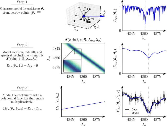
Figure 1. The steps required to produce the model spectrum Mλ,o(θ∗,θs,c). This figure is intended to clarify the mathematical
nomenclature and visualise the data-generating procedure. Transformations occur from left-to-right, starting from the top row. The spectrum in the top right is a high-resolution (R ∼20,000) portion surrounding Hα, which is marked in all panels in the rightmost column. The inset axes in the center panel shows a 5×5 ˚A zoom-in of the convolution kernel. Redder wavelengths have a larger kernel width due toR. Positive redshifts move the position of the diagonal convolution to the right. The final model spectrum is shown compared to a low-resolution (R ∼2,000) spectrum of a solar-like star with S/N∼30 per pixel. The additional nuisance parameters f,pb,vbonly contribute during the calculation of the likelihoodL, and do not affect the data generated by the model.
p(θ∗,dim) =U
minh{θ∗}griddim
i
,maxh{θ∗}griddim
i (10) p(z,{c}) = 1 (11) p(lnf) =U(−10,1) (12) p(pb) =U(0,1) (13) p(R, vb) =
1,for values greater than zero
0,otherwise (14)
There are some subtleties to enforcing p(θ∗). A con-sequence of allowing irregular model grids in the N -dimensional linear interpolation model is that occasion-ally a spectrum cannot be interpolated for someθ∗, even
if it is bound within minh{θ∗}griddimi,maxh{θ∗}griddimi because it will be outside the convex hull. In these cases p(θ∗) = 0 and thus lnP = −∞. On the other hand
if a Cannon spectral model is used, data can be pro-duced beyond the strict parameter limits that make up the training set. Although this is not a severe restriction
onThe Cannon, by defaultsickis cautious and enforces p(θ∗) = 0 for points outside the limits of the training set.
This option can be disabled by the user.
It is clear that the priors on{c}intuitively should not be uniform. Higher order terms of a polynomial sequence should have much smaller priors, as their absolute mag-nitudes are expected to be much smaller than lower or-der terms. In practice the initialization of continuum parameters is normally sufficient such that the default uniform priors on {c} pose no problem, but for the ex-pert user there is clearly room for a formal, well-founded prior to be enforced on {c}, which can be enabled in thesick model description. Finally, negative generated model fluxesMλ,oare considered unphysical, and set to
non-finite values.
2.7. The Likelihood Function
The likelihood function has an additional term if out-lier pixels are treated with a mixture model. The param-eter Θ ≡ [θ∗, vsini,R,z,{c},f] describes all parame-ters in the model. If a Cannon model is used, the
im-plication is that the parameters{θλ,m,sλ,m}have been
solved for at each pixel, and are thus already folded in to Iλ,m(θ∗) and s2λ,o. Similarly, due to the convolution
and binning matrix S, the model flux at a given pixel λo,i is reliant on knowing the neighbouring model and
observed wavelengths λm and λo, but for brevity I do
not explicitly specify these terms in Equation 15 below. I can now describe the frequency (or probability dis-tribution) for the flux at each pixel (of {λo, Fλ,o, σλ,o})
p(Fλ,o|λo,σλ,o,Θ) for the observed dataFλ,o:
p(Fλ,o|λo,σλ,o,Θ) =
1
q
2πs2
λ,o
exp −[Fλ,o−Mλ,o]
2 2s2 λ,o ! (15) wheres2
λ,owas defined in Equation 9. If the outlier pixels
are also being modelled then the probability distribution forFλ,o becomes a mixture of two models:
p(Fλ,o|λo,σλ,o,Θ, pb, vb) =· · ·
(1−pb)×p(Fλ,o|λo,σλ,o,Θ) +· · ·
pb×pbackground(Fλ,o|λo,σλ,o,Θ, vb)
(16) Wherepbackground is defined as:
pbackground(Fλ,o|λo,σλ,o,Θ, vb) =· · ·
1
q
2π(s2
λ,o+vb)
exp −[Fλ,o−Cλ,o]
2 2[s2 λ,o+vb] ! (17) 3. METHODOLOGY
sick aims to be flexible to achieve different scientific objectives, depending on the data volume and the com-puting resources available. Generally, when I have ac-quired some data, I seek either a coarse guess of the model parametersΘ, a numerically-optimised point es-timate of Θ (no uncertainties), or full sampling of the posterior probability distribution. sick has three pri-mary analysis functions to suit these scenarios. Below I list the abridged sick command line usage for each situation, as well as a brief description:
1.sick estimate <model> <data>
An initial estimate of the model parameters
Θestimateis obtained by cross-correlating a
pseudo-normalised copy of the data against the entire model grid (or some subset thereof; Section 3.1). The nearest neighbourθnearest
∗ is returned, and{c}
and zare estimated from θnearest
∗ .
2.sick optimise <model> <data>
Numerical optimisation of −lnP begins from
Θestimate, unless an initial guess is provided. If
no minimisation algorithm is selected, a scaled and bounded version of the Broyden, Fletcher, Gold-farb, and Shanno (BFGS; Section 3.2) algorithm is used.
3.sick infer <model> <data>
Markov Chain Monte Carlo (MCMC) sampling
begins from the numerically optimised point
Θestimate. Sampling occurs for at least 2,000
steps with 200 walkers (4×10⁵ probability
evalua-tions), with convergence automatically determined from the autocorrelation functions, unless conflict-ing samplconflict-ing requirements have been provided by the (presumably expert) user.
3.1. Initial Estimate
I require a good initial estimate of the model param-eters Θestimate. Initially sick fits each observed
chan-nel with a polynomial (with degree set by the user in the model configuration file), discards pixels that devi-ate by more than 4σ, and repeats the fit. A copy of the data is divided by the fitted continuum, yielding a ‘pseudo-normalised’ spectrum (e.g., the spectrum is ‘nor-malised’ without any consideration of strong molecular bands or continuous opacities depressing the entire spec-trum)5. This ‘pseudo-normalised’ spectrum is then cross-correlated against the entire model grid, or Ngrid estimate
equispaced points across {θ∗}grid.
The relative peak of the cross-correlation function (CCF) Fmo provides a reliable metric of similarity
be-tween two spectra, thereby providing a cheap estimate of the model parameters θ∗. Given the nearest-neighbour guess of θ∗ and the redshift z, the optimal continuum coefficients c can then be calculated algebraically after pseudo-sampling (i.e., interpolating)Iλ,m(1+z)on toλo:
Fλ,o≈Iλ,m(1+z)(θ∗)·Cλo(c,λo) (18)
When multiple channels are present (and the redshift is being modelled separately in each channel), an estimate of the closest model parameters θ∗ is provided by each
channel. In this scenario sick calculates the optimal continuum coefficientscin each channel, for each unique value of the set {θ∗} returned from the peaks of the CCFs.
The χ2 difference (calculated using all channels)
be-tween the approximate model (Equation 18) and the data is calculated for each entry in θ∗. The point with the lowest total χ2 value is taken as the initial estimate of θ∗ (and its corresponding redshift(s) z and continuum
coefficients {c}). The spectral resolution(s) R are esti-mated from the wavelength spacing ∆λλ in each channel. The fraction of underestimated variance is assumed to be high (lnf = 0.5), and the outlier fraction is initially estimated to be small (1%), with the outlier variance as-sumed to be comparable to the observed pixel variance vb=hσλ,oi2.
3.2. Optimisation
The model parameters Θ are then numerically opti-mised, using Θestimate as the starting point. I
numeri-cally optimise the parametersΘby minimising the nega-tive log-probability−ln (P). A number of suitable min-imisation algorithms are available in sick through the SciPy (Jones et al. 2001) optimization module:
• BFGS (Byrd et al. 1995; Zhu et al. 1997; Morales & Nocedal 2011; Nocedal & Wright 2006) [default] 5 This procedure constitutes the antithesis of an earlier
foot-note, but is only being performed to facilitate a cheap comparison between the data and all possible models.
• Modified Powell’s method (Powell 1964; Press et al. 2002)
• Non-linear conjugate gradient method (Nocedal & Wright 2006)
• Truncated Newton conjugate-gradient method (Nash 1984; Nocedal & Wright 2006)
• Nelder-Mead (Nelder & Mead 1965)
If bounded information is available (e.g., boundaries of
{θgrid∗ }or limits from uniform priors),sickwill use con-strained implementations of the algorithms above, where they exist. For algorithms that utilise a single parame-ter scaling factor for gauging convergence (e.g., factr in BFGS), sickautomatically scalesΘto place the pa-rameters in the same order of magnitude. Tunable con-vergence parameters for each optimisation algorithm are also configurable through the model configuration file. However, the default options insick should be suitable for most purposes.
Model parameters can also be optionally fixed during the optimisation process. For example, if only a point es-timate of Θis required (e.g., no MCMC sampling) and the procedure in Section 3.1 provides a reliable measure ofz, one might choose to keep z fixed for the optimisa-tion process and solve for the remainingΘ.
3.3. Monte-Carlo Markov Chain Sampling The aforementioned steps efficiently provide an accu-rate point estimate of the optimal parametersΘoptimised.
However they do not provide a measure of uncertainty on
Θ, which is usually more important than a single value6. sick employs the affine-invariant ensemble Metropolis-Hastings sampler proposed by Goodman & Weare (2010) and implemented by Foreman-Mackey et al. (2013). The initial distribution ofΘ(hereafter called the initial state α) are drawn from a small multi-dimensional ball around the optimised parametersΘoptimised.
Before the posterior distributions ofΘcan be properly sampled, the MCMC chains must be thermalised (i.e., ‘burnt in’) from the initial proposalαto the equilibrium distributionπ. It can be shown (e.g., Chung 2006) that a Markov chain will converge to π as t→ ∞. However the initial transit period fromαtoπmust be discarded; our posteriorp(Θ) should not depend on the initial dis-tributionα. Ensuring a Markov chain converges to equi-librium in finite time is a fundamental topic in statistics. In an attempt to make sick easy to use, some de-fault behaviour has been introduced to routinely eval-uate whether convergence has probably been achieved. Consider the transit from theαtoπdistributions. Each successive state (Θo, Θ1, . . .) of the Markov chains are
correlated. In other words, each state depends slightly 6A useful analogy to emphasise the importance of uncertainties
is a hypothetical scenario where you are told a measure of some unfamiliar physical object, without being told theunitof measure. Without knowing anything about the object (e.g., rough size, its purpose, etc), the measure could be miles, volume in mm3,
temper-ature – you don’t know! Similarly if I measured some astrophysical quantity (one which could be expressed in a variety of units) to be X – it’s equally uninformative to omit the uncertainties as it is to omit the units! There is no information about thescaleorvariance ofX. Uncertainties are important.
on the previous state. This is the exact opposite of what I actually want to achieve, as I seek π to be effectively independent of the initial distributionα. Thus the auto-correlation between successive states is informative of – amongst other things – whether the Markov chains are near αor π. If one considers an observablef (e.g., any parameter inΘ), I can estimate its mean,
hfi=
Z
f(φ)p(φ)dφ (19)
where p(φ) is the probability density function. The un-normalised autocorrelation function Cf f between two
successive statest−1 andt is then given by:
Cf f(t)≡ hft−1fti −µ2f (20)
=X
x,y
f(x)[πxpxy(|t|)−πxπy]f(y)
(21) What is of most interest is thenormalised autocorrela-tion funcautocorrela-tionρf f(t) at a given time stept, as normalised
to the initial (t = 0) state α. That is to say, the nor-malised autocorrelation functionρf f(t) provides a
mea-sure of how correlated a value f (at time t) is to the initial distributionα(whent= 0):
ρf f(t)≡ Cf f(t)
Cf f(0) (22)
The normalised autocorrelation function will decay ex-ponentially for large t as the states move closer to the equilibrium distributionπ. In other words, at some large t (which is unknowna priori) the stateΘtwill be
inde-pendent, or negligibly dependent on the initial state α. Therefore it is important to knowhow quickly the expo-nential decay ofρf f is, such that I can identify where the
chains have properly thermalised and settled in to ∼π. Theexponential autocorrelation timeτexp,f provides the
measure of decay and is defined as, τexp,f = lim
t→∞sup t
−ln|ρf f(t)|
(23) whereτexpprovides the relaxation time of the system, as
given by which parameterf is moving slowest fromαto π:
τexp= sup f
τexp,f (24)
Therefore, ift is large enough, the burn-in period can be estimated as a∼few multiples of the relaxation time of the system τexp. However there is some ambiguity
about when τexp can be calculated, because for short
chains τexp is forced to be shorter than the chain length
by construction. For this reason we must sample a ‘suffi-cient’ number of times before estimating the exponential autocorrelation time. Adopting conservative behaviour by default,sick will initialize 200 walkers and run until τexp <1/64 the chain length. In practice this may be
overkill, but this behaviour can be changed by the user. I estimateτexp by first calculating the normalised
8500 8600 8700 8800 Wavelength,λo[ ˚A] 0 800 1600 2400 3200 Coun ts [-]
Figure 2. A faux observed spectrum (black) ofR ∼20000 and S/N ratio of∼20 per pixel, which was used in the toy model test. The
recovered maximum a posteriori model spectrum is shown in red.
mean position of all walkers at any time t. For any timetI take the maximum absolute ρf f for any
param-eter f: ρmax = supf|ρf f|. Thus, ρmax gives the upper
limit of autocorrelation in any parameter f at a given timet. Finally, I fit an exponential function of the form exp− t
τexp
to the profile (t, ρmax) by least-squares
min-imisation in order to estimateτexp.
Given the estimate of τexp I discard the first
3×τexp MCMC steps as the thermalisation phase.
Using the remaining samples, I next calculate the integrated autocorrelation time τint (using the
emcee.autocorr.integrated time function), which is distinct from the exponential autocorrelation time discussed above. The integrated autocorrelation time is defined as: τint,f= 1 2+ ∞ X t=1 ρf f(t) (25)
Because the integrated autocorrelation time τint,f is
calculated only on samples after 3×τexp(i.e., after
ther-malisation has occurred), it provides a measure of the statistical error in the Monte Carlo samples of parameter
hfi, and a means of determining the number of effective independent samples off,
Nef f,f ≈
Nsteps
2τint,f
(26) where Nsteps is the number of production
(post-thermalisation) MCMC steps. The reader is referred to the excellent notes by A. D. Sokal7 for more details (and
clear derivations) of sample estimators and autocorrela-tion times.
After the thermalisation regime has been identified, the default constraint for convergence in sick is to have more than 100 effective independent samples in every parameter f. If this heuristic is not met after the first 2,000 steps, sick will calculate τexp, τint and
Nef f every 1,000 MCMC steps thereafter. Expert users
can modify this behaviour by disabling convergence checking completely (with the auto convergence set-ting) in lieu of specifying the number of iterations to burn and sample, or by altering the following con-vergence criteria settings: n tau exp as burn in, minimum effective independent samples,
7http://www.stat.unc.edu/faculty/cji/Sokal.pdf
check convergence frequency, andminimum samples, which will specify the minimum number of MCMC steps before evaluating convergence.
Once sampling is complete, sick generates figures showing the normalised auto-correlation ρf f in each
pa-rameter, the mean acceptance fraction at each step, all of the sampled Θparameters in each chain, corner plots showing marginalised posteriors forΘandθ∗, as well as projection (spectrum) plots that illustrate the quality of fit to the data. Furthermore, the chains and final state of every MCMC is saved bysick, allowing users to resume their analysis from the most recent state, calculate ad-ditional sample estimators, or to produce supplementary post-processing figures.
4. TOY MODEL
A straightforward test of the probabilistic framework described above is to produce a noisy faux observa-tion, and infer the model parameters Θ, given the faux data. The AMBRE public spectral library (de Laverny et al. 2012) has been employed as the grid of model intensities. I used ∼4000 points {θ∗}grid
in the range 4000 < Teff < 8000, 0 < logg < 5, −3 < [Fe/H] < 0.5 and −0.2 < [α/Fe] < 0.8 to train a Cannon quadratic-in-labels model with linear cross-terms. Stellar parameters {Teff,logg,[Fe/H],[α/Fe]} of
a solar-like star θ∗ = [5841,4.41,−0.03,+0.01] were chosen, and model intensities Iλ,m were generated
be-tween λm = [8450,8900] ˚A. The wavelength range is
quite common to many surveys and instruments: RAVE, FLAMES/GIRAFFE (HR21), Gaia RVS, AAOmega (1700I/D). For this test, the spectral resolution is most comparable to FLAMES/GIRAFFE. For the purposes of producing a faux observation, I disregard the uncertain-ties in producing the model intensiuncertain-ties σλ,m. In other
words, σλ,m does not contribute to thequoted noise in
σλ,o. However when generating model intensities for
probability evaluations at run-time,σλ,menters into the
likelihood function as per Equation 9.
A number of transformations were then applied to the intensities. The spectra were convolved to a resolving power ofR ∼20,000 and redshifted by a random veloc-ity drawn from N(0,300) km s−1 before the data were
binned onto a uniform spacing of 0.1 ˚A. A second-order polynomial was used to represent the continuum, and noise was added to replicate a S/N ratio of ∼ 20 per pixel.
The model included the parametersTeff, logg, [Fe/H],
0 2000 4000 6000 8000 10000 MCMC step,t −0.5 0.0 0.5 1.0 ρff ( t ) ≡ Cf f ( t ) /C f f (0)
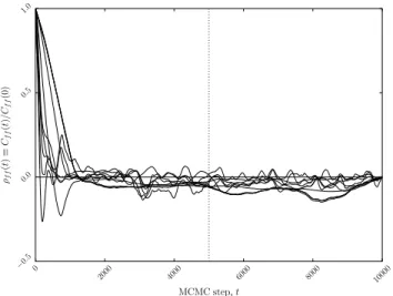
Figure 3. The normalised autocorrelation functionρf ffor the toy
model. Auto-correlations from all model parameters are shown, as calculated by the mean position of the walkers at each time stept. The exponential autocorrelation time isτexp∼500, demonstrating
that the Markov Chains are in equilibrium (converged) well before the burn-in point,t= 5000 (marked).
5000 steps to thermalise the sampler. In practice, this is more samples than what was necessary for this test, as evidenced by the normalised autocorrelation function ρf f(t) (Figure 3). The chains were reset and another
5000 MCMC steps were performed to sample the poste-rior distribution. The posteposte-rior probability distributions of θ∗ are shown in Figure 4, where blue marks the
pa-rameters used to generate the data. Table 1 lists the maximum a posteroiri values ofΘ(which is projected to the data in Figure 2) and the 16th and 84th percentiles of theΘdistributions. It is clear from Figure 4 and Ta-ble 1 that the model recovers the data-generating values
Θvery well.
5. UTILITY: ATOMIC DIFFUSION IN M67
Although sick can be used to estimate a (nearest-neighbour or numerically optimised) point estimate, I have spent considerable effort describing the dominant conceivable phenomena that may affect the data, and outlined how to incorporate those nuisance effects into a scalar-justified model. Given the additional (often considerable) computational cost implied by MCMC to marginalise over these nuisance parameters, it is reason-able to ask ‘Why bother?’. Does the introduction and marginalisation of nuisance parameters actually improve our inferences on astrophysical parametersθ∗? In other words, if a full sampling of the posterior and marginal-isation of nuisance parameters does not provide addi-tional scientific information, is it pragmatic to perform MCMC? The computational cost may not be warranted. Here I present a suitable application that demonstrates that there is additional information in existing public spectra which has not been fully exploited. M67 is a nearby (∼800-900 parsec; Sandquist 2004; Majaess et al. 2011; Sarajedini et al. 2009; Yakut et al. 2009) open cluster with a near-solar metallicity: [Fe/H] =−0.04 to +0.03 (Hobbs & Thorburn 1991; Tautvaiˇsiene et al. 2000; Yong et al. 2005; Randich et al. 2007; Pace et al. 2008; Pasquini et al. 2008; ¨Onehag et al. 2011). The age of the cluster is comparable to the Sun (3.5−4.8 Gyr), and rep-resents an excellent test-bed for stellar evolution and
dif-fusive convection at solar metallicity (e.g., VandenBerg et al. 2008).
Candidate stars in M67 were observed on the Aus-tralian Astronomical Telescope with the AAOmega in-strument in May 2011. The 1700D grating was used in the red arm, which gives comparable wavelength cover-age to the toy model in Section 4, but at a lower res-olution of R ∼ 10000. I convolved the AMBRE spec-tral library (de Laverny et al. 2012) to this specspec-tral res-olution while keeping the high-resres-olution sampling. A Cannon model with label vector [1, Teff3, Teff2 , logg2,
[Fe/H]2, [α/Fe]2, Teff · logg, Teff ·[F e/H], Teff ·[α/Fe],
logg·[α/Fe], [Fe/H]·[α/Fe], Teff, logg, [Fe/H], [α/Fe]]
was trained across the region 4000 <= Teff <= 7000,
1.0 <= logg <= 5.0, −2.5 <= [Fe/H] <= 0.5, and
−0.4 <= [α/Fe] <= 0.4 (4202 points). Once the model was trained, I used the ‘sick infer’ command line (with prescribed ‘burn’ and ‘sample’ values, see be-low) to infer astrophysical parameters given the 1700D spectra. As described in Section 3, the −lnP was nu-merically optimised from a nearest-neighbour point esti-mate of the parameters Θ, before performing MCMC sampling with 200 walkers for 2000 steps in thermal-isation and production. The model parameters were
Θ= [Teff,logg,[Fe/H],[α/Fe], z,R,lnf, c0, c1, c2, pb, vb].
Cluster members were unambiguously identified from their inferred redshifts z. Suspected spectroscopic bi-naries (due to significant line broadening or resolved double-peaks in their spectrum) were discarded. The distilled sample includes 24 members, which are shown in Figure 5, with a 4.5 Gyr solar-metallicity PARSEC (Bressan et al. 2012) isochrone to guide the eye. The sample consists of predominantly turn-off and sub-giant stars. The discrepancy with the isochrone at the giant branch is a noticeable, well-studied effect (e.g., Vanden-berg 1983). Indeed, the position of the red giant branch is a sensitive function of the (invoked) α parameter in mixing length theory. For this reason M67 has been a useful boundary condition for testing blanketed model atmospheres (e.g., VandenBerg et al. 2008). Without this condition, the position of the red giant branch in 4.5 Gyr solar isochrones tends redwards (e.g., cooler temper-atures), to the same degree that I find in Figure 5. The uncertainties are sufficiently large that I cannot precisely distinguish between stars that have passed the turn-off point, but the overall agreement with the sequence is satisfactory.
If I assume that the underlying metallicity distribu-tion of M67 is a Gaussian, and account for the uncer-tainties in [Fe/H] for each star, from all cluster members I find the metallicity of M67 to be [Fe/H] =−0.06. This measurement is in reasonable agreement with existing studies that place the metallicity of M67 between −0.04 and +0.03. However, Figure 5 shows the sample is two-thirds dominated by turn-off stars. In Figure 6 I show the inferred maximum a posteriori metallicity for all M67 stars, binned to 0.05 dex increments (i.e., roughly equiv-alent to the uncertainties in individual measurements). The turn-off and sub-giant stars are colored in the same way as Figure 5, and the hatching represents an overlap between the two distributions. As a whole, the turn-off stars are more metal-poor than the sub-giant stars. If the uncertainties in [Fe/H] for each star are considered,
4.2 4.3 4.4 4.5 4.6 log g −0. 10 −0. 05 0.00 0.05 [F e / H] 5680 5760 5840 5920 Teff[K] −0. 03 0.00 0.03 0.06 0.09 [ α/ F e] 4.2 4.3 4.4 4.5 4.6 logg −0. 10 −0. 05 0.00 0.05 [Fe/H] −0. 03 0.00 0.03 0.06 0.09 [α/Fe]
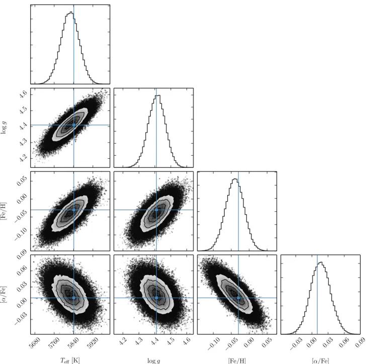
Figure 4. Posterior probability distributions for all astrophysical parametersθ∗for a faux observation with spectral resolutionR ∼20,000
and S/N ratio∼20 per pixel. The posterior probability distributions ofθ∗are marginalised overz,R,cand lnf. The parameter values used to generate the data are marked in blue. This figure demonstrates the forward model described, and highlights how precise inferences of stellar parameters can be made with high-resolution spectra, even in the presence of substantial noise.
and assume the underlying metallicity distribution in the sub-giant and turn-off sample are normally distributed, I find the metallicity of turn-off stars to be [Fe/H]=−0.07, and [Fe/H]=−0.02 for the sub-giant stars.
The difference in metallicities between sub-giant and turn-off stars in M67 is not a new result. ¨Onehag et al. (2014) performed a differential study of sub-giant and turn-off stars in M67 with respect to the solar twin M67-1194. Their data were obtained from the UVES instru-ment on the VLT, providing R ∼ 47,000 and S/N ∼ 150 per (binned) pixel. This data quality permitted the
determination of individual chemical abundances in a strictly differential sense. It is important to remember that the metallicity difference I find is probably a convo-lution of multiple elements within this wavelength range (Fe, Ti, and Ni). With this caveat in mind – and al-though ¨Onehag et al. (2014) cover a slightly different temperature range – the effect I find is the same: heavy-element abundances (including Fe) in M67 are found to be reduced in the hotter stars and dwarfs by typi-cally ≤0.05 dex, as compared to the abundances of the sub-giants. Thus, with an objective characterisation of
Table 1
Model parameters and values employed for, and inferred from, the toy model.
Parameter Description Data-Generating Value MAP Value
Teff Effective photospheric temperature [K] 5841 5825+38−38
logg Surface gravity 4.41 4.41+0−0..0505
[Fe/H] Metallicity −0.03 −0.04+0−0..0303
[α/Fe] α-element enhancement +0.01 +0.02+0.02
−0.02 z·c Redshift/Doppler shift [km s−1] 43.1 43.2+0.1
−0.4
R Spectral resolution 20000 21648+232−1446
c0 Continuum polynomial coefficient −8000 −9050+2335−2358 c1 Continuum polynomial coefficient 1.14 1.39+0−0..5454 c2 Continuum polynomial coefficient (×10−5) −5 −1.42+3−3..1114
lnf Logarithm of fractionally underestimated variance · · · −8.93+0−0..8573
4500 5000 5500 6000 6500 Teff[K] 1.5 2.0 2.5 3.0 3.5 4.0 4.5 5.0 log g
Sub-giant stars Turn-off stars
Figure 5. Inferred effective temperatures and surface gravities of
confirmed cluster members of M67. A single-mass 4.5 Gyr PAR-SEC (Bressan et al. 2012) isochrone of solar metallicity is shown to guide the eye. The discrepancy in the position of the red gi-ant branch is a known astrophysical phenomena (see text). When accounted for, there is good overall agreement with the sequence. Samples are labelled as turn-off or sub-giant stars.
−0.15 −0.10 −0.05 0.00 0.05 0.10 0.15 [Fe/H] 0 2 4 6 8 Coun t
Sub-giant stars Turn-off stars
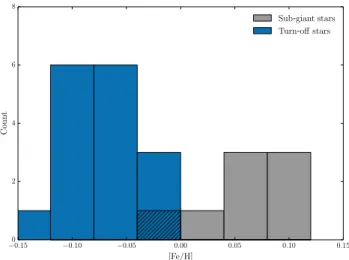
Figure 6. A histogram showing the maximum a posteriori
metal-licity for confirmed M67 stars, colored by their evolutionary stage as per Figure 5. As a whole, the sub-giant stars exhibit slightly (+0.05 dex, when individual uncertainties in [Fe/H] are considered) higher metallicities than the turn-off stars, a result previously iden-tified from high-resolution spectra by ( ¨Onehag et al. 2014) and attributed to atomic diffusion.
(most) dominant phenomena that will affect the obser-vations, subtle astrophysical phenomena can be inferred from lower-resolution spectra than what is typically con-sidered. This example application shows, to a large ex-tent, that existing stellar spectroscopic data are suffi-ciently high-quality that the standard of our results will be dominated by our analysis methods. For this reason, a move towards generative models in stellar spectroscopy is essential.
6. DISCUSSION
Here I discuss some future applications that forsick, an important potential caveat, and outline planned near-term improvements for the code.
6.1. Further Applications
As previously discussed,sick is agnostic about wave-length coverage, resolving power, or binning of the ob-served data. This generality allows for an extremely high-resolution grid to be used for many applications of lower resolutions, as long as the wavelengths are covered. For example, the same high-resolution library (observed or synthetic) can be used for surveys of high-resolution (e.g., APOGEE), low-resolution (e.g., SEGUE, Gaia RVS or Gaia BP/RP8 – whereR ∼120), placing stars
from all surveys on the same, self-consistent scale. The flexibility in methodology (e.g., estimate, optimise, infer) also allows for quick analyses over extremely large data sets (e.g., LAMOST) to identify superlative objects with high scientific impact (e.g., ultra metal-poor or hyper-velocity stars). Similarly, large collections of point estimates can be sufficient to identify and quantify substructure in the Milky Way halo. Alternatively, sampling posterior probability distributions for a reasonable sample of cluster stars may reveal subtle abundance variations, helping to untangle the ‘multiple population’ scenario (e.g., see Carretta et al. 2009, and references therein) or understand the effects of atomic diffusion in clusters of different ages and metallicities.
6.2. Caveats
8 Indeed, sick performed excellently in a blind test
dur-ing the 3rd Gaia Challenge Workshop, slightly outperform-ing the current BP/RP analysis method for metal-poor stars:
http://astrowiki.ph.surrey.ac.uk/dokuwiki/doku.php?id=tes ts:astropars:challenge3
Although there are substantial scientific applications for the tool presented here, there is an obvious caveat that requires attention. The examples here have focused on producing model intensities Iλ,m from at most four
dimensions. As the number of dimensions increase – for example, to include individual chemical abundances – thecurse of dimensionalitywill quickly become relevant. The computational complexity in producingIλ,m scales
quickly, such that a linear interpolation model will be-come absolutely unsuitable in higher dimensions. On the other hand, there are some tricks that can be introduced for a Cannon-like approach in high-dimensionality for chemical abundances (e.g., see Ness et al. 2016; Casey et al. 2016). Alternatively, compounding two suitable models may be a reasonable scenario: one for the deter-mination of stellar parameters, and another that pro-duces spectra of individual elemental abundances (by some means,Cannon-like or synthesised) for some small wavelength region and stellar parametersθ∗. The
abun-dance of an individual element can be marginalised over all possible θ∗. The implied assumption here is that the individual chemical abundances do not have a sub-stantial effect on the overall stellar parameters. It is tempting to assert that this is an unwarranted general-isation. However this is an implied assumption used in the production of model photosphere, since the photo-spheres themselves are calculated with a given chemical composition of individual elements. Although there are potential ways to deal with higher dimensionality (in stel-lar applications), extreme care must be made in scaling the intensity-generating methods described here.
There are a number of caveats that users must be cog-nisant of even for models with low-dimensionality. These apply to the data and the model employed. For exam-ple, this framework is most suitable for one-dimensional extracted spectra; it is beyond the scope of this work to forward model two-dimensional images. Likewise, sick may be sub-optimal for echelle spectra with many or-ders due to the high number of{c} coefficients that are physically related.
Even within a single order, there are strong assump-tions made about the line spread function. It is assumed that the resolution scales (at most) linearly with wave-length, which can be shown to be knowingly incorrect for most spectrographs. The effect of this assumption will usually be small (a small second order resolution term is probably warranted), but it should be known.
In the work presented here, flux noise is assumed to be Gaussian. Similarly the noise can only assumed to be under-estimated (not over-estimated), and no frame-work has been presented to account for correlated noise between neighbouring pixels (e.g., Czekala et al. 2014). It is also important to note that the treatment of outliers in this work may be overkill: rejecting highly discrepant pixels may be sufficient. In short, the user should be ex-tremely familiar with the model description they set out for the data, and the limitations thereof. Improvements to the code that help resolve these existing caveats are welcomed in the form of pull requests through GitHub9.
7. CONCLUSION
9github.com/andycasey/sick
I have presented a flexible probabilistic code to for-ward model spectroscopic data. The generative model approach described here has a number of advantages over previously published techniques. Preparatory and subjective decisions (e.g., redshift and placement of con-tinuum) are objectively treated within a scalar-justified mathematical model, allowing for a credible assessment of uncertainties in astrophysical parameters. Almost all previously published techniques have treated these pro-cesses separately, thereby increasing biases in their re-sults and generally mis-characterising the uncertainties in astrophysical parameters.
The simultaneous incorporation of continuum, red-shift, convolution and resampling leads to remarkable improvements in both accuracy and precision. While the examples presented here have focused on stellar spectra, the code is ambivalent aboutwhat the astrophysical pa-rameters describe: the framework can be easily used for any kind of quantifiable astrophysical process. The code is MIT-licensed (freely distributable, open source) and has an extensive automatic testing suite. Complete doc-umentation is available online, which includes a number of additional examples and tutorials on analysing data from well-known stellar surveys (e.g., SEGUE, LAM-OST, APOGEE).
Great effort has been made to ensure the code is easy to use, allowing users to obtain precise inferences with little effort. I strongly encourage the use of this software for existing and future spectral data. With the sheer volume of high-quality of spectra available, astronomers must begin to adopt objective, generative models for their data. Subtle astrophysical processes can only be discovered and understood with the proper characterisa-tion of uncertainties afforded by generative models.
I am pleased to thank Matt Auger, Sergey Ko-posov, Melissa Ness, Jarryd Page, Jason Sanders, and Kevin Schlaufman. I am particularly indebted to Brian Schmidt for introducing me to Bayesian statistics and generative models (far too late, I might add), and to the referees for their constructive and direct criticism, which improved the methodology of the code and overall clarity of this paper. This research has made extensive use of NASA’s Astrophysics Data System Bibliographic Services, the Coveralls continuous integration service, GitHub, and the triangle.py code (Foreman-Mackey
et al. 2014). The author recognises support through the European Research Council grant 320360: The Gaia-ESO Milky Way Survey. The source code for this re-search is distributed using git, and is hosted online at
GitHub. Suggestions for improvements or unexpected behaviour can be reported through GitHub issues, and code contributions are welcomed in the form of pull re-quests.
REFERENCES
Allende Prieto, C., Sivarani, T., Beers, T. C., et al. 2008, AJ, 136, 2070
Barber, C. B., Dobkin, D. P., & Huhdanpaa, H. 1996, ACM TRANSACTIONS ON MATHEMATICAL SOFTWARE, 22, 469
Blondin, S., & Tonry, J. L. 2007, ApJ, 666, 1024
Byrd, R. H., Lu, P., Nocedal, J., & Zhu, C. 1995, SIAM J. Sci. Comput., 16, 1190
Carretta, E., Bragaglia, A., Gratton, R. G., et al. 2009, A&A, 505, 117
Casey, A. R., Hogg, D. W., Ness, M. K., & Rix, H.-W. 2016, in preparation
Chung, K. L. 2006, Markov Chains With Stationary Transition Probabilities
Cui, X.-Q., Zhao, Y.-H., Chu, Y.-Q., et al. 2012, Research in Astronomy and Astrophysics, 12, 1197
Czekala, I., Andrews, S. M., Mandel, K. S., Hogg, D. W., & Green, G. M. 2014, ArXiv e-prints, arXiv:1412.5177
de Laverny, P., Recio-Blanco, A., Worley, C. C., & Plez, B. 2012, A&A, 544, A126
De Silva, G. M., Freeman, K. C., Bland-Hawthorn, J., et al. 2015, MNRAS, 449, 2604
Drinkwater, M. J., Jurek, R. J., Blake, C., et al. 2010, MNRAS, 401, 1429
Foreman-Mackey, D., Hogg, D. W., Lang, D., & Goodman, J. 2013, PASP, 125, 306
Foreman-Mackey, D., Price-Whelan, A., Ryan, G., et al. 2014, doi:10.5281/zenodo.11020
Gilmore, G., Randich, S., Asplund, M., et al. 2012, The Messenger, 147, 25
Goodman, J., & Weare, J. 2010, Comm. Appl. Math. Comp. Sci., 5, 65
Gray, D. 2005, The Observation and Analysis of Stellar Photospheres (Cambridge University Press)
Hobbs, L. M., & Thorburn, J. A. 1991, AJ, 102, 1070
Husser, T.-O., Wende-von Berg, S., Dreizler, S., et al. 2013, A&A, 553, A6
Jones, E., Oliphant, T., Peterson, P., et al. 2001, SciPy: Open source scientific tools for Python, [Online; accessed 2014-07-14] Kerzendorf, W. E., Yong, D., Schmidt, B. P., et al. 2013, ApJ,
774, 99
Kordopatis, G., Gilmore, G., Steinmetz, M., et al. 2013, AJ, 146, 134
Le Borgne, D., Rocca-Volmerange, B., Prugniel, P., et al. 2004, A&A, 425, 881
Lee, Y. S., Beers, T. C., Sivarani, T., et al. 2008, AJ, 136, 2022 Majaess, D. J., Turner, D. G., Lane, D. J., & Krajci, T. 2011,
Journal of the American Association of Variable Star Observers (JAAVSO), 39, 219
Majewski, S. R., Wilson, J. C., Hearty, F., Schiavon, R. R., & Skrutskie, M. F. 2010, in IAU Symposium, Vol. 265, IAU Symposium, ed. K. Cunha, M. Spite, & B. Barbuy, 480–481 Morales, J. L., & Nocedal, J. 2011, ACM Trans. Math. Softw., 38,
7:1
Nash, S. G. 1984, SIAM Journal on Numerical Analysis, 21, 770 Nelder, J. A., & Mead, R. 1965, The Computer Journal, 7, 308 Ness, M., Hogg, D. W., Casey, A. R., & Rix, H.-W. 2016, in
preparation
Ness, M., Hogg, D. W., Rix, H.-W., Ho, A., & Zasowski, G. 2015, ArXiv e-prints, arXiv:1501.07604
Nocedal, J., & Wright, S. J. 2006, Numerical Optimization, 2nd edn. (New York: Springer)
¨
Onehag, A., Gustafsson, B., & Korn, A. 2014, A&A, 562, A102 ¨
Onehag, A., Korn, A., Gustafsson, B., Stempels, E., & Vandenberg, D. A. 2011, A&A, 528, A85
Pace, G., Pasquini, L., & Fran¸cois, P. 2008, A&A, 489, 403 Palacios, A., Gebran, M., Josselin, E., et al. 2010, A&A, 516, A13 Pasquini, L., Biazzo, K., Bonifacio, P., Randich, S., & Bedin,
L. R. 2008, A&A, 489, 677
Powell, M. J. D. 1964, The Computer Journal, 7, 155 Press, W. H., Teukolsky, S. A., Vetterling, W. T., & Flannery,
B. P. 2002, Numerical Recipes in C++: the art of scientific computing, Second Edition
Randich, S., Primas, F., Pasquini, L., Sestito, P., & Pallavicini, R. 2007, A&A, 469, 163
Recio-Blanco, A., Bijaoui, A., & de Laverny, P. 2006, MNRAS, 370, 141
Sandquist, E. L. 2004, MNRAS, 347, 101
Sarajedini, A., Dotter, A., & Kirkpatrick, A. 2009, ApJ, 698, 1872 Schlegel, D. J., Blanton, M., Eisenstein, D., et al. 2007, in
Bulletin of the American Astronomical Society, Vol. 39, American Astronomical Society Meeting Abstracts, 132.29 Smiljanic, R., Korn, A. J., Bergemann, M., et al. 2014, A&A, 570,
A122
Sousa, S. G., Alapini, A., Israelian, G., & Santos, N. C. 2010, A&A, 512, A13
Steinmetz, M., Zwitter, T., Siebert, A., et al. 2006, AJ, 132, 1645 Stetson, P. B., & Pancino, E. 2008, PASP, 120, 1332
Tautvaiˇsiene, G., Edvardsson, B., Tuominen, I., & Ilyin, I. 2000, A&A, 360, 499
Torres, G., Fischer, D. A., Sozzetti, A., et al. 2012, ApJ, 757, 161 Valenti, J. A., & Piskunov, N. 1996, A&AS, 118, 595
Vandenberg, D. A. 1983, ApJS, 51, 29
VandenBerg, D. A., Gustafsson, B., Edvardsson, B., Eriksson, K., & Ferguson, J. W. 2008, Mem. Soc. Astron. Italiana, 79, 759 Yakut, K., Zima, W., Kalomeni, B., et al. 2009, A&A, 503, 165 Yanny, B., Rockosi, C., Newberg, H. J., et al. 2009, AJ, 137, 4377 Yong, D., Carney, B. W., & Teixera de Almeida, M. L. 2005, AJ,
130, 597
Zhu, C., Byrd, R. H., Lu, P., & Nocedal, J. 1997, ACM Trans. Math. Softw., 23, 550