Proportional hydraulics

Proportional

hydraulics

Textbook

Learning System for Automation and Communications

P T B A

q

q

p

p

p

p

q

v

∆

p

∆

p

 Copyright by Festo Didactic KG, D-73734 Esslingen, 1996

All rights reserved, including translation rights. No part of this publica-tion may be reproduced or transmitted in any form or by any means, electronic, mechnical, photocopying, or otherwise, without the prior

Order No.: 094378

Description: PROP.-H. LEHRB. Designation: D.LB-TP701-GB Edition: 09/95

Layout: 20.12.1995 S. Durz Graphics: D. Schwarzenberger Author: D. Scholz

Chapter 1

Introduction to proportional hydraulics B-3

Table of contents 1.1 Hydraulic feed drive with manual control B-6

1.2 Hydraulic feed drive with electrical control

and switching valves B-7 1.3 Hydraulic feed unit with electrical control

and proportional valves B-8 1.4 Signal flow and components of proportional hydraulics B-10 1.5 Advantages of proportional hydraulics B-12

Chapter 2

Proportional valves: Design and mode of operation B-15 2.1 Design and mode of operation of a proportional solenoid B-17 2.2 Design and mode of operation of

proportional pressure valves B-22 2.3 Design and mode of operation of proportional

flow restrictors and directional control valves B-25 2.4 Design and mode of operation of proportional

flow control valves B-28 2.5 Proportional valve designs: Overview B-30

Chapter 3

Proportional valves: Characteristic curves and parameters B-31 3.1 Characteristic curve representation B-33 3.2 Hysteresis, inversion range and response threshold B-34 3.3 Characteristic curves of pressure valves B-36 3.4 Characteristic curves of flow restrictors and

directional control valves B-36 3.5 Parameters of valve dynamics B-42 3.6 Application limits of proportional valves B-46

Chapter 4

Amplifier and setpoint value specification B-47

4.1 Design and mode of operation of an amplifier B-51 4.2 Setting an amplifier B-56 4.3 Setpoint value specification B-59

B-1

Chapter 5

Switching examples using proportional valves B-63 5.1 Speed control B-65 5.2 Leakage prevention B-71

5.3 Positioning B-71

5.4 Energy saving measures B-73

Chapter 6

Calculation of motion sequence for a

hydraulic cylinder drive B-79

6.1 Flow calculation for proportional

directional control valves B-85 6.2 Velocity calculation for an equal area

cylinder drive disregarding load and

frictional forces B-87 6.3 Velocity calculation for an unequal area

cylinder drive disregarding load and

frictional forces B-91 6.4 Velocity calculation for an equal area

cylinder drive taking into account load and

frictional forces B-98 6.5 Velocity calculation for an unequal

cylinder drive taking into account load and

frictional forces B-104 6.6 Effect of maximum piston force on the

acceleration and delay process B-111 6.7 Effect of natural frequency on the acceleration

and delay process B-115 6.8 Calculation of motion duration B-119

B-2

Chapter 1

Introduction to

proportional hydraulics

B-3

B-4

Hydraulic drives, thanks to their high power intensity, are low in weight and require a minimum of mounting space. They facilitate fast and accurate control of very high energies and forces. The hydraulic cylinder represents a cost-effective and simply constructed linear drive. The combination of these advantages opens up a wide range of applications for hydraulics in mechanical engineering, vehicle con-struction and aviation.

The increase in automation makes it ever more necessary for pres-sure, flow rate and flow direction in hydraulic systems to be control-led by means of an electrical control system. The obvious choice for this are hydraulic proportional valves as an interface between control-ler and hydraulic system. In order to clearly show the advantages of proportional hydraulics, three hydraulic circuits are to be compared using the example of a feed drive for a lathe (Fig. 1.1):

■ a circuit using manually actuated valves (Fig. 1.2), ■ a circuit using electrically actuated valves (Fig. 1.3), ■ a circuit using proportional valves (Fig. 1.4).

Fig. 1.1 Hydraulic feed drive of a lathe

B-5

Fig. 1.2 illustrates a circuit using a hydraulic feed drive with manually actuated valves.

1.1 Hydraulic feed drive with manual control

■ Pressure and flow are to be set during commissioning. To this end,

the pressure relief and flow control are to be fitted with setting screws.

■ The flow rate and flow direction can be changed during operation

by manually actuating the directional control valve.

None of the valves in this system can be controlled electrically. It is not possible to automate the feed drive.

P T B A B A P P P T T M Fig. 1.2 Hydraulic circuit diagram of a manually controlled feed drive

B-6

In the case of electro-hydraulic systems, the directional control valves are controlled electrically. Fig 1.3 shows the circuit diagram of a feed drive using an electrically actuated directional control valve. The oper-ation of the lathe can be automated by means of actuating the direc-tional control valve via an electrical control system.

1.2 Hydraulic feed drive using an electrical control system and switching valves

Pressure and flow cannot be influenced during operation by the elec-trical control system. If a change is required, production on the lathe has to be stopped. Only then can the flow control and pressure relief valve be reset manually.

P T B Y2 Y1 A B A P T P P T M Fig. 1.3

Hydraulic circuit diagram of an electrically controlled feed drive

B-7

automation of pressure and flow control is only possible to a limited extent with electro-hydraulic control systems using switching valves. Examples are

■ the connection of an additional flow control by means of actuating a

directional control valve,

■ the control of flow and pressure valves with cams.

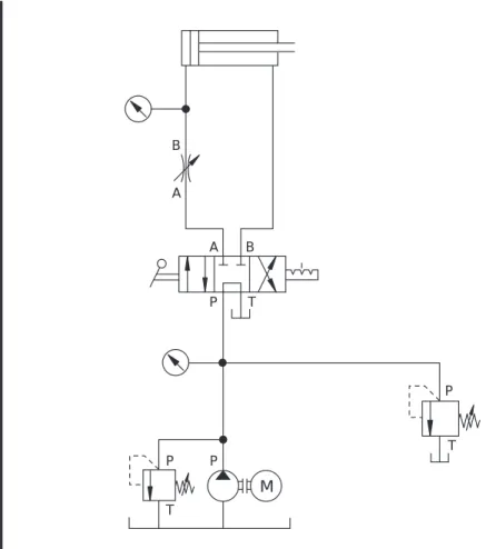
In fig. 1.4 , the hydraulic circuit diagram of a feed drive is shown incorporating proportional valves.

1.3 Hydraulic feed drive using an electrical control system and propor-tional valves

■ The proportional directional control valve is actuated by means of an

electrical control signal. The control signal influences the flow rate and flow direction. The rate of movement of the drive can be infini-tely adjusted by means of changing the flow rate.

■ A second control signal acts on the proportional pressure relief

valve. The pressure can be continually adjusted by means of this control signal.

The proportional directional control valve in fig. 1.4 assumes the function of the flow control and the directional control valve in fig 1.3. The use of proportional technology saves one valve.

The proportional valves are controlled by means of an electrical control system via an electrical signal, whereby it is possible, during operation,

■ to lower the pressure during reduced load phases (e.g. stoppage of

slide) via the proportional pressure relief valve and to save energy,

■ to gently start-up and decelerate the slide via the proportional

direc-tional control valve.

All valve adjustments are effected automatically, i.e. without human intervention.

B-8

P T B Y2 Y3 Y1 A B A P T P P T M Fig. 1.4

Hydraulic circuit diagram of a feed drive using proportional valves

B-9

Fig. 1.5 clearly shows the signal flow in proportional hydraulics.

1.4 Signal flow and components in pro-portional hydraulics

■ An electrical voltage (typically between -10 V and + 10 V) acting

upon an electrical amplifier.

■ The amplifier converts the voltage (input signal) into a current

(out-put signal).

■ The current acts upon the proportional solenoid. ■ The proportional solenoid actuates the valve.

■ The valve controls the energy flow to the hydraulic drive. ■ The drive converts the energy into kinetic energy.

The electrical voltage can be infinitely adjusted and the speed and force (i.e. speed and torque) can be infinitely adjusted on the drive accordingly.

Electrical amplifier

Controller Proportional

solenoid

Proportional technology components

Proportional valve Drive FESTO SPS FESTO FESTO Fig. 1.5: Signal flow in proportional hydraulics

B-10

Fig. 1.6 illustrates a 4/3-way proportional valve with the appropriate electrical amplifier.

Fig. 1.6

4/3-way proportional valve with electrical amplifier (Vickers)

B-11

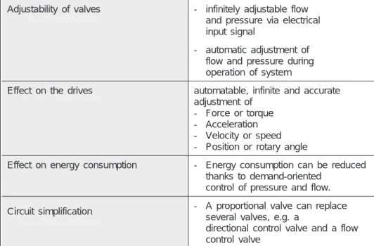
Comparison of switching valves and proportional valves 1.5 Advantages

of proportional hydraulics

The advantages of proportional valves in comparison with switching valves has already been explained in sections 1.2 to 1.4 and are summarised in table 1.1.

Adjustability of valves - infinitely adjustable flow and pressure via electrical input signal

- automatic adjustment of flow and pressure during operation of system

Effect on the drives automatable, infinite and accurate adjustment of

- Force or torque - Acceleration - Velocity or speed - Position or rotary angle

Effect on energy consumption - Energy consumption can be reduced thanks to demand-oriented

control of pressure and flow. Circuit simplification - A proportional valve can replace

several valves, e.g. a

directional control valve and a flow control valve

Table 1.1 Advantages of electrically actuated proportional valves compared with switching valves

B-12

Comparison of proportional and servohydraulics

The same functions can be performed with servo valves as those with proportional valves. Thanks to the increased accuracy and speed, servotechnology even has certain advantages. Compared with these, the advantages of proportional hydraulics are the low cost of the system and maintenance requirements:

■ The valve design is simpler and more cost-effective.

■ The overlap of the control slide and powerful proportional solenoids

for the valve actuation increase operational reliability. The need for filtration of the pressure fluid is reduced and the maintenance inter-vals are longer.

■ Servohydraulic drives frequently operate within a closed loop circuit.

Drives equipped with proportional valves are usually operated in the form of a contol sequence, thereby obviating the need for measuring systems and controller with proportional hydraulics. This correspon-dingly simplifies system design.

Proportional technology combines the continuous electrical variability and the sturdy, low cost construction of the valves. Proportional valves bridge the gap between switching valves and servo valves.

B-13

B-14

Chapter 2

Proportional valves:

Design and mode of operation

B-15

B-16

Depending on the design of the valve, either one or two proportional solenoids are used for the actuation of an electrically variable propor-tional valve. 2.1 Design and mode of operation of a proportional solenoid Solenoid design

The proportional solenoid (fig. 2.1) is derived from the switching so-lenoid, as used in electro-hydraulics for the actuation of directional control valves. The electrical current passes through the coil of the electro-solenoid and creates a magnetic field. The magnetic field de-velops a force directed towards the right on to the rotatable arma-ture. This force can be used to actuate a valve.

Similar to the switching solenoid, the armature, barrel magnet and housing of the proportional solenoid are made of easily magnetisable, soft magnetic material. Compared with the switching solenoid, the proportional solenoid has a differently formed control cone, which consists of non-magnetisable material and influences the pattern of the magnetic field lines.

Mode of operation of a proportional solenoid

With the correct design of soft magnetic parts and control cone, the following approximate characteristics (fig. 2) are obtained:

■ The force increases in proportion to the current, i.e. a doubling of

the current results in twice the force on the armature.

■ The force does not depend on the position of the armature within

the operational zone of the proportional solenoid.

B-17

Force F 0,25 I0 0,50 I0 0,75 I0 I0 Current I Armature position x Operational range (typically: approx 2mm) Electrical connection Venting screw Compensating spring Plain bearing Housing Barrel magnet Armature Stop/Guide disc Core magnet Non-magnetisable inner ring Control cone

Guide rod (stem)

Exciting coil

Fig. 2.1 Design and characteristics of a proportional solenoid

B-18

In a proportional valve, the proportional solenoid acts against a spring, which creates the reset force (fig. 2.2). The spring charac-teristic has been entered in the two characcharac-teristic fields of the propor-tional solenoid. The further the armature moves to the right, the grea-ter the spring force.

■ With a small current, the force on the armature is reduced and

accordingly, the spring is almost released. (fig. 2.2a).

■ The force applied on the armature increases, if the electrical current

is increased. The armature moves to the right and compresses the spring (fig. 2.2b). ∆s = max. ∆s = min. Force F Force F 0,25 I0 0,25 I0 0,50 I0 0,50 I0 0,75 I0 0,75 I0 I0 I0

Armature position x Armature position x

a) c) d) b) Fig. 2.2 Behaviour of a proportional solenoid with different electrical currents

B-19

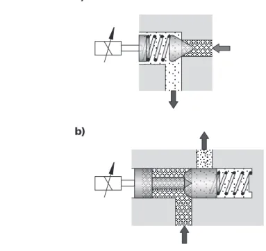
Actuation of pressure, flow control and directional control valves

In pressure valves, the spring is fitted between the proportional so-lenoid and the control cone (fig 2.3a).

■ With a reduced electrical current, the spring is only slightly

preten-sioned and the valve readily opens with a low pressure.

■ The higher the electrical current set through the proportional

so-lenoid, the greater the force applied on the armature. This moves to the right and the pretensioning of the spring is increased. The pres-sure, at which the valve opens, increases in proportion to the pre-tension force, i.e. in proportion to the armature position and the electrical current.

In flow control and directional control valves, the control spool is fit-ted between the proportional solenoid and the spring (fig. 2.3b).

■ In the case of reduced electrical current, the spring is only slightly

compressed. The spool is fully to the left and the valve is closed.

■ With increasing current through the proportional solenoid, the spool

is pushed to the right and the valve opening and flow rate increase.

a)

b)

Fig. 2.3 Actuation of a pressure and a restrictor valve

B-20

Positional control of the armature

Magnetising effects, friction and flow forces impair the performance of the proportional valve. This leads to the position of the armature not being exactly proportional to the electrical current.

A considerable improvement in accuracy may be obtained by means of closed-loop control of the armature position (fig. 2.4).

■ The position of the armature is measured by means of an inductive

measuring system.

■ The measuring signal x is compared with input signal y.

■ The difference between input signal y and measuring signal x is

amplified.

■ An electrical current I is generated, which acts on the proportional

solenoid.

■ The proportional solenoid creates a force, which changes the

posi-tion of the armature in such a way that the difference between input signal y and measuring signal x is reduced.

The proportional solenoid and the positional transducer form a unit, which is flanged onto the valve.

y-x I y U x Displacement encoder Comparator Amplifier Setpoint value I Fig. 2.4 Design of a position-controlled proportional solenoid

B-21

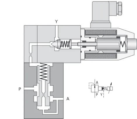
With a proportional pressure valve, the pressure in a hydraulic system can be adjusted via an electrical signal.

2.2 Design and mode of operation of proportional pressure valves

Pressure relief valve

Fig. 2.5 illustrates a pilot actuated pressure relief valve consisting of a preliminary stage with a poppet valve and a main stage with a control spool. The pressure at port P acts on the pilot control cone via the hole in the control spool. The proportional solenoid exerts the electrically adjustable counterforce.

■ The preliminary stage remains closed, if the force of the proportional

solenoid is greater than the force produced by the pressure at port P. The spring holds the control spool of the main stage in the lower position; flow is zero.

■ If the force exerted by the pressure exceeds the sealing force of the

pilot control cone, then this opens. A reduced flow rate takes place to the tank return from port P via port Y. The flow causes a pres-sure drop via the flow control within the control spool, whereby the pressure on the upper side of the control spool becomes less than the pressure on the lower side. The differential pressure causes a resulting force. The control spool travels upwards until the reset spring compensates this force. The control edge of the main stage opens so that port P and T are connected. The pressure fluid drains to the tank via port T.

B-22

P T P T Y Y Fig. 2.5 Pilot actuated proportional pressure relief valve

B-23

Pressure control valve

Fig. 2.6 iillustrates a pilot actuated 2-way pressure control valve. The pilot stage is effected in the form of a poppet valve and the main stage as a control spool. The pressure at consuming port A acts on the pilot control cone via the hole in the control spool. The counter force is set via the proportional solenoid.

■ If the pressure at port A is below the preset value, the pilot control

remains closed. The pressure on both sides of the control spool is identical. The spring presses the control spool downwards and the control edge of the main stage is open. The pressure fluid is able to pass unrestricted from port P to port A.

■ If pressure at port A exceeds the preset value, the pilot stage opens

so that a reduced flow passes to port Y. The pressure drops via the flow control in the control spool. The force on the upper side of the control spool drops and the control spool moves upwards. The cross section of the opening is reduced. As a result of this, the flow resistance of the control edge between port P and port A increases. Pressure a port A drops.

P A Y A P Y Fig. 2.6 Pilot actuated proportional pressure control valve

B-24

Proportional flow control valve

In the case of a proportional flow control valve in a hydraulic system, the throttle cross section is electrically adjusted in order to change the flow rate.

A proportional flow control valve is similarly constructed to a swit-ching 2/2-way valve or a switswit-ching 4/2-way valve.

2.3 Design and mode of operation of proportional flow control and directional control valves

With a directly actuated proportional flow control valve (fig. 2.7), the proportional solenoid acts directly on the control spool.

■ With reduced current through the proportional solenoid, both control

edges are closed.

■ The higher the electrical current through the proportional solenoid,

the greater the force on the spool. The spool moves to the right and opens the control edges.

The current through the solenoid and the deflection of the spool are proportional. P T A B P T B A Fig. 2.7

Directly actuated propor-tional restrictor valve without position control

B-25

Directly actuated proportional directional control valve

A proportional directional control valve ressembles a switching 4/3-way valve in design and combines two functions:

■ Electrically adjustable flow control (same as a proportional flow

con-trol valve),

■ Connection of each consuming port either with P or with T (same

as a switching 4/3-way valve).

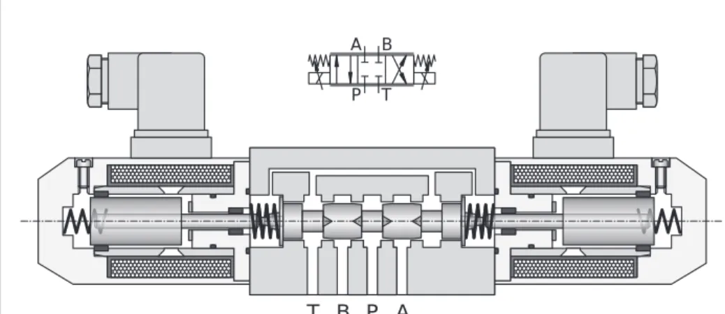
Fig 2.8 illustrates a directly actuated proportional directional control valve.

■ If the electrical signal equals zero, then both solenoids are

de-ener-gised. The spool is centred via the springs. All control edges are closed.

■ If the valve is actuated via a negative voltage, the current flows

through the righthand solenoid. The spool travels to the left. Ports P and B as well as A and T are connected together. The current through the solenoid and the deflection of the spool are proportional.

■ With a positive voltage, the current flows through the lefthand

so-lenoid. The spool moves to the right. Ports P and A as well as B and T are connected together. In this operational status too, the electrical current and the deflection of the spool are proportional to one another.

In the event of power failure, the spool moves to the mid-position so that all control edges are closed. (fail-safe position).

T B P A P T B A Fig. 2.8 Directly actuated proportional directional con-trol valve without

B-26

Pilot actuated proportional directional control valve

Fig. 2.9 shows a pilot actuated proportional directional control valve. A 4/3-way proportional valve is used for pilot control. This valve is used to vary the pressure on the front surfaces of the control spool, whereby the control spool of the main stage is deflected and the control edges opened. Both stages in the valve shown here are posi-tion controlled in order to obtain greater accuracy.

In the event of power or hydraulic energy failure, the control spool of the main stage moves to the mid-position and all control edges are closed (fail-safe position).

Two 3-way pressure regulators may be used for pilot control instead of a 4/3-way valve. Each pressure valve controls the pressure on one front surface of the main stage control spool.

C1 T A P B X C2 Y U S U S X P A Y T B C1 C2 Fig. 2.9 Pilot actuated

proportional directional control valve

B-27

Advantages and disadvantages of pilot actuated proportional valves

The force for the actuation of the main stage is generated hydrauli-cally in the pilot actuated valve. Only the minimal actuating force for the initial stage has to be generated by the proportional solenoid. The advantage of this is that a high level of hydraulic power can be controlled with a small proportional solenoid and a minimum of elec-trical current. The disadvantage is the additional oil and power con-sumption of the pilot control.

Proportional directional control valves up to nominal width 10 are pri-marily designed for direction actuation. In the case of valves with greater nominal width, the preferred design is pilot control. Valves with very large nominal width for exceptional flow rates may have three or four stages.

With proportional flow control and directional control valves, the flow rate depends on two influencing factors:

2.4 Design and mode of operation of proportional flow control valves

■ the opening of the control edge specified via the control signal, ■ the pressure drop via the valve.

To ensure that the flow is only affected by the control signal, the pressure drop via the control edge must be maintained constant. This is achieved by means of an additional pressure balance and can be realised in a variety of ways:

■ Pressure balance and control edge are combined in one flow control

valve.

■ The two components are combined by means of connection

techno-logy.

Fig. 2.10 shows a section through a 3-way proportional flow control valve. The proportional solenoid acts on the lefthand spool. The higher the electrical current through the proportional solenoid is set, the more control edge A-T opens and the greater the flow rate. The righthand spool is designed as a pressure balance. The pressure at port A acts on the lefthand side of the spool and the spring force and the pressure at port T on the righthand side.

B-28

■ If the flow rate through the valve is too great, the pressure drop on

the control edge rises, i.e. the differential pressure A-T. The control spool of the pressure balance moves to the right and reduces the flow rate at control edge T-B. This results in the desired reduction of flow between A and B.

■ If the flow rate is too low, the pressure drop at the control edge falls

and the control spool of the pressure balance moves to the left. The flow rate at control edge T-B rises and the flow increases.

In this way, flow A-B is independent of pressure fluctuations at both ports.

If port P is closed, the valve operates as a 2-way flow control valve. If port P is connected to the tank, the valve operates as a 3-way flow control valve.

T A P B T U B A P S Fig. 2.10 Proportional flow control valve

B-29

Proportional valves differ with regard to the type of valve, the control and the design of the proportional solenoid (table 2.1). Each combi-nation from table 2.1 results in one valve design, e.g.

2.5 Proportional valve designs: overview

■ a directly actuated 2/2-way proportional flow control valve without

positional control,

■ a pilot actuated 4/3-way proportional valve with positional control, ■ a directly actuated 2-way proportional flow control valve with

posi-tional control.

Valve types - Pressure valves Pressure relief valve 2-way pressure regulator 3-way pressure regulator - Restrictor valves 4/2-way restrictor

2/2-way restrictor valve - Directional control

valves 4/3-way valve 3/3-way valve

- Flow control valves 2-way flow control valve 3-way flow control valve Control type - directly actuated

- pilot actuated

Proportional solenoid - without position control - position controlled Table 2.1

Criteria for proportional valves

B-30

Chapter 3

Proportional valves:

Characteristic curves and parameters

B-31

B-32

Table 3.1 provides an overview of proportional valves and variables in a hydraulic system controlled by means of proportional valves.

3.1 Characteristic curve representation

The correlation between the input signal (electrical current) and the output signal (pressure, opening, flow direction or flow rate) can be represented in graphic form, whereby the signals are entered in a diagram:

■ the input signal in X-direction, ■ the output signal in Y-direction.

In the case of proportional behaviour, the characteristic curve is linear (fig. 3.1). The characteristic curves of ordinary valves deviate from this behaviour.

Valve types Input variable Output variable Pressure valve electr. current Pressure Restrictor valve electr. current Valve opening,

Flow (pressure-dependent) Directional control valve electr. current

Valve opening Flow direction Flow (pressure dependent) Flow control valve electr. current Flow (pressure

independent)

Table 3.1

Proportional valves: Input and

output variables

Input variable Output variable Current I Pressure p Proportional-pressure relief valve Y P T Pressure p Current I Output variable Input variable Fig. 3.1 Characteristic of a proportional pressure relief valve

B-33

Deviations from ideal behaviour occur as a result of spool friction and the magnetising effects, such as:

3.2 Hysteresis, inversion range and response threshold

■ the response threshold, ■ the inversion range, ■ the hysteresis.

Response threshold

If the electrical current through the proportional solenoid is increased, the armature of the proportional solenoid moves. As soon as the cur-rent ceases to change (fig. 3.2a), the armature remains stationary. The current must then be increased by a minimum amount, before the armature moves again. The required minimum variation is known as the response threshold or response sensitivity, which also occurs if the current is reduced and the armature moves in the other direc-tion.

Inversion range

If the input signal is first changed in the positive and then in the negative direction, this results in two separate branch characteristics, see diagram (fig. 3.2b). The distance of the two branches is known as the inversion range. The same inversion range results, if the cur-rent is first of all changed in the negative and then in the positive direction.

Hysteresis

If the current is changed to and fro across the entire correcting range, this results in the maximum distance between the branch characteristics. The largest distance between the two branches is known as hysteresis (fig. 3.2c).

The values of the response threshold, inversion range and hysteresis are reduced by means of positional control. Typical values for these three variables are around

■ 3 to 6% of the correcting range for unregulated valves

■ 0.2 to1% of the correcting range for position controlled valves

Sample calculation for a flow control valve without positional control: Hysteresis: 5% of correcting range,

Correcting range: 0...10 V

Distance of branch characteristics = (10 V - 0 V) 5% = 0.5 V

B-34

Output signal Output signal Output signal b) Inversion range c) Hysteresis a) Response threshold Input signal Input signal Input signal U H A Fig. 3.2 Response threshold, inversion range and hysteresis

B-35

The behaviour of the pressure valves is described by the pressure/ signal function. The following are plotted:

3.3 Characteristic curves of pressure valves

■ the electrical current in X-direction

■ the pressure at the output of the valve in Y-direction.

With flow control and directional control valves the deflection of the spool is proportional to the electrical current through the solenoid (fig. 2.7). 3.4 Characteristic curves of flow control and directional control valves Flow/signal function

A measuring circuit to determine the flow/signal function is shown in fig. 3.4. When recording measurements, the pressure drop above the valve is maintained constant. The following are plotted

■ the current actuating the proportional solenoid in X-direction, ■ the flow through the valve in Y-direction.

30

B-36

The flow rises not only with an increase in current through the so-lenoid, but also with an increase in pressure drop above the valve. This is why the differential pressure at which the measurement has been conducted is specified in the data sheets. Typical is a pressure drop of 5 bar, 8 bar or 35 bar per control edge.

Additional variables influencing the flow/signal function are

■ the overlap,

■ the shape of the control edges.

∆p q p2 p1 Fig. 3.4 Measurement of flow/ signal function

B-37

Overlap

The overlap of the control edges influences the flow/signal function. Fig. 3.5 clarifies the correlation between overlap and flow/signal func-tion using the examples of a proporfunc-tional direcfunc-tional control valve:

■ In the case of positive overlap, a reduced electrical current causes

a deflection of the control spool, but the flow rate remains zero. This results in a dead zone in the flow/signal function.

■ In the case of zero overlap, the flow/signal function in the low-level

signal range is linear.

■ In the case of negative overlap, the flow/signal function in the small

valve opening range results in a greater shape.

> 0 = 0 < 0 x x x x x x qB qB qB qA qA qA qL qL qL Fig. 3.5 Overlap and Flow/signal function

B-38

In practice, proportional valves generally have a positive overlap. This is useful for the following reasons:

■ The leakage in the valve is considerably less in the case of a spool

mid-position than with a zero or negative overlap.

■ In the event of power failure, the control spool is moved into

mid-position by the spring force (fail-safe mid-position). Only with positive overlap does the valve meet the requirement of closing the consu-ming ports in this position.

■ The requirements for the finishing accuracy of a control spools and

housing are less stringent than that for zero overlap.

Control edge dimensions

The control edges of the valve spool can be of different form. The following vary (fig. 3.6):

■ shapes of control edges,

■ the number of openings on the periphery, ■ the spool body (solid or drilled sleeve).

The drilled sleeve is the easiest and most cost effective to produce.

Fig. 3.6

Spool with different control edge patterns

B-39

Very frequently used is the triangular shaped control edge. Its advan-tages can be clarified on a manually operated directional control valve:

■ With a closed valve, leakage is minimal due to the overlap and the

triangular shaped openings.

■ Within the range of small openings, lever movements merely

pro-duce slight flow variations. Flow rate in this range can be controlled with a very high degree of sensitivity.

■ Within the range of large openings, large flow variations are

achieved with small lever deflections.

■ If the lever is moved up to the stop, a large valve opening is

ob-tained; consequently a connected hydraulic drive reaches a high velocity.

Similar to the hand lever, a proportional solenoid also permits con-tinuous valve adjustment. All the advantages of the triangular type control edges therefore also apply for the electrically actuated propor-tional valve. B A T B P A Precision controllability Piston deflection

Volumetric flow rate q

Manual lever path

A B B A Piston overlap Fig. 3.7

Manually operated valve with triangular control edge

B-40

Fig. 3.8 illustrates the flow/signal function for two different types of control edge:

■ With reduced electrical current, both control edges remain closed

due to the positive overlap.

■ The rectangular control edge causes a practically linear pattern of

the characteristic curve.

■ The triangular control edge results in a parabolic flow/signal

func-tion. 8 8 l/min l/min 4 4 2 2 100 100 300 300 700 700 mA mA 0 0 q q I I Fig. 3.8

Flow/signal functions for two different spool patterns

B-41

Many applications require proportional valves, which are not only able to follow the changes of the electrical input accurately, but also very quickly. The speed of reaction of a proportional valve can be speci-fied by means of two characteristic values:

3.5 Parameters of valve dynamics

1. Manipulating time:

designates the time required by the valve to react to a change in the correcting variable. Fast valves have a small manipulating time.

2. Critical frequency:

indicates how many signal changes per second the valve is able to follow. Fast valves demonstrate a high critical frequency.

Manipulating time

The manipulating time of a proportional valve is determined as fol-lows:

■ The control signal is changed by means of a step change.

■ The time required by the valve to reach the new output variable is

measured.

The manipulating time increases with large signal changes (fig. 3.9). Moreover, a large number of valves have a different manipulating time for positive and negative control signal changes.

The manipulating times of proportional valves are between approx. 10 ms (fast valve, small control signal change) and approx. 100 ms (slow valve, large control signal change).

B-42

Frequency response measurement

In order to be able to specify the critical frequency of a valve, it is first necessary to measure the frequency response.

To measure the frequency response, the valve is actuated via a sin-usoidal control signal. The correcting variable and the spool position are represented graphically by means of an oscilloscope. The valve spool oscillates with the same frequency as the control signal (fig. 3.10).

If the actuating frequency is increased whilst the activating amplitude remains the same, then the frequency with which the spool oscillates also increases. With very high frequencies, the spool is no longer able to follow the control signal changes. The amplitude A2 in fig. 3.10e is clearly smaller than the amplitude A1 in fig. 3.10d.

0

20

40

60

%

100

0

10

20

ms

30

(Proportional directional control valve)

B-43

The frequency response of a valve consists of two diagrams:

■ the amplitude response, ■ the phase response.

b) d) e) c) A1 _A2 xs Y Critical frequency Spo ol position Control signal y y xs xs a) Measuring circuit

Function generator Oscilloscope

y Low frequency Time t Time t Time t Time t Fig. 3.10: Measurement of frequency response with a proportional directional control valve

B-44

Amplitude response

The ratio of the amplitude at measured frequencies to the amplitude at very low frequencies is specified in dB and plotted in logarithmic scale. An amplitude ratio of -20 dB means that the amplitude has dropped to a tenth of the amplitude at low frequency. If the ampli-tude for all measured values is plotted against the measured fre-quency, this produces the amplitude response (fig. 3.11).

Phase response

The delay of the output signal with regard to the input signal is spe-cified in degrees. A 360 degree phase displacement means that the output signal lags behind the input signal by an entire cycle. If all the phase values are plotted against the measuring frequency, this re-sults in the phase response (fig. 3.11).

Frequency response and control signal amplitude

With a 10% correcting variable amplitude (= 1 volt), the control spool only needs to cover a small distance. Consequently, the control spool is also able to follow signal changes with a high frequency. Ampli-tude and phase response only inflect with a high frequency from the horizontal (fig. 3.11).

With a 90% correcting variable amplitude ( = 9 Volt), the required distance is nine times as great. Accordingly, it is more difficult for the control spool to follow the control signal changes. Amplitudes and phase response already inflect at a low frequency from the horizontal (fig. 3.11).

Critical frequency

The critical frequency is read from the amplitude response. It is the frequency, at which the amplitude response has dropped to 70.7% or -3 dB.

The frequency response (fig. 3.11) results in a critical frequency of approx.. 65 Hertz at 10% of the maximum possible control signal am-plitude. For 90% control signal amplitude the critical frequency is at approx. 23 Hertz.

The critical frequencies of proportional valves are between approx. 5 Hertz (slow valve, large control signal amplitude) and approx. 100 Hertz (fast valve, small control signal amplitude).

B-45

The application limits of a proportional valve are determined by

3.6 Application limits of propor-tional valves

■ the pressure strength of the valve housing,

■ the maximum permissible flow force applied to the valve spool.

If the flow force becomes to great, the force of the proportional so-lenoid is not sufficient to hold the valve spool in the required position. As a result of this, the valve assumes an undefined status.

The application limits are specified by the manufacturer either in the form of numerical values for pressure and flow rate or in the form of a diagram.

-2

-4

-6

0

+2

dB

Amplitude

ratio A/A

Phase shif

t

ϕ

-8

-10°

± 10%

± 10%

± 25%

± 90%

± 90%

± 25%

5

5

10

10

20

20

50

50

30

30

200

200

100

100

Hz

Hz

-30°

-50°

-70°

-90°

Frequency f

Frequency f

B-46

Chapter 4

Amplifier and

setpoint value specification

B-47

B-48

The control signal for a proportional valve is generated via an elec-tronic circuit. Fig. 4.1 illustrates the signal flow between the control and proportional solenoid. Differentiation can be made between two functions:

■ Setpoint value specification:

The correcting variable (= setpoint value) is generated electronically. The control signal is output in the form of an electrical voltage. Since only a minimal current flows, the proportional solenoid cannot be directly actuated.

■ Amplifier:

The electrical amplifier converts the electrical voltage in the form of an input signal into a electrical current in the form of an output signal. It provides the electrical power required for the valve actua-tion. Setpoint value specification Amplifier Proportional solenoid Voltage V Current I Fig. 4.1

Signal flow between controller and proportional solenoid (schematic)

B-49

Modules

The setpoint value specification and amplifier can be grouped into electronic modules (electronic cards) in various forms. Three ex-amples are illustrated in fig. 4.2 .

■ A control system, which can only process binary signals is used

(e.g. simple PLCs). Setpoint value specification and amplifier consti-tute separate modules (fig. 4.2a).

■ A PLC with analogue outputs is used. The correcting variable is

directly generated, including special functions such as ramp genera-tion and quadrant recognigenera-tion. No separate electronics are required for the setpoint value specification (fig. 4.2b).

■ Mixed forms are frequently used. If the control is only able to specify

constant voltage values, additional functions such as ramp genera-tion are integrated in the amplifier module (fig. 4.2c).

Setpoint value specification Setpoint value processing Controller Controller Controller Amplifier Amplifier Amplifier Proportional solenoid Proportional solenoid Proportional solenoid Binary signals a) b) c) Voltage V Voltage V Voltage V Current I Current I Current I Fig. 4.2 Electronic modules for signal flow between controller and proportional solenoid

B-50

With amplifiers for proportional valves, differentiation is made between to designs:

4.1 Design and mode of operation of an amplifier

■ The valve amplifier is built into the valve

(integrated electronics)

■ The valve amplifier is designed in the form of separate module or

card (fig. 1.6).

Amplifier functions

Fig. 4.3a illustrates the three major functions of a proportional valve amplifier:

■ Correcting element:

The purpose of this is to compensate the dead zone of the valve (see chapter. 4.2).

■ Pulse width modulator:

This is used to convert the signal (= modulation).

■ End stage:

This provides the required electrical capacity.

For valves with position controlled proportional solenoids, the sensor evaluation and the electronic closed-loop control are integrated in the amplifier (fig. 4.3b). The following additional functions are required:

■ Voltage source:

This generates the supply voltage of the inductive measuring sys-tem.

■ Demodulator:

The demodulator converts the voltage supplied by measuring sys-tem.

■ Closed-loop controller:

In the closed-loop controller, a comparison is made between the prepared correcting variables and the position of the armature. The input signal for the pulse width modulation is generated according to the result.

B-51

One and two-channel amplifier

A one-channel amplifier is adequate for valves with one proportional solenoid. Directional control valves actuated via two solenoids, require a two-channel amplifier. Depending on the control signal status, cur-rent is applied either to the lefthand or to the righthand solenoid only.

Setpoint value V

b) with positional control of the armature a) without positional control of the armature

Correction V V Current I Pulse width modulation End stage Setpoint value V Armature position V Correction Demodulator V V V Current I Voltage supply V Closed-loop controller Pulse width

modulation End stage

Voltage supply for displacement encoder

Fig. 4.3 Block diagrams for one-channel amplifier

B-52

Pulse width modulation

Fig 4.5 illustrates the principle of pulse width modulation. The electri-cal voltage is converted into pulses. Approximately ten thousand pul-ses per second are generated.

When the end stage has been executed, the pulse-shaped signal acts on the proportional solenoid. Since the proportional solenoid coil inductivity is high, the current cannot change as rapidly as the electri-cal voltage. The current fluctuates only slightly by a mean value.

■ A small electrical voltage as an input signal creates small pulses.

The average current of the solenoid coil is small.

■ The greater the electrical voltage, the wider the pulse. The average

current through the solenoid coil increases.

The average current through the solenoid and the input voltage of the amplifier are proportional to one another.

V Setpoint value V Correction V V V V Current I Current I Sign recognition Pulse width modulation End stages Fig. 4.4 Two-channel amplifier (without positional control of armature)

B-53

Dither effect

The slight pulsating of the current as a result of the pulse width mo-dulation causes the armature and valve spool to perform small oscil-lations at a high frequency. No static friction occurs. The response threshold, inversion range and hysteresis of the valve are clearly re-duced.

The reduction in friction and hysteresis as a result of a high frequen-cy signal is known as dither effect. Certain amplifiers permit the user to create an additional dither signal irrespective of pulse width modu-lation.

Heating of amplifier

As a result of pulse width modulation, three switching stages occur in end stage transistors:

■ Lower signal value:

The transistor is inhibited. The power loss in the transistor is zero, since no current flows.

■ Upper signal value:

The transistor is conductive. The transistor resistance in this status is very small and only a very slight power loss occurs.

■ Signal edges:

The transistor switches over. Since the switch-over is very fast, power loss is very slight.

Overall, the power loss is considerably less than with an amplifier without pulse width modulation. The electronic components become less heated and the construction of the amplifier is more compact.

B-54

Ieff Ieff Solenoid voltage V Solenoid voltage V Solenoid voltage V T = Duty cycle T T Time t Time t Time t 24 V 24 V 24 V 0 0 0 Ieff = Effective magnetising current Fig. 4.5

Pulse width modulation

B-55

Dead zone compensation 4.2 Setting an

amplifier

Fig. 4.6a illustrates the flow/signal characteristic for a valve with posi-tive overlap. As a result of the overlap, the valves has a marked dead zone.

If you combine a valve and an amplifier with linear characteristic, , the dead zone is maintained (fig. 4.6b).

If an amplifier is used with a linear characteristic as in fig. 4.6c, the dead zone can be compensated against this.

+ -Current I Flow rate q P A A → Flow rate q P B B → Solenoid 2 actuated Solenoid 1 actuated V V V V Amplifier Amplifier I I q q q q Valve Valve Amplifier and valve Amplifier and valve b) a) c) I I q q q q V V I I V V P T B Y2 Y1 A Fig. 4.6 Compensating dead zone with a

B-56

Setting the amplifier characteristic

The valve amplifier characteristic can be set, whereby it is possible to

■ use the same amplifier type for different valve types, ■ compensate manufacturing tolerances within a valve series,

■ replace only the valve or only the amplifier in the event of a fault.

The amplifier characteristic exhibits the same characteristics for valves by different manufacturers. However, the characteristic values are in some cases designated differently by various manufacturers and, accordingly, the setting instructions also vary.

Fig. 4.7 represents an amplifier characteristic for a two-channel ampli-fier. Solenoid 1 only is supplied with current for a positive control signal, and solenoid 2 only for a negative control signal.

Three variables are set:

■ Maximum current

The maximum current can be adjusted in order to adapt the ampli-fier to proportional solenoids with different maximum current. With certain amplifiers, an amplification factor is set instead of the maxi-mum current, which specifies the slope of the amplifier charac-teristic.

■ Jump current

The jump current can be adjusted in order to compensate different overlaps. With various manufacturers, the jump current is set via a “signal characteriser”.

■ Basic current

Due to manufacturing tolerances, the valve spool may not be exactly in the mid-position when both solenoids are de-energised. This error can be compensated by means of applying a basic current to one of the two proportional solenoids. The level of the basic current can be set. The term “offset setting” is often used to describe this com-pensating measure.

B-57

Correcting variable V Maximum current 1 Maximum current 2 Current I2 Current I1 Jump current Basic current l0 Jump current Vmin Vmax Fig. 4.7 Setting options with a two channel valve amplifier

B-58

An electrical voltage is required as a control signal (= setpoint value) for a proportional valve. The voltage can generally be varied within the following ranges:

4.3 Setpoint value specification

■ between 0 V and 10 V for pressure and restrictor valves, ■ between -10 V and 10 V for directional control valves.

The correcting variable y can be generated in different ways. Two examples are shown in (fig. 4.8).

■ The potentiometer slide is moved by means of a hand lever. The

correcting variable is tapped via the slide; this facilitates the remote adjustment of valves (fig. 4.8a).

■ A PLC is used for the changeover between two setpoint values set

by means of potentiometers (fig. 4.8b).

10V

24V 10V

0V

Setpoint value card 0V y y PLC K K a) b) Fig. 4.8

Examples for setpoint value specification

a) Hand lever

b) Reversal via a PLC

B-59

Avoidance of pressure peaks and vibrations

Vibrations and pressure points are caused as a result of reversing a directional control valve. Fig 4.9 compares three reversing variants. A switching directional control valve only has the settings “valve open” and “valve closed". A change in the control signals leads to sudden pressure changes resulting in jerky acceleration and vibrati-ons of the drive (fig. 4.9a).

With a proportional valve, it is possible to set different valve openings and speeds. With this circuit too, sudden changes in the control signal causes jerky acceleration and vibrations (fig. 4.9b).

To achieve a smooth, regular motion sequence, the correcting vari-able of the proportional valve is changed to a ramp form (fig. 4.9c).

B-60

t t t t t t t Y1 y y Y2 v v v a) b) c) v v v P P P T T T B B B A A A Y2 Y2 Y2 Y1 Y1 Y1

m

m

m

Setpoint value specifica-tion and velocity of a cylinder drive

B-61

Different ramp slopes are frequently required for the retracting and advancing of a cylinder. Moreover, many applications also require dif-ferent ramp slopes for the acceleration and deceleration of loads. For such applications, ramp shapers are used, which automatically recog-nise the operational status and changeover between different ramps. Fig. 4.10 illustrates an application for various ramp slopes: a cylinder with unequal piston areas moving a load in the vertical direction.

Ramp shapers can be realised in different ways:

■ built into the valve amplifier,

■ with separate electronics connected between the controller and the

valve amplifier,

■ by means of programming a PLC with analogue outputs.

Phase 1 Phase 2 t y α2 α3 α4 α1 Phase 1 Phase 2 P T B A Y2 Y1

m

B-62

Chapter 5

Switching examples with

proportional valves

B-63

B-64

Flow characteristics of proportional restrictors and directional control valves

5.1 Speed control

The flow rate across the control edge of a proportional valve de-pends on the pressure drop. The following correlation applies be-tween pressure drop and flow rate if the valve opening remains the same:

This means: If the pressure drop across the valve is doubled, the flow range increases by factor , i.e. to 141.4%.

Load-dependent speed control with proportional directional control valves

In the case of a hydraulic cylinder drive, the pressure drop across the proportional directional control valve falls, if the drive has to oper-ate against force. Because of the pressure-dependency of the flow, the traversing speed also drops. This is to be explained by means of an example.

Let us consider the upwards movement of a hydraulic cylinder drive for two load cases:

■ without load (fig. 5.1a), ■ with load (fig. 5.1b).

The correcting variable is 4 V in both cases, i.e.: The valve opening is identical.

Without load, the pressure drop across each control edge of the pro-portonal directional control valve is 40 bar. The piston of the drive moves upwards with speed v = 0.2 m/s (fig. 5.1a).

q ~ ∆p

2

B-65

If the cylinder has to lift a load, the pressure increases in the lower chamber, whilst the pressure in the upper chamber drops. Both these effects cause the pressure drop across the valve control edges to reduce, i.e. to 0 bar per control edge in the example shown.

The flow rate is calculated as follows:

Speed and flow are proportional to one another. Consequently, the speed in the loaded state is calculated as follows:

The speed is therefore considerably less than that without load de-spite identical valve opening.

q q p p with load without load with load without load = ∆ = = ∆ 1 4 1 2 q v v v q q v v m s with load without load with load without load with load without load

~ . / = = = = 1 2 1 2 0 1

B-66

a) b) t t y v 4V 0.2 m/s t t y v 4V 0.1 m/s p = 40 barB p = 50 barA p = 90 bar0 ∆p = 40 bar ∆p = 40 bar P T B A v Y2 Y1 p = 10 barB p = 80 barA p = 90 bar0 ∆p = 10 bar ∆p = 10 bar P T B A v Y2 Y1 m Fig. 5.1 Velocity of a

valve actuated cylinder drive for two types of load a) without load

b) with load

B-67

Load-independent speed control with proportional directional control valve and pressure balance

An additional pressure balance causes the pressure drop across the proportional directional control valve to remain constant irrespective of load. Flow and speed become load independent.

Fig 5.2 represents a circuit with feed pressure balance. The shuttle valve ensures that the higher of the two chamber pressures is al-ways supplied to the pressure balance.

B P T A Y2 Y1 Fig. 5.2 Valve actuated cylinder drive with supply pressure balance

B-68

Differential circuit

With machine tools, two tasks are frequently required from hydraulic drives:

■ fast feed speed for rapid traverse,

■ high force and accurate, constant speed during working step.

Both requirements can be met by using the circuit shown in fig. 5.3.

■ Extending the piston in rapid traverse causes the restrictor valve to

open. The pressure fluid flows from the piston annular side through both valves to the piston side; the piston reaches a high speed.

■ Extending the piston during the working step causes the restrictor

valve to close. The pressure on the annular surface drops and the drive is able to exert a high force.

■ Since the restrictor valve is in the form of a proportional valve, it is

possible to changeover smoothly between rapid traverse and a working step.

■ The restrictor valve remains closed during the return stroke.

Special 4/3-way proportional valves combining the functions of both valves are also used for differential circuits.

P T B A Y2 Y1 A P Y3 Fig 5.3 Differential circuit

B-69

Counter pressure

When decelerating loads, the pressure in the relieved cylinder cham-ber may drop below the ambient pressure. Air bubbles may be crea-ted in the oil as a result of the low pressure and the hydraulic sys-tem may be damaged due to cavitation.

The remedy for this is counter pressure via a pressure relief valve. This measure results in a higher pressure in both chambers and cavitation is eliminated.

The pressure relief valve is additionally pressurised with the pressure from the other cylinder chamber. This measure causes the opening of the pressure relief valve when the load is accelerated, thereby preventing the counter pressure having any detrimental in this opera-tional status. P T B A Y2 Y1 m Fig. 5.4 Counter pressure with pressure relief valve

B-70

Proportional restrictors and proportional directional control valves are available in the form of spool valves. With spool valves, a slight leak-age occurs in the mid-position, which leads to slow “cylinder creedp” with a loaded drive. It is absolutely essential to prevent this gradual creep in many applications, e.g. lifts.

In the case of an application, where the load must be maintained free of leakage, the proportional valve is combined with a poppet valve. Fig. 5.5 illustrates a circuit with proportional directional control valve and a piloted, (delockable) non-return valve.

5.2 Leakage prevention

Positioning drives are always used in those applications where loads have to be moved fast and accurately to a specific location. A lift is a typical example of an application for a hydraulic positioning drive. Cost-effective hydraulic positioning drives may be realised using pro-portional directional control valves and proximity sensors.

Fig. 5.6a shows a circuit using a proximity sensor. Initially, the drive moves at a high speed owing to the large valve opening. After pas-sing the sensor, the valve opening is reduced (ramp-shaper) and the drive decelerated. If the load is increased, this may lead to a distinct extension of the deceleration path and overtravelling of the destina-tion posidestina-tion (fig. 5.6a)

5.3 Positioning P T B B X A A Y2 Y1

m

Retention of a load using a piloted non-return valve

B-71

Rapid traverse/creep speed circuit

A high positioning accuracy is obtained by means of a rapid tra-verse/creep speed circuit. After passing the first proximity sensor, the valve opening is reduced (ramp shaper) to a very small value. After passing the second proximity sensor, the valve is closed without ramp. Due to the reduced output speed for the second deceleration process, the position deviations for different loads are very slight (fig. 5.6b). a) b) Position x Position x small load small load large load large load x x1 x2 Velocity v Velocity v Rapid traverse Creep speed P T B A Y2 Y1

m

B-72

Hydraulic drives are mainly used in applications, where large loads are moved and high forces generated. The power consumption and costs of a system are correspondingly high, which leaves room for a considerable potential saving in energy and cost.

5.4 Energy saving measures

Initially any measures to save energy by means of circuit technology represent an increase in the construction costs of a hydraulic system. However, by reducing power consumption, the additional costs usual-ly can be very quickusual-ly recouped after a very short period of opera-tion.

When movements are controlled by means of proportional valves, pressure drops via the control edges of the proportional valve. This leads to loss of energy and heating of the pressure medium.

Additional losses of energy may occur because the pump creates a higher flow rate than that required for the movement of the drive. The superfluous flow is vented to the tank via the pressure relief valve without performing a useful task.

Figs. 5.7 to 5.10 illustrate different circuit variants for a cylinder drive controlled by means of a proportional directional control valve. The following are represented for each circuit variant:

■ the circuit diagram,

■ the drive speed as a function of time (identical for all circuits, since

the motion sequence of the drive is the same),

■ the absorbed power of the pump as a function of time.

B-73

Fixed displacement pump, mid-position of directional control valve: closed

Fig. 5.7 illustrates a circuit, where the fixed displacement pump and the proportional directional control valve with mid-position closed are combined. The pump must be designed for the maximum required flow rate, continually supply this flow rate and deliver against the sys-tem pressure. Consequently, the resulting power consumption is cor-respondingly high.

Fixed displacement pump, mid-position of directional control valve: Tank by-pass

A reduction in power consumption may be obtained by means of using a proportional valve with tank by-pass (fig. 5.8). Whilst the drive is stationary, the pump nevertheless supplies the full flow rate, but only needs to build up a reduced pressure, thus reducing the absorbed power during these phases accordingly. In the main, this leads to a lesser power consumption than that of the circuit shown in fig. 5.7. t t v P P T B A Y2 Y1 M Fig. 5.7 Power consumption of a fixed displacement pump (mid-position of directional control valve: closed) t t v P P T B A Y2 Y1 M Fig. 5.8 Power consumption of a fixed displacement pump (mid-position of

B-74

Fixed displacement pump with reservoir

In many cases, the use of a valve with tank by-pass it not possible, since the pressure in the cylinder drops as a result of this. In such a case, a reservoir may be used (fig. 5.9). If the drive does not move at all or only slowly, then the pump loads the reservoir. In the rapid movement phases, part of the flow is supplied by the reservoir, whereby a smaller pump with a reduced delivery rate can be used. This leads to a reduction in absorbed power and power consumption.

t t v P P T B A Y2 Y1 M Fig. 5.9 Power consumption of a fixed displacement pump with additional reservoir (mid-position of directional control valve: closed)

B-75

Variable displacement pump

The variable displacement pump is driven at a constant speed. The input volume (= delivered oil volume per pump revolution) is adjust-able, whereby the flow rate delivered by the pump is also changed. The variable displacement pump is adjusted with two cylinders:

■ The control cylinder with the larger piston area adjusts the pump in

relation to higher flow rates.

■ The control cylinder with the smaller piston area adjusts the pump

in relation to smaller flow rates.

Pump regulation (circuit fig. 5.10) operates as follows:

■ If the opening of the proportional directional control valve increases,

the pressure at the pump output decreases. The switching valve of the pump regulator opens. The pump is driven by the control cylin-der with the larger piston area and creates the required increased flow rate.

■ If the opening of the directional control valve is reduced, the

pres-sure rises at the pump output. Consequently, the 3/2-way valve switches. The control cylinder with the large piston area is connec-ted with the tank. The pump reverts to the smaller control cylinder, resulting in a reduction in the flow rate. The absorbed power of the pump drops.

■ With a closed valve, the flow rate and therefore the absorbed power

of the pump is reduced down to zero. The absorbed power of the pump reverts to a very small value, which is required to overcome the frictional torque.

B-76

The pressure relief valve is used merely for protection. The response pressure of this valve must be set higher than the working pressure of the pump. So long as the variable displacement pump operates fault-free, the valve remains closed.

If there is a sudden change in the valve opening, the pump cannot react sufficiently quickly. In this operating status a pressure reservoir is used as a buffer in order to prevent strong fluctuations in the supply pressure. Compared with the circuit shown in fig. 5.9 a low pressure reservoir is adequate.

Comparison of power consumption between a fixed and a variable displacement pump

In contrast with the fixed displacement pump, the variable capacity pump only generates the flow rate actually required by the drive. Power losses are therefore minimised. The circuit using the variable displacement pump therefore displays the lowest power consumption.

t t v P P T B A Y2 Y1 Fig. 5.10 Power consumption of a variable displacement pump (mid-position of directional control valve: closed)

B-77