The Relationship between Crude Oil and Natural Gas Prices

InstItute for PublIc PolIcy

r I c E u n I v E r s I t y

Natural Gas in North America:

Markets and Security

The Relationship between Crude Oil and Natural Gas

Prices

THE JAMES A.BAKER IIIINSTITUTE FOR PUBLIC POLICY

RICE UNIVERSITY

THE RELATIONSHIP BETWEEN CRUDE OIL AND

NATURAL GAS PRICES

By

P

H

,

P

.D.

GEORGE AND CYNTHIA MITCHELL CHAIR AND

PROFESSOR OF ECONOMICS,RICE UNIVERSITY,

RICE SCHOLAR,JAMES A.BAKER IIIINSTITUTE FOR PUBLIC POLICY

K

B.

M

III,

P

.D.

FELLOW IN ENERGY STUDIES,JAMES A.BAKER IIIINSTITUTE FOR PUBLIC POLICY, ADJUNCT ASSISTANT PROFESSOR OF ECONOMICS,RICE UNIVERSITY

AND

J

R

JAMES A.BAKER IIIINSTITUTE FOR PUBLIC POLICY, GRADUATE STUDENT,DEPARTMENT OF ECONOMICS,

RICE UNIVERSITY

PREPARED IN CONJUNCTION WITH AN ENERGY STUDY SPONSORED BY

THE JAMES A.BAKER IIIINSTITUTE FOR PUBLIC POLICY AND MCKINSEY &COMPANY

THIS PAPER WAS WRITTEN BY A RESEARCHER (OR RESEARCHERS) WHO PARTICIPATED IN A

BAKER INSTITUTE STUDY, “NATURAL GAS IN NORTH AMERICA: MARKETS AND SECURITY.”

WHEREVER FEASIBLE, THIS PAPER WAS REVIEWED BY OUTSIDE EXPERTS BEFORE THEY ARE RELEASED.HOWEVER, THE RESEARCH AND VIEWS EXPRESSED IN THESE PAPERS ARE THOSE OF THE INDIVIDUAL RESEARCHER(S) AND DO NOT NECESSARILY REPRESENT THE VIEWS OF THE

JAMES A.BAKER IIIINSTITUTE FOR PUBLIC POLICY.

©2007 BY THE JAMES A.BAKER IIIINSTITUTE FOR PUBLIC POLICY OF RICE UNIVERSITY

THIS MATERIAL MAY BE QUOTED OR REPRODUCED WITHOUT PRIOR PERMISSION, PROVIDED APPROPRIATE CREDIT IS GIVEN TO THE AUTHOR AND

ABOUT THE POLICY REPORT

N

ATURAL

G

AS IN

N

ORTH

A

MERICA

:

M

ARKETS AND

S

ECURITY

Predicted shortages in U.S. natural gas markets have prompted concern about the future of U.S. supply sources, both domestically and from abroad. The United States has a premier energy resource base, but it is a mature province that has reached peak production in many traditional producing regions. In recent years, environmental and land-use considerations have prompted the United States to remove significant acreage that was once available for exploration and energy development. Twenty years ago, nearly 75 percent of federal lands were available for private lease to oil and gas exploration companies. Since then, that share has fallen to 17 percent. At the same time, U.S. demand for natural gas is expected to grow close to 2.0 percent per year over the next two decades. With growth in domestic supplies of natural gas production in the lower 48 states expected to be constrained in the coming years, U.S. natural gas imports are expected to rise significantly in the next two decades, raising concerns about supply security and prompting questions about what is appropriate national natural gas policy.

The future development of the North American natural gas market will be highly influenced by U.S. policy choices and changes in international supply alternatives.

The Baker Institute Policy Report on Natural Gas in North America: Markets and Security brings together two research projects undertaken by the Baker Institute’s Energy Forum. The first study focuses on the future development of the North American natural gas market and the factors that will influence supply security and pricing. This study considers, in particular, how access to domestic resources and the growth of international trade in liquefied natural gas will impact U.S. energy security. The second study examines the price relationship between oil and natural gas, with special attention given to natural gas demand in the industrial and power generation sectors – sectors in which natural gas can be displaced by competition from other fuels. This policy report is

designed to help both market participants and policymakers understand the risks associated with various policy choices and market scenarios.

ACKNOWLEDGEMENTS

The James A. Baker III Institute for Public Policy would like to thank McKinsey & Company and the sponsors of the Baker Institute Energy Forum for their generous support in making this project possible.

The authors of this paper would also like to acknowledge the seminar participants at Rice University and the United States Association for Energy Economics annual meetings, 2006, Ann Arbor, Michigan, for valuable comments.

ABOUT THE AUTHORS

PETER HARTLEY,PH.D.

GEORGE AND CYNTHIA MITCHELL CHAIR ANDPROFESSOR OF ECONOMICS,RICE UNIVERSITY,

RICE SCHOLAR,JAMES A.BAKER IIIINSTITUTE FOR PUBLIC POLICY

Peter Hartley is the George and Cynthia Mitchell chair and a professor of economics at Rice University. He is also a Rice scholar of energy economics for the James A. Baker III Institute for Public Policy. He has worked for more than 25 years on energy economics issues, focusing originally on electricity, but including also work on gas, oil, coal, nuclear and renewables. He wrote on reform of the electricity supply industry in Australia throughout the 1980s and early 1990s and advised the government of Victoria when it completed the acclaimed privatization and reform of the electricity industry in that state in 1989. The Victorian reforms became the core of the wider deregulation and reform of the electricity and gas industries in Australia. Apart from energy and environmental economics, Hartley has published research on theoretical and applied issues in money and banking, business cycles and international finance. In 1974, he completed an honors degree at the Australian National University, majoring in mathematics. He worked for the Priorities Review Staff, and later the Economic Division, of the Prime Minister’s Department in the Australian government while completing a master’s degree in economics at the Australian National University in 1977. Hartley obtained a Ph.D. in economics at the University of Chicago in 1980.

KENNETH B.MEDLOCK III,PH.D.

FELLOW IN ENERGY STUDIES,JAMES A.BAKER IIIINSTITUTE FOR PUBLIC POLICY,

ADJUNCT ASSISTANT PROFESSOR OF ECONOMICS,RICE UNIVERSITY

Kenneth B. Medlock III is currently research fellow in energy studies at the James A. Baker III Institute for Public Policy and adjunct assistant professor in the department of economics at Rice University. He is a principal in the development of the Rice World Natural Gas Trade Model, which is aimed at assessing the future of liquefied natural gas

(LNG) trade. Medlock’s research covers a wide range of topics in energy economics, such as domestic and international natural gas markets, choice in electricity generation capacity and the importance of diversification, gasoline markets, emerging technologies in the transportation sector, modeling national oil company behavior, economic development and energy demand, forecasting energy demand, and energy use and the environment. His research has been published in numerous academic journals, book chapters and industry periodicals. For the department of economics, Medlock teaches courses in energy economics.

JENNIFER ROSTHAL

GRADUATE FELLOW,JAMES A.BAKER IIIINSTITUTE FOR PUBLIC POLICY,

GRADUATE STUDENT,DEPARTMENT OF ECONOMICS,RICE UNIVERSITY

Jennifer Rosthal is a graduate fellow at the James A. Baker III Institute for Public Policy Energy Forum and a Ph.D. student in the Rice University economics department. Rosthal's research focuses on United States natural gas and electricity demand and gas and petroleum product-price relationships. Prior to coming to Rice University, Rosthal worked as a research assistant at Hobart and William Smith Colleges and co-authored the book, “Pathways to a Hydrogen Future” (Elsevier Science, 2007). She has presented her work at the United States Association of Energy Economics (USAEE) conferences and holds the student representative position on the USAEE Council. Rosthal has a B.A. in economics from William Smith College.

ABOUT THE ENERGY FORUM AT THE

J

AMES

A.

B

AKER

III

I

NSTITUTE FOR

P

UBLIC

P

OLICY

The Baker Institute Energy Forum is a multifaceted center that promotes original, forward-looking discussion and research on the energy-related challenges facing our society in the 21st century. The mission of the Energy Forum is to promote the development of informed and realistic public policy choices in the energy area by educating policy makers and the public about important trends—both regional and global—that shape the nature of global energy markets and influence the quantity and security of vital supplies needed to fuel world economic growth and prosperity.

The forum is one of several major foreign policy programs at the James A. Baker III Institute for Public Policy at Rice University. The mission of the Baker Institute is to help bridge the gap between the theory and practice of public policy by drawing together experts from academia, government, the media, business, and nongovernmental organizations. By involving both policymakers and scholars, the institute seeks to improve the debate on selected public policy issues and make a difference in the formulation, implementation, and evaluation of public policy.

The James A. Baker III Institute for Public Policy Rice University – MS 40

P.O. Box 1892 Houston, TX 77251-1892 http://www.bakerinstitute.org

I. Introduction

The relationship between natural gas and crude oil prices affects energy consumers, producers and marketers. For example, energy prices for the two fuels influence the incentives to invest in inventories or different types of energy-using equipment. Energy market traders also are interested to know whether there is a tendency for the relative prices of different energy commodities to return to a particular value, since if such a tendency exists, it might form the basis of a trading strategy.

Historically, it was thought that the prices of West Texas Intermediate (WTI) crude oil and natural gas delivered at the Henry Hub, which are the most widely quoted energy prices in the United States, maintained a 10-1 relationship, so that one barrel of WTI crude oil priced at roughly 10 times 1 million British thermal units (MMBtu) of natural gas. More recently, this appears to have declined by about 40% to a 6-1 ratio, which is close to thermal parity. However, the observed variability in the relative price relationship has led some to question whether the natural gas price has decoupled from the crude oil price. In this paper, we investigate the existence of a long run stable relationship between crude oil and natural gas prices, identify shocks that cause departures from that relationship, and estimate the length of the adjustment process that re-establishes the long-term relationship between the prices of the two fuels.

Importantly, we conclude that U.S. natural gas and crude oil prices remain linked in their term movements. We demonstrate that the narrowing in the relative long-term price relationship between U.S. crude oil benchmark WTI and Henry Hub natural gas prices reflects the widespread adoption of combined cycle gas turbines (CCGT), which has increased the efficiency of using natural gas to generate electricity in place of oil-based fuel. In addition, we find that the ratio of the price of WTI crude to the price of natural gas at the Henry Hub will tend to remain about 40% lower than it would have been a decade ago, barring additional technological changes in user facilities. One implication of this finding is that, if international crude oil prices remain high, U.S. natural gas prices are unlikely to collapse substantially over the long term.

According to our analysis, a $70 per barrel WTI average price (expressed in real 2000 prices) is likely to promote a long run equilibrium natural gas price at the Henry

Hub of around $9.40 per MMBtu. Furthermore, our analysis also shows that factors such as weather shocks and changes in storage can lead to substantial deviations from this long run price ratio. Moreover, our analysis shows that the long run price ratio itself will tend to decline somewhat as the oil price declines. It is also important to note that our analysis shows that the long run relationship between crude oil price and natural gas price acts through residual fuel oil prices. Thus, if the spread between residual fuel and crude oil prices increases, this will result in the natural gas price falling relative to crude oil. Finally, it was also found that there tends to be a time lag between a significant change in U.S. crude oil prices and the adjustment of natural gas markets to that change.

While there is strong evidence of this stable long run price relationship between oil and natural gas prices, as mentioned above, we find that seasonal fluctuations and other factors such as abrupt changes in weather, supply disruptions and inventory trends can alter this price relationship in the short term. In particular, we find that historical experience implies that for every billion cubic feet of natural gas production that is shut in as a result of a hurricane in the Gulf of Mexico, natural gas prices at the Henry Hub increase approximately by $1.03 per MMBtu (again expressed in real 2000 prices).

We begin from the premise that electricity generation plays a key role in influencing the relative prices of different energy commodities. In a recent paper, Hartley, Medlock and Rosthal (2007) show that substitution between natural gas and residual fuel oil is particularly strong in a few North American Electric Reliability Council (NERC) regions where there is sufficient system-wide switching capability.1 Even in regions where individual plants cannot switch between fuels, different types of plants can be operated for different lengths of time as fuel prices change, amounting to grid-level (rather than plant-level) switching, thus extending the switching capability of the system.

Plant- and grid-level switching between different fuel types by electricity generators imposes strong pressure to limit deviations in the relative prices of competing fuels. Specifically, when possible, generators will arbitrage the cost of producing

1

They also found limited substitutability between natural gas- and distillate-fired peaking plants. Natural gas and heating oil also compete in space heating applications. We find in this paper, however, that the relationships between distillate, natural gas and residual fuel oil were quite weak at the aggregate level. Eliminating the few marginally significant distillate variables did not materially affect any of the remaining coefficients and hence the variables have been omitted to simplify the exposition.

electricity in $/MWh (megawatt hour) which equals the price of fuel in $/Btu multiplied by the heat rate in Btu/MWh. Hence, changes in the heat rates of the plants using the different fuels will change their relative competitiveness. We therefore argue that the development of CCGTs has raised the attractiveness of natural gas as a fuel for generating electricity. The result has been an increase in demand for natural gas relative to residual fuel oil for electricity generation, which has in turn contributed to an increase in the price of natural gas relative to fuel oil, and hence also to crude oil.

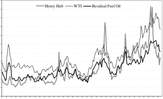
Figure 1: Real energy commodity prices (February 1990 – August 2006)

$-$1.00 $2.00 $3.00 $4.00 $5.00 $6.00 $7.00 $8.00 $9.00 $10.00 $11.00 F e b-90 A ug-90 F e b-91 A ug-91 F e b-92 A ug-92 F e b-93 A ug-93 F e b-94 A ug-94 F e b-95 A ug-95 F e b-96 A ug-96 F e b-97 A ug-97 F e b-98 A ug-98 F e b-99 A ug-99 F e b-00 A ug-00 F e b-01 A ug-01 F e b-02 A ug-02 F e b-03 A ug-03 F e b-04 A ug-04 F e b-05 A ug-05 F e b-06 A ug-06

Henry Hub WTI Residual Fuel Oil

2000$/mmbtu

Sources: Natural Gas Weekly and the Energy Information Administration

Figure 1 plots the real prices of three energy commodities expressed in real $2000/MMBtu (using an electricity price index as the deflator).2 It shows that natural gas prices have tended to fluctuate around residual fuel oil prices with alternating periods of several months to a year where they are persistently above or below the residual fuel oil

2

price. In some brief episodes, however, the natural gas price spikes substantially above the residual fuel oil price, and even the WTI price, in energy-equivalent terms.

In order to thoroughly investigate the relationship between the prices of natural gas, residual fuel oil, and WTI, and adjustments to deviations from that relationship, we develop and estimate an error correction model (ECM). In general, Engle and Granger (1987) have shown that if two series, and , are cointegrated, then there must exist an error correction representation of the dynamic system governing the joint behavior of

and over time. This system can be written as y_1t y_2t y_1t y_2t Δy_1t =α₁₀ +α₁₁Ω_t−1+ α_12,iΔy_1,t−i i=1 p₁

∑

∑

∑

∑

where is an error correction term representing the deviation from the equilibrium or cointegrating relationship between on . The coefficients on are speed of adjustment parameters measuring how fast and revert to their long run equilibrium relationship. Note that since and are cointegrated, the estimation of

on is superconsistent and the series Ω can be treated in the estimation of the ECM as if it were known. Each equation in the system above has the desirable property that if we are at long run equilibrium (Ω ) and there is no change in any of the other variables, there will be no change in and , provided the intercept terms ( and ) are equal to zero.

Ω_t−1 y_1,t−1 y_2,t−1 Ω_t−1 y_1t y_2t y_1t y_2t y_1t y_{2t t} t−1 =0 y_1t y_2t α₁₀ α₂₀

In this paper, we focus on the long run cointegrating relationships between the natural gas price, the residual fuel oil price, and the WTI price. We then extend the ECM representation to include some stationary exogenous variables, which allows us to identify some of the shocks that lead to departures from the long run equilibrium between prices. The estimated ECM also allows us to identify a causal ordering in price adjustment, and how fast that adjustment occurs.

II. Previous Research

Other authors have considered the cointegration of various energy prices. Of particular interest to us are papers that examine the cointegration of different commodities’ prices.3 One paper in particular considered the relationship between natural gas and residual fuel oil prices. Serletis and Herbert (1999) test for the existence of common trends in daily natural gas prices at the Henry Hub and Transco Zone 6, the price of power in PJM, and the price of residual fuel oil at New York Harbor from October 1996 through November 1997. They find that the three fuel prices are cointegrated and that Transco Zone 6 prices adjust significantly faster than do Henry Hub prices to deviations in their long run relationship. Serletis and Herbert also find that residual fuel oil prices show no significant adjustment to deviations in the long run relationship with either Henry Hub or Transco Zone 6 natural gas prices. However, the Transco Zone 6 natural gas price does appear to adjust to movements in the fuel oil price at New York Harbor. Their results thus support weak exogeneity of residual fuel oil prices in the system of equations. Similarly, the fact that the Transco Zone 6 price adjusts most quickly to both long run price relationships suggests that it is in a sense the “most endogenous” price of the three.

These findings are, to some extent, not very surprising. Transco Zone 6 is at the end of the Transco pipeline system, which delivers natural gas directly from the Gulf Coast to Middle Atlantic markets. Thus, cointegration of the two natural gas prices reflects the arbitrage possibilities inherent in the physical link. In addition, the Gulf Coast’s high connectivity to many regions implies that natural gas prices at the Henry Hub will be influenced by shocks in many local markets and thus not particularly responsive to the shocks in any one end-of-pipe market like Transco Zone 6. The finding that Transco Zone 6 natural gas prices also adjust to New York Harbor residual fuel oil prices indicates regional competition between those fuels.4 In addition, the weak exogeneity of the residual fuel oil price indicates that it may be responding to a different driver, such as crude oil.

3

There is also a literature examining the cointegration of a single commodity across different locations (see, for example, DeVany and Walls (1993, 1999) and Siliverstovs et al. (2005)).

4

Building on this analysis, Serletis and Rangel-Ruiz (2002) examine the existence of common price cycles in North American energy commodities using the daily prices of natural gas at the Henry Hub and WTI from 1991 through 2001. In addition, they studied cointegration of U.S. and Canadian natural gas prices. They concluded that natural gas prices at Henry Hub and AECO (a liquid pricing point in Alberta) demonstrate common cycles. While natural gas does not flow directly between the Henry Hub and AECO, it flows from both of those areas to common markets in the Middle Atlantic and the Midwest. Hence, these prices, like the Henry Hub and Transco Zone 6 prices, also appear to be linked via transportation differentials. Serletis and Rangel-Ruiz also found, however, that Henry Hub and WTI do not have common price cycles. They claim this decoupling of U.S. energy prices is a result of deregulation.

Villar and Joutz (2006) examine the apparent decoupling of the prices of WTI crude oil and Henry Hub natural gas in more detail, finding a cointegrating relationship between the two prices that exhibits a positive time trend. This indicates that the prices have a long run relationship that is slowly evolving rather than constant. Villar and Joutz estimate an error correction model that includes exogenous variables such as natural gas storage levels, seasonal dummy variables, and dummy variables for a few other transitory shocks. Their analysis supports the findings of Serlitis and Rangel-Ruiz (2002) that the price of WTI is weakly exogenous to the price of natural gas at the Henry Hub. Specifically, Villar and Joutz find that the price of natural gas adjusts to deviations in the long run evolving relationship, but these deviations do not affect the price of WTI. They also found that changes in natural gas prices tend to lag behind changes in crude oil prices.

Brown (2003) and Brown and Yücel (2006) observed that natural gas and crude oil prices had apparently decoupled on several occasions in the immediate past: once beginning in 2000 with natural gas prices becoming relatively high compared to crude oil prices, and again in 2005 with the relationship moving in the opposite direction. Brown argued in the 2003 paper that the futures markets supported the hypothesis that the movement away from the previous long run relationship in 2000 was likely to continue.

Brown and Yücel (2006) used an ECM to analyze weekly prices from January 1994 through July 2006. They found that the price series are cointegrated over this

period, indicating a stable long run relationship. However, they also found that a cointegrating relationship does not exist if they consider the shorter time period of June 1997 through July 2006. Proceeding with the estimated cointegrating relationship from the longer time series, they found that short run deviations from the estimated long run relationship could be explained by market fundamentals such as storage levels, weather (measured by the normal degree days for the week of the year and deviations from that norm), and the quantity of production shut-in due to hurricanes. They report that the price of natural gas at the Henry Hub responds significantly to the deviation from the long run relationship, changes in the prices of natural gas for the preceding two weeks, and the change in the price of oil one week earlier. Furthermore, they report that weather and storage levels both have significant effects on the price of natural gas by moving it temporarily away from the long run relationship to crude oil prices. Similar to previous studies, Brown and Yücel found the direction of causality is from the price of WTI to the price of Henry Hub, but not the other direction.

Bachmeir and Griffin (2006) also examine the evidence for cointegration within as well as across various commodity markets. Specifically, they find that various global crude oils are strongly cointegrated, but that the cointegrating relationship between the prices of different coals in the United States is not strong. Moreover, they report that cross-commodity cointegration in the United States is weak, and conclude that the market for energy can only be considered a single market for primary energy in the very long run. By contrast, Asche, Osmundsen and Sandsmark (2006), using data for the United Kingdom, report that the prices of crude oil, natural gas and electricity are cointegrated. Moreover, they find that there is a single market for primary energy in the United Kingdom in which price is determined exogenously by the global market for crude oil. In addition, they conclude that changes in regulatory structures and capacity constraints can make prices appear to be more or less cointegrated. Neither of these studies, however, considers the influence of exogenous variables, such as weather and inventories, on short run price adjustment. In addition, none of the studies we reviewed considered the influence of technology for the long run price relationships.

We also examine the relationship between oil and natural gas prices. Like Villar and Joutz, we use monthly data and attempt to find a stable cointegrating relationship

between natural gas and oil prices by adding an additional variable, but we consider technology rather than a time trend. More specifically, we assume that an electricity producer chooses among alternative fuels to minimize costs in dollars per MWh given as the fuel price multiplied by the heat rate. The substantial increase in combined-cycle power generating capacity over the past decade has lowered the capacity-weighted average heat rate for natural gas plants, effectively lowering the cost of producing electricity with natural gas relative to other fuels. Since a substantial amount of fuel competition occurs in the power sector, we would expect this technological change to have affected the long run relationship between natural gas and crude oil prices. Thus, we hypothesize that the increased efficiency of producing electricity with natural gas is responsible for the increasing price differential observed by Villar and Joutz.

We also follow both Villar and Joutz and Brown and Yücel by allowing market fundamentals such as storage levels and weather to influence the short run dynamic relationship between the prices. Finally, we follow the earlier papers by Serletis et al. in relating natural gas prices not to the price of crude oil but rather to the prices of the main competitive oil product, namely residual fuel oil. It is clear from Figure 1 that natural gas prices have tended to relate more closely to residual fuel oil than to crude prices. Nevertheless, we also allow crude prices to enter a system of equations that we estimate and thus to influence both of the other prices.

III. Data

As we noted in the previous section, much of the recent literature focuses on the relationship between the prices of crude oil and natural gas. Like Serletis and Herbert, we instead focus on the relationship between the prices of natural gas and residual fuel oil, although we also test for direct effects of crude oil prices on both end-user prices. Thus, we examine a system of three fuel prices: the price of natural gas at the Henry Hub (compiled from Natural Gas Weekly), the wholesale price of residual fuel oil and the price of WTI crude (the latter two series were obtained from the U.S. Energy Information Agency (EIA) web site). We examine the price of Henry Hub rather than natural gas prices in other regions because variations in basis differentials primarily reflect

transportation constraints, and hence the shadow value of scarce transportation capacity, rather than changes in the value of energy as such. Consistent with our theoretical framework, fuel prices are expressed in real $2000/MMBtu,5 and are deflated using industrial electricity retail prices, which most closely resemble a wholesale output price for the electricity sector.6

The heat rate data were constructed from two sources. The Environmental Protection Agency’s (EPA) NEEDS 2004 data provides the heat rates for many generating plants in the United States, but very few capacities and no information about month of first use. To obtain the additional information, the EPA data were matched to the facilities listed in the Energy Information Agency (EIA) Form-860 (Annual Electric Generator Report) in four steps.

• Step 1: Both the EIA and EPA datasets list plants by Facility ID and Generator number. For any plant where these matched exactly, the reported heat rate was matched to the EIA data.

• Step 2: If a plant did not have an exact match, but had the same Facility ID number, year of first use, prime mover, and fuel type, that plant from the EIA database was matched to the analogous plant in the EPA database.

• Step 3: For the remaining plants, a plant in the EIA database was assigned the average heat rate of facilities in the EPA database having the same year of first use, prime mover, and fuel type.

• Step 4: Finally, if a plant in the EIA database with a particular prime mover and fuel type had a year of first use that did not match the year of first use of any plants of that type in the EPA database, then it was assigned the average heat rate of plants in the EPA database with the same prime mover and fuel type and year

5

The conversion factors for energy content, obtained from the EIA web site, were 1.03 MMBtu per thousand cubic foot for natural gas, 6.287 MMBtu per barrel for residual fuel oil, and 5.800 MMBtu per barrel for WTI crude oil.

6

We related real, rather than nominal prices since general inflation could make any nominal price non-stationary and the general inflation rate would need to be included in the cointegrating relationship. This may obscure the real relationship between the different energy commodities. From the perspective of a cost-minimizing electricity producer, the relevant real input price for each fuel is the nominal price times the heat rate divided by the price of electricity. Taking logs, we then obtain the cointegrating relationship as estimated.

of first use closest to the actual year of first use, with a preference for using more modern plants where “closest” is ambiguous.7

The formula used for calculating the capacity-weighted heat rate for plants using fuel of type f in month t (HR_tf) is then given as

HR_tf =

(Capacity_i,tf *HeatRate_i,tf )

i

∑

Capacity_i,tf

i

∑

for all plants i using fuel f that were available for use at any time during month t. The EIA database provides as many as six energy sources for any one generator. Only the primary energy source was considered for the heat rate calculations. The use of the heat rate variable in our analysis restricts us to using data at the monthly frequency. One advantage of using monthly data, however, is that we can cover quite a long time series from February 1990 to October 2006.

Other variables included in the dynamic adjustment process include beginning of period inventory levels, variables reflecting weather conditions, and a variable to capture disruptions to Gulf of Mexico production as a result of hurricanes. The inventory

variables allow for short-term supply availability to either mitigate or exacerbate the effects of shocks on price movements. The weather variables are included to capture the effects that weather has on demand and hence price, and the hurricane variable is

included to capture the price impacts of short-term supply disruptions.

Inventory data was obtained from the EIA web site. For natural gas, we used working natural gas in storage at the end of the previous month (beginning of the current month), and, for residual fuel oil, we used monthly stocks at the end of the previous month measured in thousands of barrels.8

The weather variables were calculated using data on heating and cooling degree-days (HDD_tandCDD_t) from the National Oceanic and Atmospheric Administration

7

For example, suppose the year of first use for an EIA plant was 1999 and plants of that type appear in the EPA database with years of first use of 1998 and 2001, but not 1999. Then the average heat rate for the 1998 plants would be assigned. If plants in the EPA database had a year of first use of 1998 and 2000, but not 1999, the average heat rate for the 2000 plants would be assigned.

8

Natural gas inventories are measured in units of trillion cubic feet. We converted the residual fuel oil

(NOAA). To begin with, we calculated the 15-year average degree-days for each month ( and ) over the period 1990-2005. Since we also included monthly indicator variables in the dynamic adjustment equations, we did not include these normal seasonal variations in weather as explanatory variables.

HDDavg_t CDDavg_t

9

However, we did include deviations in heating and cooling degree-days in each month, measured as the actual values minus the 15-year average:

HDDdev_t =HDD_t −HDDavg_t CDDdev_t =CDD_t−CDDavg_t

We also included a measure of extreme winter weather events calculated as the top decile of the HDD distribution:10

HDDext_t = 0 if HDDdevt is not in the top 10% of values HDDdev_t if HDDdev_t is in the top 10% of values

⎧ ⎨ ⎪ ⎩⎪

We derived the hurricane variable by regressing federal offshore Gulf of Mexico natural gas production on a cubic time trend and a set of dummy variables representing periods when major hurricanes, as reported by NOAA, affected Gulf producing areas

NG_tGulf =α 0+α1t+α2t 2+α 3t 3+ δ jt_jDt_j t_j

∑

∑

In equation (1), j indexes the hurricanes that tracked through producing areas in the Gulf of Mexico within the sample period, indexes months for which hurricane j had a statistically significantly negative effect on production (relative to trend), and for

and 0 otherwise. The measure of production shut-in as a result of hurricanes is then taken to be t_j D_t j =1 t=t_j HurrShutIn_t = − δ_jt j D_t j t_j

∑

∑

An argument for including monthly effects rather than normal weather variables is that seasonal factors other than weather, such as the distribution of holidays or variations in the number of working days in a month, could influence demands for different types of energy commodities and hence prices.

10

A similar extreme cooling-degree day variable was neither numerically nor statistically significantly different from zero in any equation.

There are several motivations for our approach. First, a number of hurricanes over this period were believed to have had a lingering effect on production beyond the month in which they occurred. We sought a method that could detect the number of months affected and allowed the effects to moderate over time. Second, we wanted to allow for the possibility that different hurricanes affected production by different amounts. A simple dummy variable for the months of major hurricane strikes would treat all hurricanes identically. Third, the effects of hurricanes may be difficult to identify in the presence of changes in Gulf production for other reasons, such as depletion or new discoveries. We implicitly assume that these other influences are slow moving and thus can be approximated by a smooth polynomial time trend. The production shut-ins attributed to major hurricanes were then measured as statistically significant deviations from the smooth time trend coinciding with hurricane events in the Gulf producing areas. The method indicates that production was lost due to hurricanes during the following time periods: August-September 1992, October 1995, September 1998, September-October 2002, September-September-October 2004, and September-December 2005.11

We also included an indicator variable (Chicago) for February 1996. The first week of that month was very cold in many parts of the United States and produced extremely high demand. In particular, when coupled with low storage levels, the period witnessed unprecedented prices of natural gas in the Chicago market area, but those price increases were reversed quickly when the weather returned to normal in the following weeks. Although we have included variables to capture the effect of extreme weather on high prices, the 1996 incident had a peculiarly large effect on prices. This might be related to the then relatively new emergence of major market hubs and the offering of hub services such as “parks and loans,” which were not widely used at major hubs at that time.12 In any case, the February 1996 event is an outlier in analysis. The high prices in

11

We examined the effect of using simple dummy-variables in place of our measure of lost production. The coefficient on the hurricane shut-in variable became less significant but none of the remaining coefficients was materially affected.

12

The February 1996 episode is discussed in Natural Gas 1996: Issues and Trends which is available at

www.eia.doe.gov/oil_gas/natural_gas/analysis_publications/natural_gas_issues_and_trends/it96.html

The EIA notes on page 21 that “some industrial gas consumers paid more than $45.00 per MMBtu in Chicago in order to avoid pipeline imbalance penalties of over $60.00 per MMBtu.” On page 78 it claimed, “Other evidence that market centers are not being fully utilized is the size of the daily price spikes

experienced this past winter.” “Parks” (short-term gas storage) and “loans” (an advance of gas) can mitigate the impact of such combinations of severe weather and low storage levels because they allow

the Chicago area were transmitted back to Henry Hub due to the direct pipeline linkages between the Gulf Coast and the Chicago market area.

Finally, we allowed for seasonality in the adjustment process by including a set of monthly dummy variables. The natural gas price has a pronounced seasonal pattern, and although inventories rise and fall in an effort to partly mitigate seasonal price movements, they do not eliminate them completely. Inventory build is a function of current market conditions and expected future market conditions. If expectations are accurate, we might expect that controlling for inventory levels and normal weather conditions could explain seasonal movements in price. However, other factors such as the number of days in a month, and normal seasonal demand patterns in fuel consumption may not necessarily be captured by seasonal changes in inventories and heating or cooling degree days.13

IV. Analysis and Results

The premise of the ECM is that, although natural gas and residual fuel oil prices are each nonstationary (or more specifically integrated of order 1), there exists a stable long run relationship between them. Statistically, if two nonstationary variables are cointegrated, the residual after estimating their cointegrating relationship will be stationary. Phillips-Perron tests indicate that the levels of the logs of the three price variables and the relative heat rate variable are nonstationary and integrated of order one, I(1). The remaining variables are all stationary,I(0).14

consumers to meet contractual obligations and at the same time smooth the profile of capacity utilization on market area pipelines. Brownfield and greenfield expansions of pipeline infrastructure (i.e. – Northern Border and Alliance) occurred after the winter of 1996. These also increased access to Canadian supplies and storage and helped cope with similar problems in subsequent years.

13

We also investigated the use of actual weather rather than deviations from normal, but the monthly dummies remain significant. Thus, we adopt the approach taken here.

14

For ln(PP

NG

), the tests statistics are Z(ρ) = –8.725 and Z(τ) = –2.082 compared with Z(ρ) = –155.443 and

Z(τ) = –12.306 for ln(PNGP ). For ln(PP

rfo

), the tests statistics are Z(ρ) = –6.639 and Z(τ) = –1.666 compared

with Z(ρ) = –131.664 and Z(τ) = –10.836 for ln(PrfoP ). For ln(PP

WTI

), the tests statistics are Z(ρ) = –4.839

and Z(τ) = –1.345 compared with Z(ρ) = –143.120 and Z(τ) = –11.493 for ln(PWTIP ). For ln(HRrel), the

tests statistics are Z(ρ) = 1.363 and Z(τ) = 1.898 compared with Z(ρ) = –63.369 and Z(τ) = –6.133 for

ln(HRrel). The interpolated 10% critical value for Z(ρ) is –11.133, and for Z(τ) is – 2.573. The statistics

for the levels of the weather and storage variables are Z(ρ) = –161.882 and Z(τ) = –11.074 for HDDdev,

Z(ρ) = –136.925 and Z(τ) = –10.005 for CDDdev, Z(ρ) = –59.174 and Z(τ) = –5.426 for ngstor, and Z(ρ) =

To obtain a better understanding of the relationship among the prices and the relative heat rate variable, we estimated a vector auto-regression (VAR) on a vector Y of natural gas price, residual fuel oil price, WTI, and the relative heat rate using Johansen's maximum likelihood method.

t

15

Since the elements of are each I(1), the changes in the variables at time t, , are estimated as a function of and n lags of , where the optimal n is determined using the Akaike Information Criterion (AIC). The rank of the matrix multiplying is the number of cointegrating relationships in the system. The errors from the estimated cointegrating relationships are then used to construct an error correction model similar to that used in the Engle-Granger method.

Y_t

ΔY_t Y_t−1

ΔY_t

Y_t−1

The Johansen tests imply that there are two cointegrating relationships, and the AIC indicates that the optimal number of lags n is one. The two normalized cointegrating relationships are given as:16

ce₁ =lnP_tNG−0.3327−0.6540 (0.2612)lnPt rfo+ 3.5045 (1.7855)ln HR_tNG HR_trfo ⎛ ⎝ ⎜ ⎞ ⎠ ⎟ ce₂ =lnP_trfo+0.2053−0.8914 (0.0708)lnPt WTI .

Table 1 gives the corresponding estimated vector error correction model (VECM). The coefficients on the two cointegrating equations imply that only natural gas prices respond to divergences in the first long run relationship and only residual fuel oil prices adjust in response to deviations in . Furthermore, the negative coefficients imply that the subsequent adjustments will tend to restore the long run relationships.

ce₁ ce₂

15

For more information on maximum likelihood estimation in this context see Hamilton (1994).

16

The likelihood ratio test of the over identifying restrictions in this normalization yields a statistic

with a p-value of 0.378.

χ 1

2 ₌

Table 1: Estimated VECM model (without exogenous variables) Variable _ΔlnP t NG ΔlnP t rfo ΔlnP t WTI Δ lnHRrel_t ce_1,t−1 −_(0.04550.1699₎ *** 0.0010_(0.0259) −_(0.02630.0128₎ −_(0.00040.0004₎ ce_{2 ,t−1} 0.0031_(0.1002) −_(0.05700.1522₎ *** −_(0.05800.0092₎ −_(0.00080.0011₎ ΔlnP_t−NG₁ 0.1478_(0.0780)* 0.1465_(0.0444)*** 0.0536_(0.0451) −_(0.00070.0006₎ ΔlnP t−1 rfo 0.1306 (0.1835) −0.1718 (0.1044) * −0.2086 (0.1062) ** 0.0027 (0.0015) * ΔlnP t−1 WTI 0.1316 (0.1892) 0.4858(0.1077) *** 0.3275 (0.1096) *** −0.0015 (0.0016) ΔlnHRrel_t−1 −_(6.52750.0181₎ −_(3.71425.3305₎ −_(3.78013.6922₎ 0.6520_(0.0545)*** constant −_(0.01130.00001₎ −_(0.00640.00001₎ −_(0.00650.0002₎ −_(0.00010.0003₎*** R2 0.1249 0.2442 0.0625 0.5701 joint significance χ 7 2 ₌ 27.40 χ 7 2 ₌ 62.03 χ 7 2 ₌ 12.81 χ 7 2 ₌ 254.57

***- statistically significantly different from zero at the 1% level;**- statistically significantly different from zero at the 5% level;*- statistically significantly different from zero at the 10% level

The fact that neither changes in the WTI price nor changes in the relative heat rate variable respond to deviations in the two cointegrating relationships implies that both of these variables are weakly exogenous.17 The VECM also implies that the WTI price influences the remaining prices mainly through its effect on the residual fuel oil price. However, the estimated dynamic adjustment process in the VECM needs to be treated with some caution since the AIC test for lag length only considers uniform increments of all lags in all equations. In addition, the system may omit important exogenous variables

17

A joint test that the coefficients on ce1,t−1 and ce2 ,t−1 are zero except for ce1,t−1 in the natural gas price

adjustment equation and in the residual fuel oil price adjustment equation yields a test statistic

with a p-value of 0.4994. A test only that the coefficients on

2 ,t1

ce ₋

2 6 5.35

χ = ce_1,t−1 and are both zero in the

WTI equation yields a test statistic with a p-value of 0.8257, while a test that both coefficients on

and are zero in the relative heat rate equation yields a test statistic with a p-value of

0.0946. While this latter test is just significant at the 10% level, neither coefficient individually is

significantly different from zero (the corresponding z-statistics have p-values of 0.273 and 0.199). Finally,

a joint test that the coefficient on is zero in the residual fuel oil equation and the coefficient on

2 ,t1 ce ₋ 2 2 0.38 χ = 1,t1 ce ₋ ce_{2 ,t−1} χ₂2 =4.72 1,t1 ce ₋ ce_{2 ,t−1}

is zero in the natural gas equation yields a test statistic 2 with a p-value of 0.9986.

2 0.001 χ =

such as the weather and storage variables, and this could bias the estimated coefficients. To investigate more flexible dynamic adjustment models, we used the Engle-Granger two-step methodology.

Engle-Granger Methodology

The Engle-Granger method estimates each cointegrating relationship individually using ordinary least squares (OLS). Then, the errors from those cointegrating equations are included, along with the exogenous variables, in short run dynamic adjustment equations to explain adjustment to the long run equilibrium. Following the Johansen method results, we estimated equations (2) and (3) below by OLS:18.

lnP_tNG = 0.0701 (0.0913) +0.8779 (0.0849) lnP_trfo−3.0032 (0.5785) ln HRt NG HR_trfo ⎛ ⎝ ⎜ ⎞ ⎠ ⎟ +εt NG (2) (3) lnP_trfo = −0.2931 (0.0339) +0.9637 (0.0234) lnP_tWTI +ε_trfo

Since the Phillips-Perron test indicates both residuals are stationary, in each case there is a stable long run relationship and the parameter estimates will be superconsistent.19 The strong and statistically significant negative coefficient on the relative heat rate in (2) indicates that improvement in the heat rate of a natural gas-fired relative to an oil-fired generating plant has raised the price of natural gas relative to residual fuel oil as hypothesized. Furthermore, if we omit the relative heat rate from (2) the residual is closer to being nonstationary. In addition, if we use WTI rather than the residual fuel oil price in (2), the residual is nonstationary at the 1% level.

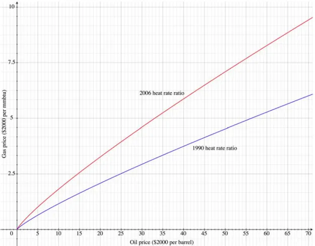
By substituting equation (4) into equation (2) we can express the relationship between WTI and natural gas as lnP_tNG = −0.1872+0.8460lnP_tWTI −3.0032ln HRt

NG HR_trfo ⎛ ⎝ ⎜ ⎞ ⎠ ⎟ . Solving this for a range of prices of WTI and relative heat rates can yield some insight into the behavior of the ratio of WTI to natural gas price. In particular, given the heat rate ratio in 1990, if the price of crude oil is $20 per barrel, the price of natural gas would be

18

The estimated standard errors are in parentheses below each estimated coefficient.

19

For , the test statistics are Z(ρ) = –30.793 (10% critical value –11.133) and Z(τ) = –4.033, which has

a MacKinnon approximate p-value of 0.0012. For , the test statistics are Z(ρ) = –25.686 and

Z(τ) = –3.719, which has a MacKinnon approximate p-value of 0.0039.

ε_tNG

ε t rfo

$2.08/MMBtu, yielding a 9.6-1 ratio. If the price of crude oil is $70, however, the price of natural gas would be $6.01/MMBtu, yielding a 11.6-1 ratio. Alternatively, if we change the heat rate ratio to reflect current conditions, a $20 per barrel and a $70 per barrel price of crude oil implies a price of natural gas of $3.27/MMBtu and $9.43, respectively, yielding a 6.1-1 and 7.4-1 ratios in each case. It is important to note that these are long run relationships.

Next, we estimate the short run dynamic adjustment to the long run relationships including stationary variables Xt, such as storage levels and weather, which affect short

run price adjustments. Using ˆεtNG to denote the predicted residual from (2), the ECM for

the change in natural gas prices can be written as

( )

( )

( )

( )

Equation (5) reveals that if we are at long run equilibrium, so that , and all other variables remain unchanged, then the price of natural gas will remain unchanged. Otherwise, if ( ), the price of natural gas is above (below) its long run equilibrium value, and if subsequent movements in the natural gas price will tend to restore the long run equilibrium relationship between fuel prices. The terms

and in (5) are polynomials in the lag operator while, since X is a vector, is a matrix of polynomials in the lag operator.

ˆ_tNG 0 ε = ˆ_tNG 0 ε > εˆ_tNG <0 β₀₁ <0 γ₀(L), δ₀(L) φ₀(L) α₀(L)

An equation similar to (5) can be written for the dynamic price adjustment of residual fuel oil as

( )

( )

( )

( )

rfo rfo NG rfo

t t t t WTI rfo t t P L X L P L P β β ε α γ δ φ ω − − Δ = + + + Δ + Δ + Δ + t L P (6)

where ˆε_trfo, the predicted residual from (3), represents deviations from the long run equilibrium between the residual fuel oil price and WTI. The interpretation of the variables in (5) is analogous to that for (4).

Figure 2: Implied long run relationship between the WTI and Henry Hub natural gas price (both in $2000) as a function of the WTI price per barrel

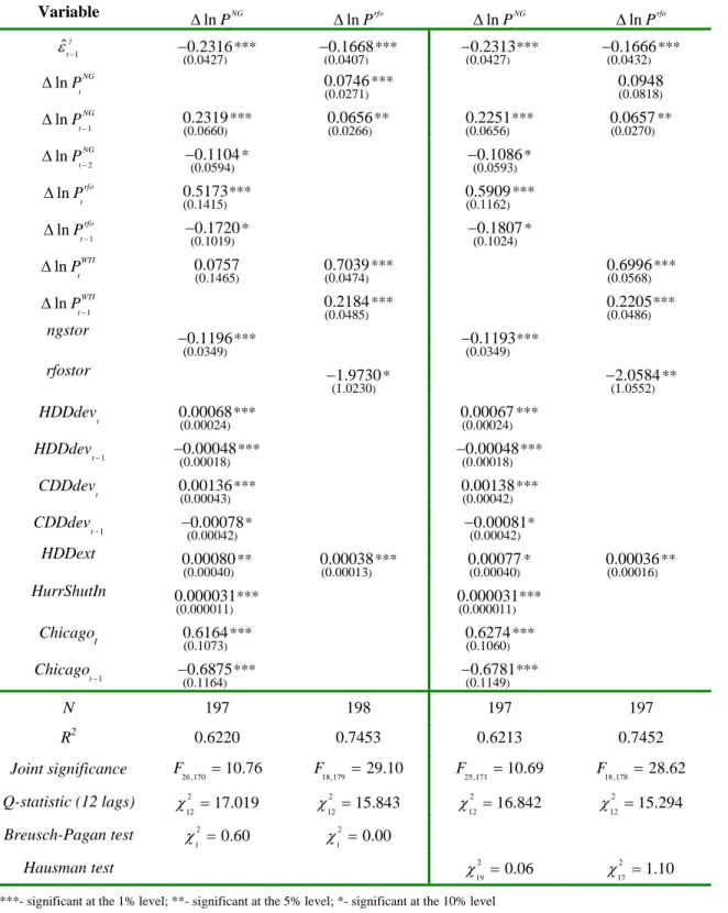
To provide a baseline for our subsequent analysis, we estimated (5) and (6) using OLS. Variables that proved individually and jointly insignificant at the 10% level, apart from the full set of monthly dummy variables and the change in WTI prices, have been eliminated from the equations. The results are reported in Table 2. The monthly dummy variables are not reported, but are available upon request.

Table 2: Error Correction Model Estimation Results OLS IV Variable _ΔlnP t NG _Δ lnP t rfo _Δ lnP t NG _Δ lnP t rfo 1 ˆj t ε₋ −0.2316 (0.0427) *** −0.1668 (0.0407) *** −0.2313 (0.0427) *** −0.1666 (0.0432) *** ΔlnP t NG _0.0746 (0.0271) *** 0.0948 (0.0818) ΔlnP t−1 NG 0.2319 (0.0660) *** 0.0656 (0.0266) ** 0.2251 (0.0656) *** 0.0657 (0.0270) ** ΔlnP t−2 NG −_0.1104 (0.0594) * −0.1086 (0.0593) * ΔlnP t rfo 0.5173 (0.1415) *** 0.5909 (0.1162) *** ΔlnP t−1 rfo − 0.1720 (0.1019) * −0.1807 (0.1024) * ΔlnP t WTI 0.0757 (0.1465) 0.7039 (0.0474) *** 0.6996 (0.0568) *** ΔlnP t−1 WTI _0.2184 (0.0485) *** 0.2205 (0.0486) *** ngstor _−0.1196 (0.0349) *** −0.1193 (0.0349) *** rfostor _−1.9730 (1.0230) * −2.0584 (1.0552) ** HDDdev t 0.00068_(0.00024)*** 0.00067_(0.00024)*** HDDdev_t−1 −0.00048 (0.00018) *** −0.00048 (0.00018) *** CDDdev t 0.00136_(0.00043)*** 0.00138_(0.00042)*** CDDdev t−1 −_(0.000420.00078₎ * −_(0.000420.00081₎ * HDDext _0.00080 (0.00040) ** 0.00038 (0.00013) *** 0.00077 (0.00040) * 0.00036 (0.00016) ** HurrShutIn _0.000031 (0.000011) *** 0.000031 (0.000011) *** Chicago_t 0.6164 (0.1073) *** 0.6274 (0.1060) *** Chicago_t−1 −0.6875 (0.1164) *** −0.6781 (0.1149) *** N 197 198 197 197 R2 0.6220 0.7453 0.6213 0.7452 Joint significance F 26 ,170 =10.76 F18,179 =29.10 F25,171 =10.69 F18,178 = 28.62 Q-statistic (12 lags) χ 12 2 ₌ 17.019 χ 12 2 ₌ 15.843 χ 12 2 ₌ 16.842 χ 12 2 ₌ 15.294 Breusch-Pagan test χ 1 2 ₌ 0.60 χ 1 2₌ 0.00 Hausman test χ 19 2 ₌ 0.06 χ 17 2 ₌ 1.10

Several features of these estimated equations are of interest. First, all variables have the expected signs, and diagnostic tests indicate the models fit the data reasonably well while leaving uncorrelated and homoskedastic residuals. Second, the change in the residual fuel oil price has a much larger effect in the natural gas price equation than vice versa. Third, while the contemporaneous (and lagged) change in WTI has a large effect in the residual fuel oil equation, its coefficient in the natural gas equation is much smaller and not statistically very different from zero. This suggests that crude oil prices influence natural gas prices mainly via competition with residual fuel oil as hypothesized. A potential problem with the OLS estimates, however, is that the prices of residual fuel oil and natural gas may be jointly determined. To examine this possibility, we re-estimated the equations using instrumental variables (IV).

In order to estimate (4) and (5) using IV we need a suitable set of instruments. Such variables should be exogenous or predetermined variables that are directly correlated with one of the price changes but not with the other so that they would influence the dependent variable only via their effect on the included endogenous variable. As instruments in each equation, we used the weather variables, own inventories, lagged values of own price, and current and lagged values of WTI. The weather variables are exogenous, and on the basis of the OLS results, it would appear that only the most extreme weather in winter directly affects the change in residual fuel oil prices (holding other variables in (5) fixed). We therefore used the contemporaneous and lagged heating and cooling degree-day deviations, as well as the hurricane shut-in variable, as instruments for the change in natural gas prices in (5).

We also used beginning-of-month inventories as an instrumental variable in each equation. Beginning-of-month inventories should signal the availability of supply entering that month, and thus influence the change in price over the rest of the month. However, inventories at the beginning of the month should not be influenced by the change in price that subsequently occurs over the following month.

The OLS results also indicate that the change in natural gas prices from two months ago (that is, the twice-lagged change) does not directly affect the contemporaneous change in residual fuel oil price, but does affect the contemporaneous change in the natural gas price. Hence, the twice-lagged change in natural gas price is

also a reasonable instrument for the contemporaneous change in natural gas price in the residual fuel oil price equation. Similarly, the OLS results imply that the twice-lagged change in residual fuel oil prices does not directly affect the contemporaneous change in the natural gas price. Hence, we also use it as an instrument for the contemporaneous change in residual fuel oil prices in the natural gas price equation.

Since the price of WTI is determined in the world oil markets, it is effectively exogenous with respect to changes in the U.S. markets for residual fuel oil and natural gas. The OLS results also suggest that although changes in the residual fuel oil price are highly dependent on changes in WTI, the influence of WTI on natural gas prices is not statistically significant once the effects of residual fuel oil prices have been taken into account. We therefore also used the contemporaneous and lagged change in the WTI price as instruments for the change in the residual fuel oil price in (4) (after dropping the change in WTI price as an exogenous regressor in that equation).

Table 2 also presents the resulting IV estimates of equations (5) and (6). Hausman tests for exogeneity suggest that one can treat the change in residual fuel oil price as exogenous in the natural gas price adjustment equation and vice versa. The estimated OLS and IV coefficients are generally very similar. However, the coefficient on changes in natural gas prices in (5) becomes statistically insignificant, while the estimated effect of residual fuel oil prices in (4) increases in both magnitude and statistical significance. This suggests that the residual fuel oil price causes movements in the natural gas price, but that the converse is not true. In turn, while the price of WTI influences the price of natural gas at the Henry Hub, it does so indirectly through its effect on the price of residual fuel oil.

We conclude that the natural gas price adjustment equation can be estimated using OLS in spite of the inclusion of the contemporaneous movement in the residual fuel oil price. It will differ from the OLS equation in Table 2, however, since the WTI price term will also be excluded. Similarly, the residual fuel oil price adjustment equation can also be estimated using OLS, but will differ from the OLS equation in Table 2 since the contemporaneous change in the natural gas price will be excluded. The resulting final regression equations are presented in Table 3.

Table 3: Final OLS and VECM Results OLS VECM Variable ΔlnP t NG ΔlnP t rfo ΔlnP t NG ΔlnP t rfo ΔlnP t WTI 1 ˆj t ε₋ −0.2305 (0.0426) *** −0.1800 (0.0411) *** −0.2306 (0.0407) *** −0.1926 (0.0396) *** ΔlnP t−1 NG _0.2269 (0.0652) *** 0.0692 (0.0271) ** 0.2259 (0.0645) *** 0.0738 (0.0263) *** ΔlnP t−2 NG −_0.1095 (0.0592) * −0.1092 (0.0562) ** ΔlnP t rfo _0.55729 (0.0916) *** 0.6060 (0.2290) *** −0.0528 (0.0865) ΔlnP t−1 rfo −_0.1768 (0.1012) * −0.1869 (0.1051) * ΔlnP t WTI _0.7335 (0.0470) *** 0.1726 (0.1844) ΔlnP t−1 WTI _0.2193 (0.0493) *** 0.3160 (0.0591) *** 0.2158 (0.0977) ** ngstor −0.1184 (0.0348) *** −0.1198 (0.0339) *** rfostor −2.1658 (1.0391) ** −2.5987 (1.0088) ** HDDdev t 0.00067 (0.00024) *** 0.00069 (0.00022) *** HDDdev t−1 −0.00048 (0.00018) *** −0.00048 (0.00017) *** CDDdev_t 0.00138_(0.00042)*** 0.00139_(0.00040)*** CDDdev t−1 −0.00081 (0.00042) * −0.00079 (0.00039) ** HDDext 0.00078 (0.00040) * 0.00047 (0.00013) *** 0.00075 (0.00038) * 0.00045 (0.00012) *** HurrShutIn 0.000031_(0.000011)*** 0.000031_(0.000010)*** Chicago_t 0.6253 (0.1056) *** 0.6180 (0.1013) *** Chicago t−1 −0.6786 (0.1149) *** −0.6901 (0.1070) *** N 197 198 197 197 197 R2 0.6220 0.7346 Joint significance F 25,171 =11.23 F17 ,180 =29.30 Q-stat (12 lags) χ 12 2 ₌ 17.087 χ 12 2 ₌ 17.287 χ 108 2 ₌ 132.133 * Heteroskedasticity or ARCH χ1 2 ₌ 0.78 χ 1 2 ₌ 0.32 χ 12 2 ₌ 12.018 χ 12 2 ₌ 8.388 χ₁₂2 =14.525

The right panel of Table 3 includes a vector error correction estimate of the same model using the OLS estimates of the cointegrating equations. These estimates were obtained by three stage least squares using the program JMulti (Lütkepohl and M. Krätzig, 2004). The two sets of estimates in Table 3 are similar except for the coefficients on the current change in the WTI price in the residual fuel oil equation. A potential problem with estimating a system of equations is that if one of the equations is misspecified, the estimates in the other equations can be affected. Since developing a model of the world oil market is beyond the scope of our analysis, the model for the change in the WTI real price is rudimentary. It includes only the variables found to be statistically significantly different from zero in Table 1. Even then, the lagged change in the residual fuel oil price is not statistically significant in the VECM formulation.

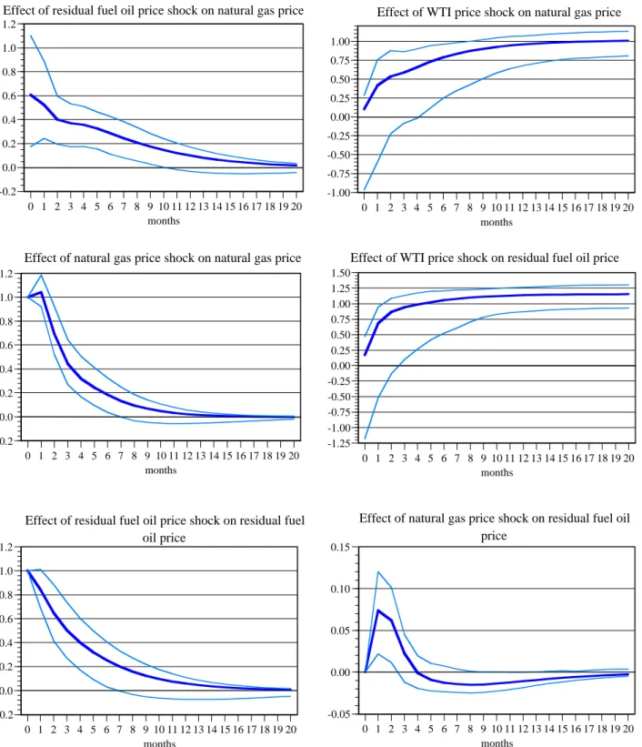
Despite the potential problems, we needed the VECM formulation to calculate the impulse response functions for the model. These are graphed in Figure 3, along with 95% Hall bootstrap confidence intervals obtained with 250 bootstrap replications. It can be seen from the impulse response functions graphed in figure 3 that both the residual fuel oil price and the natural gas price adjust proportionately in the long run to movements in the WTI price, with the residual fuel oil price approaching full adjustment within a few months, and the natural gas price taking a few months longer. In the cases where shocks occur to variables other than WTI, they have a period of significantly positive effect on the residual fuel oil and natural gas prices, but the effects ultimately disappear over time. Since only lagged natural gas price has an effect on the residual fuel oil price, the impulse response for residual fuel oil on a natural gas price shock is non-monotonic, or it increases then decreases.

The price adjustments are stable in the long run because the estimated coefficients on deviations from the long run relationships, ˆNG₁

t

ε₋ andˆrfo₁

t

ε₋ , are negative, as seen in Table 3. Thus, deviations from the long run relationships cause both natural gas and residual fuel oil prices to return to their long run equilibrium relationships with residual fuel oil and WTI, respectively.

Figure 3: Impulse response functions (VECM with exogenous variables) 0 1 2 3 4 5 6 7 8 9 10 11 12 13 14 15 16 17 18 19 20 -0.2 0.0 0.2 0.4 0.6 0.8 1.0 1.2 months

Effect of natural gas price shock on natural gas price

0 1 2 3 4 5 6 7 8 9 10 11 12 13 14 15 16 17 18 19 20 -0.2 0.0 0.2 0.4 0.6 0.8 1.0 1.2 months

Effect of residual fuel oil price shock on natural gas price

0 1 2 3 4 5 6 7 8 9 10 11 12 13 14 15 16 17 18 19 20 -1.25 -1.00 -0.75 -0.50 -0.25 0.00 0.25 0.50 0.75 1.00 1.25 1.50 months

Effect of WTI price shock on residual fuel oil price

0 1 2 3 4 5 6 7 8 9 10 11 12 13 14 15 16 17 18 19 20 -0.05 0.00 0.05 0.10 0.15 months

Effect of natural gas price shock on residual fuel oil price 0 1 2 3 4 5 6 7 8 9 10 11 12 13 14 15 16 17 18 19 20 -1.00 -0.75 -0.50 -0.25 0.00 0.25 0.50 0.75 1.00 months

Effect of WTI price shock on natural gas price

0 1 2 3 4 5 6 7 8 9 10 11 12 13 14 15 16 17 18 19 20 -0.2 0.0 0.2 0.4 0.6 0.8 1.0 1.2 months

Effect of residual fuel oil price shock on residual fuel oil price

The estimated coefficients shown in Table 3 also indicate that weather plays a very important role in short run price movements. Deviations from normal weather, HDDdev and CDDdev, tend to only influence the natural gas price, but the extreme deviations in cold weather, HDDext, do have a significant impact on residual fuel oil prices. With regard to natural gas price adjustment, the almost complete reversal of the coefficients on HDDdev and CDDdev after one period suggests that the effects of unusual weather on natural gas prices are short-lived. In addition, extremely cold weather in Chicago in February 1996 had an especially large effect on natural gas prices, but the change was reversed the following month.20

The estimated negative coefficients on the product inventory variables imply that higher beginning-of-month storage leads to lower prices over the month, holding all else equal. This follows from the fact that inventories represent readily available supply in any given month, and ample supply will tend to reduce prices. As might be expected, hurricanes tend to have a significant impact on natural gas prices as supply is reduced. The estimated coefficient implies that for every billion cubic feet of production that is shut-in as a result of a hurricane in the Gulf of Mexico, natural gas prices at the Henry Hub increase by approximately $1.03/MMBtu (=exp 0.000032 *1000

(

)

Finally, the monthly dummies (not reported in Table 2) reveal some seasonal tendency in the price series that is not captured by the other variables. To begin, as estimated, the variables must be interpreted as relative to January. With regard to natural gas, holding all other variables constant, from August through December prices increase more than they do in January, but from February through July they increase less than they do in January. Thus, in general, we find evidence that natural gas prices begin to rise in the late summer through the winter, but decline from winter through the late summer.

20

There is considerable evidence that the Chicago incident is an outlier. If and are

omitted from the regressors, the standard deviation of the residuals rises to 0.1090 from 0.0919, the minimum residual falls to -0.4930 from -0.2528, and the maximum rises from 0.2290 to 0.5370. A test for

adding back to the regressors yields a t-statistic of 5.35, while the test for adding back

yields a t-statistic of -5.34. In addition, the overall regression fit is adversely affected when these variables

are omitted. The R

t

Chicago Chicago_t−1

t

Chicago Chicago_t−1

2

of the regression falls to 0.4682 from 0.6214, while the test for joint significance of the

included variables becomes instead of . Furthermore, omitting these variables

substantially reduces the magnitude and statistical significance of the coefficients of

, while raising the magnitude (and standard error) of the coefficient of .

23 ,173 6.62 F = F_{25 ,171} =11.23 1 1 ln NG, ln rfo and t t P₋ P₋ HDDext Δ Δ ngstor