On cumulative frequency/probability distributions and confidence intervals.
R.J. Oosterbaan
A summary of www.waterlog.info/pdf/binomial.pdf
Frequency analysis is the analysis of how often, or how frequent, the value of an observed phenomenon occurs in a certain range with an upper and lower limit. It applies to a record of length N of observed data X1, X2, X3, . . .XN on a variable phenomenon X.
The record may be time-dependent (e.g. rainfall measured in one spot) or space-dependent (e.g. crop yields in an area) or otherwise.
The cumulative frequency MXr of a reference value Xr is the number of observed values X in
the range less than or equal to Xr.
The relative cumulative frequency Fc can be calculated from: Fc = MXr / N, where N is the
number of data. Briefly this expression can be noted as: Fc = M / N
A cumulative probability distribution (CPD) is a distribution of the probability Pc that an event (X) is smaller than (or at most equal to) a reference value Xr. This probability is called cumulative probability.
The CPD can be estimated from the observed cumulative frequency distribution (CFD), which is then considered as a sample from the CPD. The cumulative probability is then defined as Pc = Fc.
When M = N, i.e. X = Xmax (the maximum value in the range), one finds Fc = 1. To create the possibility that there may be X values larger than Xmax, the value of Fc can be redefined as Fc = M / (N +1).
When the observed data of X are arranged in ascending order , the minimum first and the maximum last, and Ri is the rank number of the observation Xi, where the affix i indicates the serial number in the range of ascending data, then the cumulative frequency is Fc = Ri / (N+1) and the estimated cumulative probability will be Pc = Ri / (N+1).
In literature, there are mathematical expressions of many different probability distributions and CPD’s. One can try to fit a CPD to an observed CFD, optimizing the parameters of the CPD so that the sum of the squares of the differences Pc and Fc is minimum. The fitted CPD is then an estimate of the true CPD from which the CFD is considered a sample.
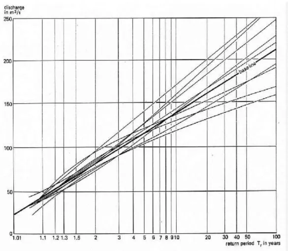
In theory, a sample is subject to a sampling error. When taking different samples, one may find different fitted CFD’s (figure 1, next page). Therefore the estimated CPD may deviate from the true CPD from which the CFD is a sample. To estimate the possible error, a confidence analysis can be made.
Figure 1. Copy of figure 6.2 in http://www.waterlog.info/pdf/freqtxt.pdf illustrating different outcomes of samples from the same probability distribution
An observed value X can either be greater than a reference value Xr (X > Xr) not greater than Xr ( X ≤ Xr). The well known binomial probability distribution (BPD) deals with phenomena that either occur or do not occur. It gives the probability that an event actually occurs M times in a sample of size N when the probability of occurrence is Po. Therefore, BPD can be used to estimate confidence intervals for the CPD estimated from a CFD.
An example: assuming the value Xr has a true cumulative probability Pct, then one can estimate with the BPD what the probability is that , in a sample of size N , the number of occurrences is M+1, M+2 . . . N and M, M-1, M-2, . . . 0. Also, one can find the probability of the number of occurrences greater than a relatively large number Mg (>M) and less than a relatively small number Ms (≤ M ). Calling these probabilities Pmg and Pms respectively, one can obtain the confidence interval Pmg – Pms for Mg and Ms.
For example, assuming Pmg = 95% and Pms = 5%, while the corresponding M values are Mgc and Msc, one finds a 90% confidence interval as Mgc – Msc. Converting these value into relative frequencies Fgc = Mgc/(N+1) and Fsc = Msc/(N+1), one obtains the confidence
interval in terms of cumulative of frequencies as Fgc – Fsc, which can serve as an estimate for the confidence interval in terms of Pc as Pcg – Pcs, where Pcg is the upper and Pcs the lower confidence limit.
The disadvantage of the BPD is its discontinuity (figure 2, next page), and the values of Mg and Ms are whole numbers (integers), so that the value of Pmg and Pms for real values with a decimal part of must be estimated by interpolation (figure 3). This problem may be solved as follows.
The standard deviation of the binomial distribution as a fraction of N (the relative standard deviation) equals
SDb = √ Pc(1-Pc)/N (eqn. 1)
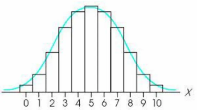
When Pc = 0.5, the BPD is symmetrical and coincides with the corresponding normal distribution with mean N.Pc and a standard deviation equal to SDb (figure 4). Hence, here the confidence limits can be approximated by the same method used for the normal distribution as
Pcg = Pc + t.SDb (eqn. 2)
and
Pcs = Pc – t.SDb (eqn. 3)
where t is the value of the variable in Student’s distribution corresponding to the level of certainty one wishes to achieve. For example, when N > 10, the t-value for 90% certainty is close to 1.7
A calculator for the t-distribution can be downloaded from http://www.waterlog.info/t-tester.htm and a calculator for the normal distribution from
http://www.waterlog.info/normdis.htm With these one can verify that for larger values of N (>10) the t-values and the x-values of the normal distribution at the same certainty level do not differ much relatively.
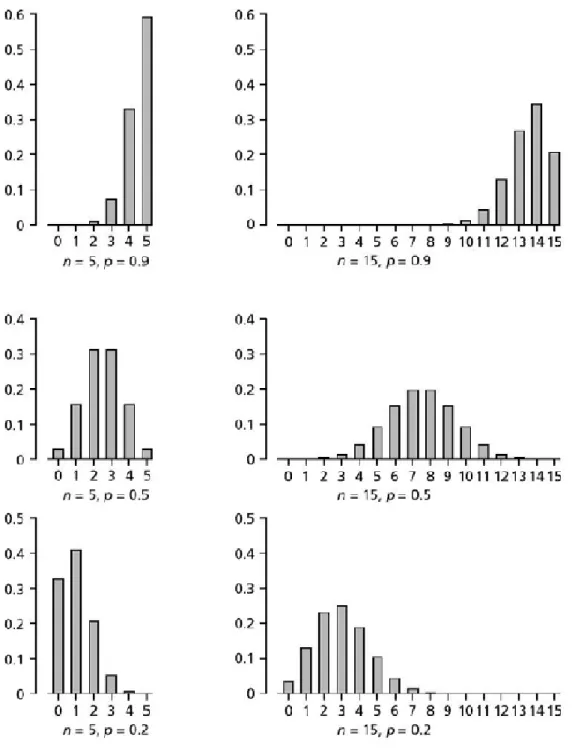
At Pc values other than 0.5, the binomial distribution becomes skew (figure 2). A simple method to take the skewness into account for the determination of the confidence limits is by making use of the Pc values themselves as a weight factor as follows:
Upper confidence limit: Pcg = Pc + 2(1-Pc).t.SDb = Pc + 3.4(1-Pc)SDb (eqn. 4) Lower confidence limit: Pcs = Pc – 2Pc.t.SDb = Pc - 3.4 Pc.SDb (eqn. 5) For higher values of Pc (e.g. Pc = 0.9) the addition to Pc to obtain the Pcg becomes small while the subtraction from Pc to obtain the Pcs is getting larger. For lower values of Pc, the reverse is true. For Pc = 0.5, both equations give the same result and they equal the
expressions (eqn. 2 and eqn. 3) given before. Since the maximum value of Pc is unity, the value of Pcg can never become greater than unity, as required, and since the minimum value of Pc equals zero the value of Pcs can never be less than zero, as required.
Figure 2. The binomial distribution is symmetrical when Pc (p in the figure) is 0.5 as can be seen in the middle two graphs. It is skew to the left at higher p values (top two graphs) and skew to the right at lower p values (bottom two figures)
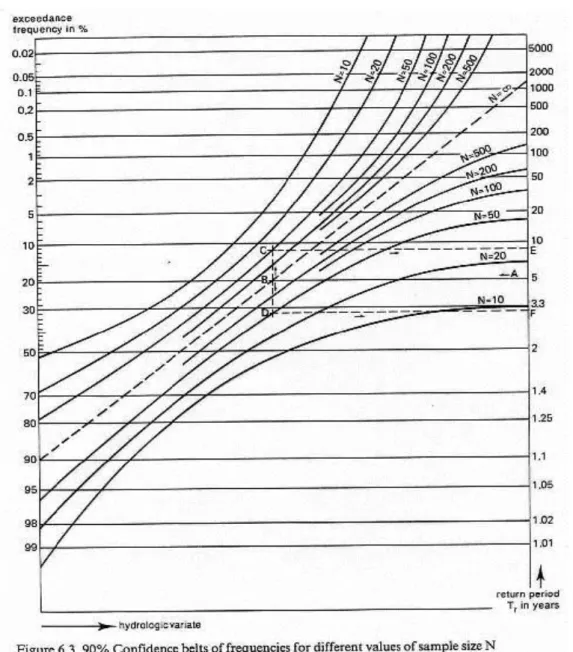
Figure 3. Copy of Figure 6.3 in http://www.waterlog.info/pdf/freqtxt.pdf illustrating a graphical procedure to arrive at 90% binomial confidence intervals.
Example of the use of figure 3. It is based on return periods (Tr), but it can also be used for exceedance frequency (Fe = 1 – cumulative frequency). Tr = 1/Fe.
- Enter the graph on the vertical axis with a return period of Tr = 5, (point A), and move horizontally to
intersect the baseline, with N = ∞, at point B;
- Move vertically from the intersection point (B) and intersect the curves for N = 50 to obtain points C and D; - Move back horizontally from points C and D to the axis with the return periods and read points E and F; - The interval from E to F is the 90% confidence interval of A, hence it can be predicted with 90% confidence
that Tr is between 3.2 and 9 years. Nomographs for confidence intervals other than 90% can be found in
literature (e.g. in Oosterbaan 1988).
Oosterbaan, R.J. 1988. Frequency predictions and their binomial confidence limits. In: Economic Aspects of flood control and non-structural measures, Proceedings of the Special Technical Session of the International Commission on Irrigation and Drainage (ICID), Dubrovnik, pp. 149-160.
Figure 4. The symmetrical but discontinuous (stepwise) binomial distribution and the corresponding continuous (smooth) normal distribution with the same mean and standard deviation (blue curve).
Confidence in interval of the return period.
The return period T is defined as
Tr = 1/(1-Pc) (eqn. 6)
Mathematically the upper (Ut) and lower (Lt) confidence limits of the return period T could be expressed as
Ut = 1 / (1 – Pcg) (eqn. 7)
Lt = 1 / (1 – Pcs) (eqn. 8)
where Pcg and Pcs are as defined in eqn. 4 and 5.
However, this leads to Ut values closer to the calculated/expected Tr values than Lt. One would expect a much higher Ut value, because the probability distribution of the return period should be skew to the right. Therefore, arbitrarily, the following adjustment can be made:
D = Ut – Lt (giving the entire confidence range) (eqn. 9)
Ut = Tr + 0.67 D (eqn. 10)
Lt = Tr – 0.33D (eqn. 11)
Confidence interval of the X value at a certain cumulative probability.
The cumulative probability (Pc) can be written as a function f of X:
Hence, X can be written as the inverse function f
’
of Pc:X = f
’
(Pc) (eqn. 13)With this inverse function, the upper confidence limit Ux and the lower limit Lx of X at Pc can be calculated as:
Ux = f
’
(Pcg) (eqn. 14)Lx = f