INSTITUT FÜR INFORMATIK

(1)

INSTITUT F ¨

UR INFORMATIK

Monocular Pose Estimation Based on

Global and Local Features

Marco Antonio Chavarria Fabila

Bericht Nr. 0922

November 2009

CHRISTIAN-ALBRECHTS-UNIVERSIT ¨

AT

(2)

(3)

Institut f ¨ur Informatik der

Christian-Albrechts-Universit¨at zu Kiel Olshausenstr. 40

D – 24098 Kiel

Monocular Pose Estimation Based on Global and

Local Features

Marco Antonio Chavarria Fabila

Bericht Nr. 0922 November 2009

e-mail: mc@ks.informatik.uni-kiel.de

Dieser Bericht gibt den Inhalt der Dissertation wieder, die der Verfasser im Januar 2007 bei der Technischen Fakult¨at der

Christian-Albrechts-Universit¨at zu Kiel eingereicht hat. Datum der Disputation: 05. Juni 2009.

(4)

(Kiel)

2. Gutachter

Prof. Bodo Rosenhahn

(Hannover)

(5)

ABSTRACT

The presented thesis work deals with several mathematical and practical aspects of the monocular pose estimation problem. Pose estimation means to estimate the po-sition and orientation of a model object with respect to a camera used as a sensor el-ement. Three main aspects of the pose estimation problem are considered. These are the model representations, correspondence search and pose computation. Free-form contours and surfaces are considered for the approaches presented in this work. The pose estimation problem and the global representation of free-form contours and surfaces are defined in the mathematical framework of the conformal geomet-ric algebra (CGA), which allows a compact and linear modeling of the monocular pose estimation scenario. Additionally, a new local representation of these entities is presented which is also defined in CGA. Furthermore, it allows the extraction of local feature information of these models in 3D space and in the image plane. This local information is combined with the global contour information obtained from the global representations in order to improve the pose estimation algorithms. The main contribution of this work is the introduction of new variants of the iterative closest point (ICP) algorithm based on the combination of local and global features. Sets of compatible model and image features are obtained from the proposed local model representation of free-form contours. This allows to translate the correspon-dence search problem onto the image plane and to use the feature information to develop new correspondence search criteria. The structural ICP algorithm is de-fined as a variant of the classical ICP algorithm with additional model and image structural constraints. Initially, this new variant is applied to planar 3D free-form contours. Then, the feature extraction process is adapted to the case of free-form surfaces. This allows to define the correlation ICP algorithm for free-form surfaces. In this case, the minimal Euclidean distance criterion is replaced by a feature corre-lation measure. The addition of structural information in the search process results in better conditioned correspondences and therefore in a better computed pose. Fur-thermore, global information (position and orientation) is used in combination with the correlation ICP to simplify and improve the pre-alignment approaches for the monocular pose estimation. Finally, all the presented approaches are combined to handle the pose estimation of surfaces when partial occlusions are present in the image. Experiments made on synthetic and real data are presented to demonstrate the robustness and behavior of the new ICP variants in comparison with standard approaches.

(6)

(7)

ACKNOWLEDGMENT

I thank to all the people who in a way or another helped me in the elaboration of this thesis work. First at all, I thank to my supervisor Prof. Dr. Gerald Sommer for giving me the opportunity to collaborate in the Cognitive System Group. I thank him for supporting me to obtain my scholarship, for suggesting me this interesting research topic, for his advice and comments to solve the different research problems and for supporting the conferences I visited. Especially, I want to thank him for his patience also in the difficult moments.

Furthermore, I thank all the members and ex-members of the Cognitive System Group for their help and support. Especially to Bodo Rosenhahn and Oliver Granert with whom I had the first discussions about geometric algebras and the pose estima-tion problem. That helped me a lot to understand the main theoretical and practical aspects of the pose estimation problem. I thank the help and support of Nils Siebel, Christian Perwass, Yohannes Kassahun, Di Zang, Florian Hoppe, Herward Prehn and Christian Gebken who always were ready to answer my questions and to share valuable comments, which in some way or another are reflected in this work. The friendly and pleasant atmosphere in the group made the research work very stimu-lating. I also thank to my colleagues Sven Buchholz, Lennart Wietzke and Stephan Zeitschel for proofreading the different chapters of this thesis work and for sug-gesting me improvements of the contents and redaction. I appreciate the help of the technical staff, Henrik Schmidt, Gerd Diesner and the secretaries of the group Franc¸oise Maillard and Armgard Wichmann. A special thank to the staff of the In-ternational Center of the Christian Albrechts University for their help during my stay at the University of Kiel.

I thank the Mexican Council of Science and Technology (CONACYT) for giving me the scholarship (number of registry: 144161) to support of my doctoral studies. In a similar way, I thank the German Service of Academic Exchange (DAAD) for giving me the opportunity me to participate in a language course, where I started to learn more about the culture of the German people.

Last, but not at least, I thank my family for their unconditional support and encouragement. Thanks to my parents Martin and Gloria, to my sister Diana and to my brother Efrain. I dedicate this thesis work to my family and especially to my beloved wife Caterina Maria Carrara, whose encouraging and loving words during these years gave me the strength to accomplish this work.

(8)

(9)

Chapter 1 INTRODUCTION

Computer vision and robotic systems are among the most innovative and impor-tant research topics with an enormous potential of practical applications. No other technical innovation has developed so fast than computers in the recent years. Since the first personal computer developed in the seventy years, every new generation of computers is faster, cheaper and more compact. Hence, efficient applications based on computer systems are available nowadays for almost every institution, industry and individuals in almost all aspects of modern life. This has also allowed the use of robots in a wide variety of applications, e.g. in entertainment systems, industrial applications and missions to explore other planets among others. Robots are used in those situations where the work is too dangerous, hard and repetitive and in cases where humans can not perform a certain task with high accuracy. In this context, a big challenge for research has been to emulate in robots the basic human behav-ior to solve problems. That means, the way that humans perceive information and take decisions to solve a specific problem. In this framework, the perception-action cycle defines the way that robots interact with their environment to solve a certain task. Once that all possible informations of the environment have been acquired and interpreted in the perception phase, a set of decisions are taken in the action phase.

Let us concentrate on the perception phase. A description about the size and structure of the robot’s environment must be generated. On the other hand, the location of the robot and any other objects must be determined in order to plan a possible action strategy. In order to obtain this information, modern robot systems are equipped with a large variety of sensor elements. The most adequate sensors are chosen depending on the specific task to be solved. Infrared or ultrasonic sen-sors are commonly used for robot navigation applications. Thermal and humidity sensors are also used to work in industrial environments. Modern sensors based on GPS (global positioning systems) are used for robot localization and navigation. Although these systems are able to deliver very precise measurements, they are lim-ited to a specific parameter of the world.

In contrast to the above mentioned sensor elements, the use of visual information has become more popular in the last years. The most important way to get infor-mation about the world is through vision. Vision allows humans to perceive a huge amount of information, e.g. shape, color, dimension, etc. It is the principle to

(14)

con-struct more general and abstract interpretations of the world. That means, humans learn and take decisions basically from visual information. Because of that, the aim is to simulate the human eye as sensor element by video cameras. Similarly, the function of the human brain as visual processing center is simulated by a computa-tional system. The processing and interpretation of visual information has become an important research topic in the fields of artificial intelligence and cognitive sys-tems. Among the most common applications are controlling processes, detection of events, organization of information, modeling of objects and environments and human-machine interaction.

As mentioned before, one of the main tasks that a robot system must solve to interact with its environment is to determine its location and the location of addi-tional objects. This is known as ”Pose Estimation Problem”. Roughly speaking, it is defined in [49] as follows:

Definition 1.1 Pose estimation is defined as the transformation (rigid body motion) to map an object model from its initial position to the actual position in agreement with the sensor data.

According to the last definition, the pose estimation problem is classified de-pending on how model and sensor data are defined as 2D-2D, 3D-3D and 2D-3D, see [28]. If sensor and model data are defined in the image plane, the problem is de-fined as 2D-2D. In this case, a rigid body motion in the image plane is obtained from the pose computation. If model and sensor data are defined in 3D space, the prob-lem is considered as 3D-3D and the computed rigid body motion is also defined in 3D space. The pose estimation problem is defined as 2D-3D if 3D information is recovered from the image and the rigid body motion is computed in 3D space. Many authors refer to the pose estimation problem with different names, although the idea of computing a rigid body motion with respect to sensor data remains the same. When the pose is computed for a sequence of images, it is known as 2D or 3D tracking respectively [61]. The pose estimation problem is also known as 3D regis-tration [64] when two clouds of points in 3D, or a cloud of points and a given model are matched.

In the context of this work, the monocular 2D-3D pose estimation for 3D free-form contours and surfaces is considered in the mathematical framework of geo-metric algebras. Recently, geogeo-metric algebras have been introduced in computer vi-sion as a problem adaptive algebraic language in case of modeling geometry related problems, see [55, 102]. The main advantage of geometric algebras over standard representation methods is that they allow linear and compact symbolic representa-tions of higher order entities. In the context of the algebra, a higher order entity can be interpreted as a subspace of a given vector space. For example, lines and planes can be considered higher order entities since they represent one and two di-mensional subspaces of IR3. Several geometric concepts and operations defined in different algebras are unified in geometric algebra. For instance, the principle of

(15)

1.1. Motivation 3

duality in projective geometry, Lie algebras and Lie groups, Pl ¨ucker representation of lines, real numbers and quaternions among others. Because of the last properties, the use of geometric algebra allows to define linear operators acting on these differ-ent geometric differ-entities. Furthermore, it is also possible to define the image formation process in the case of projective cameras, see [9, 33, 85].

As it was discussed by Rosenhahn in [87], several aspects must be considered in order to define the pose estimation problem. First, a mathematical framework must be defined in order to model the geometry and mathematical spaces involved in the problem. Based on that mathematical framework, rigid body motions and the respective free-form models must be accordingly described. Additionally, operators to define the best way to fit 3D object data to image information are needed. Finally, image features must be extracted (originally, points, lines and planes) according to the available model object and pose scenario. The main contribution of Rosenhahn’s work was the unification of all these concepts in the mathematical framework of the conformal geometric algebra (CGA). Roughly speaking, the conformal space (on which the conformal geometric algebra is defined) is a vector space generated as a geometrical embedding of the Euclidean space by a stereographic projection [44]. It turned out that the conformal geometric algebra is especially useful because its ability of handling stratified geometrical spaces, which is an essential property for the definition of the pose estimation problem, see [92].

In a further work, Rosenhahn extended the pose estimation approaches in CGA for model objects like circles, ellipses, spheres, free-form contours and surfaces, see [89, 90, 91]. To achieve that, the idea of twist rotations plays a significant role to represent contours and surfaces. Initially, twists were used to model rigid body motions in CGA. By exploiding their similarity with the exponential representation of the Fourier transform of closed contours, a set of twist descriptors (geometrically similar to a set of coupled rotations) are obtained. Then, it was possible to define the pose estimation constraints in CGA of free-form objects.

It is worth to mention that geometric algebras have been applied to other com-puter vision problems. The image formation process based on catadioptric and stereographic projections has been defined in [107]. Then, the 2D-3D pose estima-tion problem with catadioptric cameras was formulated for applicaestima-tions to mobile robots, see [46]. In the case of multidimensional signal theory, a local geometrical modeling of image signals was proposed to develop new edge and corner detectors [110, 111]. The theoretical basis for neuronal network applications with geometric algebras has been introduced in [21].

1.1 Motivation

The aim of the present work is to propose mathematical and practical approaches to improve the monocular pose estimation problem. In a first instance, the monocular

(16)

pose estimation problem is divided in the following three main tasks: acquisition of data from the image, correspondence search and pose computation. In the ac-quisition step, feature information is extracted from the image and from the object model. This feature information is used to find correspondence pairs (model and image). Finally, the correspondences are used to define constraints in order to com-pute the pose parameters. In this work, several strategies are proposed to obtain compatible feature information from image and model data. The main contribu-tions are focused on the development of correspondence search strategies which use such feature information. The efficient integration of these tasks may result in good quality pose estimation algorithms in terms of robustness, convergence behav-ior and time performance.

For the pose estimation problem, finding proper correspondences is one of the major challenges to solve. In general, the correspondence search problem is defined as follows:

Definition 1.2 Given two sets of pointsAandB, correspondence pairs of ”similar” points must be found. Additionally, the functionalf measures the similarity of points with respect to their feature information. Therefore, for every point xi ∈ A, its corresponding point

yj ∈ Bis the one which follows the criterion

corr(xi,B) = max

j=1,...,n{f(xi,yj)}. (1.1)

According to the last definition, two points form a correspondence pair if their similarity measure is maximal. Analog to the classification of the pose estimation problem, the correspondence search can be also classified depending on how model and sensor data are defined, i.e. between image data (2D-2D), data in Euclidean space (3D-3D) and between image and Euclidean space data (2D-3D). In general, the classical variant of ICP (iterative closest point) algorithm [13] is the most common approach which is used in most of the scenarios. It uses the Euclidean distance between model and sensor data as correspondence search criterion.

If the correspondences are correct, any pose estimation algorithm will deliver a correct pose within ceratin limits. In real applications, false correspondences due to occlusions, noise or other perturbations are present during the estimation pro-cess. Therefore, a correspondence search criterion must be defined which makes possible to find better correspondences. To achieve that, new variants of the ICP algorithm are presented in this work which combine Euclidean distance with addi-tional global and local feature information. The choice of the best strategy to define a correspondence search criterion based on feature information depends in general on the following considerations:

1. Global and local object representations. For applications in robotics and computer vision, it is desirable to gain as much information as possible about

(17)

1.1. Motivation 5

the objects of interest in order to solve a certain task. The object representa-tion must satisfy certain mathematical and geometric properties. Ideally, it must be able to define the object by a complete, unique and if possible com-pact representation. In most of the cases, a compromise between these prop-erties must be made for practical applications. One important question is how to represent such objects (free-form contours and surfaces), which eventually must be detected and segmented in the images. On the other hand, the con-cept and representation of an object can be regarded as global or local. Each representation offers certain advantages in a mathematical point of view and for its implementation. Intuitively, the global concept refers to representations which involve the complete model and therefore useful information can only be extracted if the complete model is available. On the other hand, a local representation does not need the complete object to approximate patches or regions of interest of the objects. As mentioned before, a global representation of free-form contours and surfaces was proposed by Rosenhahn. Hence, a new local representation in CGA is proposed which is able to deliver local feature information.

2. Global and local features. Feature based approaches are well known in the context of computer vision problems. Evermore, the concept of fusing global and local approaches can be also applied to the correspondence search prob-lem. Global features describe a complete object or image information in a way which can be useful to certain applications. Sensitiveness to occlusions, clutter and the need of segmentation approaches are the main drawbacks of global feature based algorithms. In contrast to that, local features do not need a com-plete segmentation procedure and they are robust against occlusions and clut-ter. Since local features describe structures of different nature and sometimes the locally described region may have different ranges, the combination of sev-eral kinds of local features into standard techniques may be difficult. Accord-ing to these properties, local and global feature approaches provide essentially independent structural information. Such information can be combined in or-der to get a better description of model objects and image data. In the case of 3D free-form contour and surfaces, it is only possible to obtain global and local features from contour segments or complete contours in 3D space or in the image plane according to its global and local model representations. Then, several methods are proposed in this work to obtain adequate contour features which can be used in the correspondence search problem.

3. Tracking assumption. In the context of the pose estimation problem, the track-ing assumption defines the inherent convergence limits within which a pose estimation algorithm is able to compute a correct pose. In some applications, sequences of pictures are previously captured. Then, the conditions to get proper correspondences and a correct pose are in general in advance predeter-mined. That means, the tracking assumption condition is considered. A model object is considered to be under tracking assumption conditions if its position

(18)

and orientation difference with respect to the image data is small enough to avoid convergence to a local minimum. Other possible scenario is when the system has to locate the objects in order to make decisions, for example for robot navigation or object manipulation with a robot arm. In these cases, the information of the image has to be processed, the decision must be made and a new information must be acquired to continue the loop (perception action cycle). During this cycle, unexpected changes in the robot work environment or rapid movements of robot or objects may cause larger displacements be-tween model and image. In these cases, the tracking assumption is not met any more. In both of the described situations, the application of a different correspondence search strategies is needed. Therefore, the proposed solutions to the correspondence search problem must be robust against the tracking as-sumption.

1.2 Literature Overview

In this section, a review of the most representative contributions in the literature regarding to the main aspects of the correspondence search problem in context of the pose estimation problem are presented.

Model Representations

Point and line information are commonly used to represent model objects for the monocular pose estimation problem. In consequence, the same information is ex-tracted from the image plane, see [3, 51, 71, 86]. In contrast to the model representa-tion of free-form objects in CGA, most of the typical object representarepresenta-tions presented in the literature use more intuitive geometrical concepts than formal mathemati-cal representations to describe these entities. In general, the term free-form object [24, 38, 60, 112] is applied to such contours or surfaces which can not be easily de-scribed by an explicit parametric function or by a set of planar and regular patches. Human faces and organs, car models, ships, airplanes, terrain maps and industrial parts among others are typical examples of objects modeled as free-form objects (see Besl [13] and Stein and Medioni [105]).

A review of free-form object representations and their applications to computer vision problems was presented by Cambell and Flynn in [24]. Surfaces can be im-plicitly modeled as the zero-set of an arbitrary function [106]. In general, these func-tions are defined by a polynomial of certain degree. One main disadvantage of this approach is that the coefficients of the polynomial are in general not invariant to pose transformations. Surfaces are also defined by implicit functions called su-perquadrics where a surface is defined by volumetric primitives [101]. In this case, the simplest primitive is the sphere. Then more complex surfaces are generated by

(19)

1.2. Literature Overview 7

modifying and adding extra parameters to the basic superquadric equation like ta-pering, twisting and bending deformations. Due to the basis equations to generate the curves, superquadrics are able to model coarse shapes of models. Because of that, superquadrics lack of the ability to describe fine details of models and there-fore they can not deliver good quality local structural features. Other possibility is to model surfaces as generalized cylinders [1, 81]. Once that the main orientation axis of the 3D points are obtained, a set of contours are constructed in the planes normal to this axis defining the boundary of the surface. It is clear that this approach is well suitable to define elongated objects. Finally, other common object representation im-portant for our purposes is based on polygonal meshes [24]. A mesh consists of a set of triangles, rectangles or any polygonal patches which define a surface. Due to the possibility of defining the resolution of the polygonal patches, complex free-form objects can be modeled with a relatively good accuracy.

Local and Global Contour Features

In the case of free-form contours and surfaces, local features are commonly com-puted from the curvature of contour segments or surface patches respectively, see [14, 53]. In the case of the image plane, digital 8-neighbor connected curves are ob-tained. Then, an angular measure based on the reference pointpi and its neighbors pi+k andpi₋k is used to estimate the curvature in [52]. According to that, the

curva-ture is defined with respect to changes in the orientations of the tangent of a point

pi. The approach presented in [73] approximates the digital curve at the interest

point by second order polynomials. With this local approximation, the curvature is computed by applying derivatives of the curve. The complete digital curve is approximated by cubic B-splines in [77] in order to compute the curvature with re-spect to the approximated curve. Osculating circles are used in [31] to compute the curvature of discrete contour points. In this case, a circle is constructed with three contour points where the curvature is defined by the length of its radius.

In the case of images, segmentation procedures must be applied in order to ex-tract contour information and eventually to compute the local features. To achieve that, approaches based on the monogenic scale space for two-dimensional signal processing introduced by Felsberg and Sommer are used, see [40, 41]. The mono-genic signal is a generalization of the analytic signal [43] which delivers feature information of image points in terms of local amplitude, phase and orientation. The local amplitude encodes information about local energy (presence of structure) while the phase refers to the local structure (symmetry of the signal). That means, additional local structure is used to describe contours in the image plane.

Global features can be computed from closed contours. Global position and orientation are computed by different approaches depending of the kind of object models, sensor devices and pose estimation scenarios. Among the most common approaches are the principal component analysis (PCA) as proposed in [20]. In this

(20)

case, the main orientation axes correspond to the distribution directions derived from the eigenvectors and eigenvalues of the covariance matrix computed with the set of points in 3D. For image contours, the main distribution axes can be extracted from the elliptic Fourier descriptors as defined in [58, 63].

Correspondence Search and ICP Algorithm

The ICP algorithm was originally used for correspondence search by Besl and McKay [13]. Because of its relatively low computation complexity, variants of the classical ICP algorithm are applied for tracking and pose estimation applications where real time performance is expected. From this original idea, several variations and im-provements have been made. Chen and Medioni [29] use the sum of square distance between scene and model points in their ICP variant. An extension of this work was made by Dorai and Jain [35], where an optimal uniform weighting of points is used. Other variants define as error measure the absolute difference for each coordinate component of the point pairs [108]. Zhang [112] uses a modified ICP algorithm which includes robust statistics and adaptive thresholding to deal with the occlu-sion problem. Instead of a point-point distance metric, correspondences are found by the minimal distance between points and tangent planes of surfaces in the ap-proach proposed by Dorai et al. [35]. In order to accelerate the search process, Benjemaa and Schmitt use z-buffers of surfaces [10] where the search is translated to a specific area of the z-buffers. A comparison of variants of the ICP algorithm is pre-sented in [94], where the different variants are applied to align artificially generated 3D meshes.

Other variants of the ICP algorithm perform a selection of corresponding points. Once that all the correspondences are found, only a certain number of points are se-lected by a given criterion. Chetverikov et al. developed the trimmed ICP algorithm [30] based on the Least Trimmed Squares (LTS) approach [6]. In this case, correspon-dence pairs are sorted by their least square errors and only a certain number of them are used to compute the pose. This selection process is repeated in all steps of the algorithm. A hierarchical control point selection is used in the work of Zinsser et al. [113]. The iteration process is divided inh+ 1hierarchy levels, where only ev-ery2h₋_i_{points are used as control points for each level. Once that the algorithm}

converges for a set of control points, the pose is computed with the control points of the next level. A similar idea is used in the ICP algorithm proposed by Masuda and Yokoya [75] where control points are chosen randomly to define correspondences. Once that the pose is computed, it is evaluated with a given error measure. This is repeated in an internal loop until the pose with the minimal error is found. Then, this optimal pose is applied to the model for the next iteration. The last ICP variants are useful for incomplete sensor data especially for 2D-2D and 3D-3D pose estima-tion scenarios. Most of these above cited methods seem to be robust and suitable for real time applications. Since all of them are based on information obtained from a single point, the tracking assumption must be considered in order to ensure an

(21)

ef-1.2. Literature Overview 9

ficient performance and to guarantee that the algorithms do not converge to a local minimum.

The ICP algorithm is combined with additional features obtained from relatively complex image processing approaches like optical flow [19, 88] or bounded Hough transform [98]. In these cases, the algorithms show a better performance in com-parison with the normal ICP algorithm in a monocular pose estimation scenario. The tracking assumption can be slightly overcome but the computational cost in-creases considerably. In some cases, computation times up to 2 minutes per frame are reported.

An evaluation of 2D-3D correspondences is made in the work of Liu [66]. Ad-ditional rigid body motion constraints are defined which determine the necessary conditions for a point par to form a good correspondence. A further extension of this work exploits the collinearity and closeness (point-line and point-point) con-straints without the need of any feature extraction [65, 67]. The approach proposed by Shang et al. [99] uses known information about the limits of the object velocity and the image frame rate to reduce the transformation space between every frame. Then, the tracking is transformed into a classification problem.

In the work of Najafi et al. [80], appearance models (more realistic models which include colors, textures and the effect of light reflections) are used to find correspon-dences. Panin and Knoll [83, 84] presented a system that combines active contours [57] and appearance models. This system uses a global pose estimation module based on a robust feature matching procedure. A reference image of the object is used as model to compare and globally match the features with the current image of the sequence. On the other hand, a local contour tracking is used to compute the exact pose. After every frame, the coherence of the computed pose is checked by the normalized cross correlation index. Once that the reference image (model) is rendered onto the image plane at the computed pose, the cross correlation index between image and reference is computed. If it is below a given reference value, the computed pose is considered a good initialization for the next frame. Otherwise, the global pose estimation is used. A quite similar idea is used by Ladikos et al. [59] where feature and template-based tracking systems are combined. In this case, the 3D objects are modeled by a set of planar textured patches. The system switches to feature tracking if the cross correlation index between model patches and image are above a threshold value.

The most relevant approach for this thesis work is the contribution of Sharp et al. [100], where additional invariant features like curvature, moment invariants [95, 50] and spherical harmonics [23] are used to define a variant of ICP algorithm for 3D registration. The particularity of this method is that an extended similarity measure function is defined as a combination of point and feature Euclidean distance. Al-though this combination improves the correspondence search, it can not be applied to the monocular pose estimation since curvature and moments are not invariant under perspective projection.

(22)

1.3 Contributions and Outlook

Once that the general concepts of the correspondence search problem have been presented, the main contributions of this work are summarized. In order to find correspondences between model and image points, two strategies are possible:

1. Reconstruct 3D information from the 2D image feature information in order to solve the correspondence problem in 3D space.

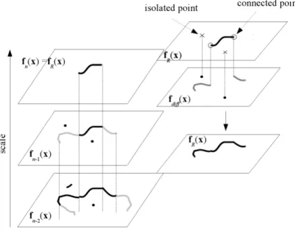
2. Project the 3D contour or surface points of the object model onto the image plane and translate the correspondence search problem completely to 2D. Essentially, information in 3D space is different than the information in the image plane. 3D features are in general not invariant against perspective projections. If only one image is used to compute the pose, 3D information can not be completely reconstructed from the image. If the 3D models are projected onto the image plane, there are more possibilities to exploit more image information and to find equivalent features from the projected models. Because of that, the second strategy is followed in order to develop the new variants of the ICP algorithm. A schematic diagram of the general strategy is presented in figure 1.1.

Fig. 1.1: General strategy to translate the correspondence problem from the 3D Eu-clidean space to the 2D image plane.

The present thesis work is organized as follows:

In chapter 2, the pose estimation problem is introduced in the framework of geometric algebras. Initially, the basic definitions and properties of geometric alge-bras are presented. The associated algealge-bras of Euclidean, projective and conformal

(23)

1.3. Contributions and Outlook 11

space are defined. Basic geometric entities like points, lines and planes as well as the image formation process are defined in projective geometric algebra. On the other hand, rigid body motions are modeled in conformal geometric algebra. Then, the interaction of these entities is described in order to define the pose estimation constraints.

The use of twist rotations as global and local contour and surface generator ele-ments is discussed in chapter 3. In a first instance, the concepts of free-form models and Fourier contour and surface approximations are introduced. Then, they are coupled with the pose estimation constraints in CGA. Additionally, contour and surface approximations are obtained from the quaternion valued Fourier transform and Hartley transform which offer an alternative to the complex valued Fourier ap-proximations for practical applications. For instance, they allow the extraction of global orientation information. By following the idea of twist rotations, a new local representation of free-form contours and surfaces in the framework of the confor-mal geometric algebra is proposed in this chapter (published in [25]). This new representation allows to generate and describe the vicinity of a model point, larger segments or even the complete model by a pivot point and a set of concatenated twist rotations. Therefore, it can be used in the pose minimization constraints de-fined by Rosenhahn. Additionally, this local representation allows to extract local features information from contour segments.

One of the central contributions of this work is presented in chapter 4. In order to extract feature information of the image, the monogenic scale space is used to detect local structure and edge information at different scales. Then, a contour search al-gorithm is applied to extract iteratively contours from the image at different scales. Based on the geometrical properties of the proposed local model representation in the image plane, a set of analog local features to that of the monogenic scale space are extracted. From the local orientation of model points, a local feature defined as transition index is presented. It represents an artificially generated structural feature analog to the local phase. Additional to these features, model and image contours are segmented according to their structure in straight, convex and concave segments. Additional constraints are defined with these features in order to define the structural ICP algorithm (published in [26]) for the case of planar 3D free-form contours.

The procedures for the contour feature extraction were extended for the case of free-form surfaces in chapter 5. Under some considerations, the local features are ex-tracted from the projected silhouette of the model with respect to the image plane. Then, the structural ICP algorithm can be applied. In contrast to the normal ICP variants, the feature information of larger contour segments is used to define pro-file vectors. Then, each contour point has an associated propro-file vector that describes its structural information. Other variant of ICP algorithm is presented in this chap-ter where the Euclidean distance is replaced by a feature measurement based on the correlation matrix defined by profile vectors of model and image points (pub-lished in [27]). For cases where the displacement between model and image data

(24)

is too large (non-tracking assumption conditions), the local orientation information is combined with the global orientation obtained from the Hartley transform in 2D. Instead of a normal pre-alignment approach, a simple feature pre-alignment in the image plane is done in order to place the model under tracking-assumption condi-tions. A set of experiments done with artificially generated data and real images are presented in chapter 6. Those experiments focus on testing of the main properties of the new variants of ICP algorithm: robustness against the tracking assumption and convergence behavior. The new ICP variants were extensively compared with the classical variants of the ICP algorithm.

In chapter 7, the problem of the pose estimation of free-form surfaces with par-tial occlusions under non-tracking assumption conditions is discussed. Additional positional features are combined with the correlation ICP algorithm as outlier elimi-nation criterion. In this case, the angular position of silhouette points with respect to its global main orientation is used. Several combinations of correspondence search criteria and outlier elimination are analyzed which have several properties and be-haviors. A system that selects the best combination according to the global position, orientation and absolute pose error is presented.

Finally, the discussion is presented in chapter 8. Several possibilities are men-tioned in order to improve the presented algorithms and to apply them to more general scenarios of the pose estimation problem.

(25)

Chapter 2 POSE ESTIMATION IN THE LANGUAGE

OF GEOMETRIC ALGEBRA

Geometric algebras have become an important mathematical framework to model geometrically related problems by focusing on the geometrical interpretation of al-gebraic entities. Prior to the introduction of the Clifford algebra, Hamilton (1805-1865) proposed quaternions as a generalization of complex numbers and applied them to model rotations in 3D space. Other important contribution is the exterior (also called outer) algebra developed by Grassman (1809-1877). In this case, the outer product of vectors is an algebraic construction that generalizes certain fea-tures of the cross product to higher dimensions. Those ideas were taken by Clifford (1845-1879) in order to develop his Clifford algebra. Essentially, Clifford made a slight modification of the exterior product (he introduced the geometric product), which allowed him to define quaternions and Grassman’s exterior algebra into the same algebraic framework.

In this chapter, an introduction to geometric algebras and the definition of the pose estimation problem in this mathematical framework are given. For a more gen-eral and detailed introduction, the reader should refer to [8, 15, 37, 85, 92, 93, 102]. Since this chapter serves as an introduction, the reader may also refer to the above mentioned bibliography for details about the presented definitions and properties. The notation and definitions used in this chapter are based on the last cited works. Initially, the geometric algebra of Euclidean space IR3 as well as its relation with the algebra of quaternions is presented. Then, the corresponding algebras of projec-tive and conformal spaces are introduced. The image formation process and basic geometrical entities (points, lines and planes) are defined in projective geometrical algebra. On the other hand, rigid body motions and operations defining points-line and point-plane incidence relations are defined in conformal geometric algebra. Fi-nally, all these concepts are used to define two different pose estimation constraints. They are based on minimization in 3D space and a projective variant based on min-imization in the image plane respectively.

(26)

2.1 Definition of Geometric Algebra

In this section, the definition of geometric algebra, its elements (multivectors) and its associated product (geometric product) are presented. A geometric algebra denoted by Gp,q,r is a linear space spanned by 2n, with n = p+q+r, basis elements

con-structed from a vector space IRp,q,r. This linear space is defined by subspaces called blades which represent elements called multivectors as higher grade entities.1 _The

indices p, q, r refer to the signature of the corresponding basis vectors. The vector space is formed byp, qandrbasis vectors which square to1,₋1and0, respectively. According to that, a proper signature can be chosen to define spaces with certain geometrical properties.

2.1.1 Geometric Product

The product operation associated with the geometric algebra is the geometric prod-uct. For two vectorsaandb, the geometric product is defined by

ab=a_·b+a_∧b. (2.1) Then, the geometric product is constructed by the combination of an inner ”_·” and an outer product ”_∧”. Let us consider the case of two orthonormal elements

ei,ej ∈ IRp,q,r of a given vector space. In general, the geometric product of these

elements leads to a scalareiej := 1 ∈ IR ifi = j. The last implies that the vectors

are the same. Otherwise, the geometric product leads to a new entity called bivector (grade two) representing the space spanned by these two vectors: eij = ei ∧ej =

−ej ∧ei ifi 6=j. These elements are the basis elements of geometric algebra. Then,

geometric algebras are expressed on the basis of graded elements.

A general multivectorMis formed by a linear combination of elements of differ-ent grades as M= n X i=0 hM_ii, (2.2)

where each element_hM_ii represents each part of the multivector with respect to its

gradei. According to that,_hM_i₀is the scalar part ofM,_hM_i₁and_hM_i₂are the vector and bivector parts respectively. If an element is constructed as the outer product of

kindependent vectors, it is called a blade of gradek. Then, the blade of the vectors

e1,e2, ...,ek is defined as

A_hki :=e1∧e2∧...∧ek. (2.3)

By using the properties of the geometric product (see [85]), it is possible to ex-press the inner and outer product of two vectors in terms of their geometric product.

(27)

2.1. Definition of Geometric Algebra 15

For two vectorsa,b_{∈ hG}p,qi1, its respective inner and outer products are defined as

a_·b := 1

2(ab+ba) (2.4)

a_∧b := 1

2(ab−ba). (2.5)

In order to clarify the operations used in the examples presented during this chapter, some rules for the computation of the inner product between blades are presented. According to [85], the inner product of a vectorx(grade 1) with a blade

A_hk_i (with gradek ≥ 1) results in a blade of gradek −1. The last can be expressed

in the next equation:

x_·A_hk_i = (x·e1)(e2 ∧e3∧e4∧. . .∧ek) −(x_·e2)(e1∧e3∧e4∧. . .∧ek) +(x_·e3)(e1∧e2∧e4 ∧. . .∧ek) −. . . = k X i=1 (₋1)i+1(x_·ei)[Ahki\ei], (2.6)

where[A_hki\ei]is the bladeAhkiwithout the vectorei.

A more general operation is the inner product of two bladesA_hk_iandB_hk_i (with

0<k _≤l _≤n). It can be computed as

A_hk_i·B_hl_i =e1· e2 ·(. . .·(ek·B_hl_i))

, (2.7)

with the resulting blade of grade l ₋k. In general, the inner product reduces the grade of a blade while the outer product increases its grade.

A generalization of the geometric product of vectors can be done for the product of general multivectors. Thus, the geometric product as the combination of inner and outer product of two vectors is extended by applying the properties or the geo-metric product (see [85]). For two general multivectors A,B _{∈ G}3, the definition of

equations (2.4) and (2.5) is used to define the geometric product as

AB = 1

2(AB+BA) +

1

2(AB−BA)

:= A_×B+A_×B, (2.8)

where the analog operators of the inner and outer products for the case of general multivectors are called commutator×and anticommutator×product respectively.

Additional to the inner and outer product, other important operations with blades are defined in the algebra. One of these operations is the reverse Ae_hki of a blade A_hk_i =e1∧e2...∧ek₋1∧ek, defined as

e

(28)

Because of the associative and noncommutative properties of the outer product, the reordering of vectors in a blade changes only its sign. Then, the reverse can be computed as

e

A_hk_i = (−1)k(k−1)/2A_hk_i. (2.10)

The reverse operation is used to define the inverse of a blade as

A−_h_k1_i:= Aehki

kA_hk_ik2

, with _kA_hkik2 6= 0. (2.11)

An important element of each algebra is the unit pseudoscalar, denoted by I, which is defined by the unit blade of highest grade. The inverse of the pseudoscalar is used to define the dual of a blade. For a bladeAof grader, the dualA∗ _{is defined}

as follows

A∗ :=AI−1. (2.12)

Ifn is the dimension of the complete space, the grade of the dual bladeA∗ will be

n₋r. Thus, the dual of a blade results in a blade complementing the whole space. An operation that evaluates the intersection of subspaces represented by blades is the ”meet”. The generalization of this operation for general multivectors is the basis to describe the camera perspective projection process and to define point-line and point-plane incidence equations. The meet operation for two arbitrary blades

A,B, denoted by the operator ”∨”, is defined as

A_∨B:= (AJ−1

∧BJ−1)J, (2.13) whereJis the result of the ”join” operator of the blades.

For two blades A and B, the join J = A ˙_∧B is defined as the pseudoscalar of the space spanned by the blades A and B (see [85] for more details). According to the last definition, the join is an adapted version of the pseudoscalar. Instead of considering the pseudoscalarIof the entire space, a ”reduced” pseudo scalar J

is constructed. For example, the join of the vector e2 with the bivector e2 ∧e3 is

simply the bivectore2∧e3. It is clear that these elements are defined in the subspace

spanned bye2∧e3. Since the vectore1 does not play any role in this example, it is

not considered in the definition of the join for this particular example.

2.2 Euclidean Geometric Algebra

In order to facilitate the reader to follow the interaction of elements in the different spaces, the following notation will be used in next sections. Points in Euclidean space will be represented with the notation x _∈ IRn. The embedding of points in projective space with X _∈ IRn+1\{0_}, while elements of conformal space will be denotedX _∈IRn+1,1_\{0_}.

(29)

2.2. Euclidean Geometric Algebra 17

Fig. 2.1: Left: outer product of two vectors expanding an oriented plane segment. Right: outer product of three basis vectors expanding an oriented segment of the complete space.

The Euclidean space, denoted by IR3, is spanned by the orthonormal basis vectors

{e1,e2,e3}. Its associated geometric algebraG3 is spanned by the following23 = 8

basis elements

G3 = span{1,e1,e2,e3,e23,e31,e12,e123}. (2.14)

As can be seen, the algebra is spanned by one scalar, there vectors (e1,e2,e3),

three bivectors (e23,e31,e12) and a trivector (e123) . This trivector is also known as

unit pseudoscalar (IE). It squares to -1 and commutes with all other elements of the

algebra.

A multivectorM_{∈ G}3 is the combination of all these basis elements:

M= a0+ a1e1+ a2e2+ a3e3+ a4e23+ a5e31+ a6e12+ a7e123. (2.15)

The geometrical interpretation of these elements can be seen in figure 2.1. The outer product of two vectors defines the area of the parallelogram formed by them. Then, the outer product represents the oriented segment of a plane spanned by these two vectors (the orientation is represented by the arrows in the figure). In a similar way, the outer product of three basis elements represents the oriented unit volume and therefore a segment of the complete space.

Geometrically, the inner and outer products serve as operators that increase or decrease the grade of a given blade or multivector. While the outer product of two blades results in a blade of higher grade, the inner product decreases its grade. By following the definition of equation (2.6), the result of the inner product of the bivec-tore1 ∧e2with the vectore1is

e₁_·(e1∧e2) = (e1·e1)e2−(e1·e2)e1 =e2.

Sincee1·e1 = 1ande1·e2 = 0are scalars, it is clear that the outer product of a vector

(30)

can be interpreted as a ”subtraction” of the subspace spanned bye1 from the space

spanned bye1∧e2.

It has been shown in [92] that the dual operation of a blade defined in equation (2.12) plays an important roll to construct an algebraic representation of points, lines and planes based on their geometrical representations. This will be described in the next sections. Let us consider one of the examples presented in [85] in order to clarify how the dual works in Euclidean geometric algebra. As described before, the bivectore2∧e3 describes a plane. By the definition of equation (2.12) and according

to the inner product rules of equations (2.6) and (2.7), it follows that

(e2∧e3)∗ = (e2∧e3)·I−E1

= (e2∧e3)·(e3 ∧e2∧e1)

= e₂_·[e₃_·(e₃_∧e₂_∧e₁)]

= e2·[(e3 ·e3)(e2∧e1)−(e3·e2)(e3∧e1) + (e3·e1)(e3∧e2)]

= e2·[e1∧e2]

= e1. (2.16)

It is clear that the vector e₁ is the dual element of the plane e₂ _∧ e₃. On the other hand, let us remember how to represent a plane in the Euclidean space IR3. According to the Hessian representation of a plane, it is described by the normal unit vector of the plane and the distance from the origin to the plane. As can be seen in the last example, the result of the dual operation provides the normal vector

e1 which is also used by the Hessian representation. The Hessian representation

describes a plane only in IR3. In contrast to that, the bivector or its dual always describe a plane independent of the dimension of the space they are embedded in. This simple example gives a hint of how the dual operation can provide an algebraic element which can be used to represent a geometrical entity. As it will we shown in the next sections, the dual operator is used to find dual representations of points, lines and planes which can be embedded from projective to conformal space and viceversa.

2.2.1 Quaternions

In this section, the ideas presented in [85] to define an isomorphism between quater-nions and geometric algebras are summarized. In the next chapter, quaterquater-nions will be used as an alternative to model 3D free-form objects as a combination of rotations in the context of geometric algebras.

Quaternions are a non-commutative extension of the complex numbers. They are defined by the combination of a scalar with three imaginary componentsi,jand

(31)

2.2. Euclidean Geometric Algebra 19 ksatisfying the following rules

i2 =j2 =k2 =₋1, ij=k, jk=i, ki=j

ij=₋ji, jk=₋kj, ki=₋ik, ijk=₋1. (2.17)

A general quaternionqhas the formq= q0+q1i+q2j+q3kwithq0,q1,q2,q3 ∈IR.

A quaternion which does not have a scalar component is called a pure quaternion

p = q1i+ q2j+ q3k. The complex conjugate of a quaternion qis denoted by q∗ =

q0 − q1i − q2j − q3k. Similar to the complex numbers, a quaternion can be also

expressed in exponential form as

q = rexp(θp)ˆ , (2.18) wherer =√qq∗_,_θ _{= atan(}√pp∗

q0 )andpˆ =

p

√

pp∗. The exponential representation of a

unit quaternion can be interpreted as a rotation operation. A vector represented by the pure quaternionais rotated by the following operation

b = r a r∗, (2.19)

withr = exp 1₂θˆpandpˆthe unit quaternion representing the rotation vector. Then, the vectorais rotated by an angleθaround the vector represented bypˆ.

Since quaternions are formed by a combination of a scalar component and three imaginary components, an isomorphism can be defined between quaternions IH and geometric algebra. The key idea of this isomorphism is that bivectors ofG3 have the

same properties as the imaginary quaternion unitsi, j and k. Thus, the imaginary units can be identified with the following bivectors:

i_→e₂₃, j_→e₁₂, k_→e₃₁. (2.20) Then, quaternions can be considered as elements of the subalgebra _G₃+ _{⊂ G}3

spanned by the basis vectors:

G+

3 = span{1,e23,e12,e31}. (2.21)

Since the subalgebra_G3+is isomorphic to the quaternion algebra IH, all properties

of equation (2.17) are valid for the bivectors defining G3+. By using the geometric

product, it ha been shown in [85] that the known relations between the imaginary units are preserved,

ij_→(e2e3)(e1e2) = (e3e1)→k , (e3e1)2 =−1

jk_→(e1e2)(e3e1) = (e2e3)→i , (e2e3)2 =−1

ki _→(e3e1)(e2e3) = (e1e2)→j , (e1e2)2 =−1.

(32)

Let us consider the rotation operation of equation (2.19) with the unit quaternion

ˆ

p = x1i+x2j+x3kdefining the rotation axis. According to the basis identification

of equation (2.20), this unit quaternion can be directly related to the unit bivector

n=x₁e₂₃+x₂e₁₂+x₃e₃₁_{∈ G}₃+. Then, the analog rotation operation called ”rotor” of equation (2.19) can be written as

R= exp

−1₂θn

∈ G3+. (2.23)

Notice thatpˆ represents a rotation vector in IH whilenrepresents a plane in_G3+.

That means, the rotation is performed around a rotation axis in IH while the same rotation is performed with respect to a plane in_G₃+.2 _Although_n_and_p_ˆ_{are different}

geometrical entities defined in different algebras, there is a relation between their parameters. To make this idea clear, the dual operation is applied to the bivectorn. Similar to the example of equation (2.16), the dual of each basis element ofnare

(e2e3)∗ =e1, (e1e2)∗ =e3, (e3e1)∗ =e2.

Therefore, the dualn∗ =x₁e₁+x₂e₃+x₃e₂ corresponds to the rotation vector repre-sented by the unit quaternionx1i+x2j+x3kaccording to the identification of equation

(2.20). If quaternions are used to represent vectors in Euclidean space, each imag-inary uniti,j and kis identified with the three x, y and z axes respectively. In G3

these axes are denoted by e1, e2 and e3. Notice that the axes e2 and e3 of n∗ are

changed. Then, the corresponding change of axes produces the change of sign in the rotation of equation (2.23).

One advantage of using rotors over quaternions is that rotors can be defined in any dimension. While rotations can be only applied to vectors in quaternion algebra IH, rotations in_G₃+can be applied to blades of any grade e.g. lines and planes.

2.3 Geometric Algebra of Projective Space

Essential for the pose estimation problem is the representation of basic geometric entities like points, lines, planes as well as their interaction with the image formation process. This is not possible in Euclidean geometric algebra _G3. Therefore, the use

of projective geometry is required.

The projective space IPIRn (with dimension IRn+1\{0_}excluding the origin) is de-fined by all elementsXandY, which form a set of equivalence classes∼such that

∀X,Y_∈IPIRn :X_∼Y _{⇔ ∃}λ_∈IR_\{0_}:X =λY. (2.24)

2_{This fact is the principle for the construction of rotations in geometric algebra that will be}

(33)

2.3. Geometric Algebra of Projective Space 21

The projective space is illustrated in figure 2.2 for IR2. All the points of the line defined byXand the origin represent the same point in the projective plane. Thus, the entire equivalence class is collapsed into a single object, for this example in a single point. The basis elements of projective space are the orthonormal vectors

{e₁,e₂, . . .en,en+1}, where the basis vector en+1 is known as homogeneous

compo-nent.

The operatorsP and P−1 _{are defined in [85], which denote the transformations}

of an element from Euclidean (x_∈IRn) to projective space (X_∈IPIRn) and vice versa as P(x) = x+en+1 ∈IPIRn (2.25) P−1(X) = 1 X_·en+1 n X i=1 (X_·ei)ei ∈IRn. (2.26)

As can be seen in the last equation, the homogeneous component of X is always the unity. These transformations are illustrated in figure 2.2.

Then, the Euclidean space IR3 is embedded in projective space IPIR3 by adding a homogeneous component denoted by e₋, with the property that e2₋ = ₋1. The corresponding geometric algebra of projective space_G3,1is spanned by the following

24 _{= 16}_elements

G3,1 = span{1,e−,e1,e2,e3,e23,e31,e12,e−1,e−2,e−3,

e123,e−23,e−31,e−12,e−123},

(2.27)

with the pseudoscalarIP :=e−123with the property that withe2₋123 =−1.

The outer product is important in the definition of the projective geometric alge-bra. It has been discussed in [87] that the outer product is used to define the equiva-lence class of equation (2.24). SinceX_∧X= 0, it is clear thatX_∧λX= 0_∀λ_∈IR_\{0_}. Hence, all vectorsXrepresent a pointAifA_∧X = 0.

2.3.1 Points, Lines and Planes in Projective Geometric Algebra

The idea of representing a point in projective space is shown in the left graphic of figure 2.2 for IR2. Because of the homogeneous representation ofX_∈IPIR2, all points along this vector excluding the origin represent the same point x _∈ IR2. A point

x = x1e1+ x2e2 + x3e3 ∈ G3 is represented in projective geometric algebraG3,1 just

by adding the homogeneous coordinatee₋as

X =x+e₋= x1e1+ x2e2+ x3e3+e−. (2.28)

The right graphic of figure 2.2 shows the idea of representing lines. Let us consider two points x1,x2 ∈ IR2 and their respective homogeneous vectors X1,X2 ∈ IPIR2.

(34)

Fig. 2.2: Left: example of the embedding of an Euclidean vector in projective space and the opposite projection of a homogeneous vector to Euclidean space. Right: representation of a line in projective space by two homogeneous vectors.

Then, a plane is spanned by these homogeneous vectors (see [85]). The points that result from the intersection of this plane with the projective plane define a line in IPIR2. As can be seen in the figure, this line does not pass through the origin. Finally, the orthographic projection of the intersection gives a line in IR2.

In order to define lines and planes in projective geometric algebra, the outer product of points is used as defined [92]. Let us consider the case of a lineL _{∈ G}3,1. It

is obtained by the outer product of two pointsX1,X2. This operation in the algebra

to obtain a line is summarized as described in [92] as follows

L = X1∧X2

= (x1+e−)∧(x2 +e−) = x1∧x2 + (x1−x2)e− = m₋re₋,

(2.29)

where the parametersm(moment) and r (direction) are same parameters used by the Pl ¨ucker representation of a line [15].

Similarly, a plane in projective space is represented by the outer product of three pointsX1,X2,X3 ∈ G3,1. This operation is summarized as presented in [92] as

fol-lows P = X1∧X2∧X3 = (x1+e−)∧(x2+e−)∧(x3+e−) = x1∧x2∧x3+ (x1−x2)∧(x1−x3)e− = dIE +ne−. (2.30)

(35)

2.3. Geometric Algebra of Projective Space 23

Fig. 2.3: Left: coordinate systems involved in the complete camera model. Right: definition of the image plane according to the normalized camera model. In this case, the parametersn(normal of the plane) andd _∈IR (distance to the ori-gin) are the parameters used in the Hesse representation of planes. In comparison with the elements of the algebra of Euclidean space G3, algebraic linear

represen-tations are gained from the basic geometrical concept of construction of lines and planes: two points define a line and three points a plane.

2.3.2 Camera Model in Projective Geometric Algebra

The pinhole camera model defines the perspective projection of spatial points onto the image plane. More detailed information about the pinhole camera model can be found in [37]. For a given number of world points and their corresponding im-age points, the calibration matrix defining the projection is computed. Additionally, it can be can decomposed in a set of external and internal parameters (known as complete camera model, see [45]). As shown in figure 2.3, this set of parameters defines the relation between the different coordinate systems involved in the pro-jection process: world _Ow, camera Oc and image Oim. In the next equations, the

corresponding origin points of these coordinate systems are denoted asOw,Oc and

Oim respectively. The external parameters are encoded in the matrix Mext which

defines the rigid body motion needed to represent a point in the camera coordinate system. From this matrix, the location of the optical center of the cameraOc can be

obtained. The internal parameters are defined by the scale factorsf ku, f kv in theu

andv image axes directions and the coordinates of the principal point in the image

(u0, v0). The principal point is the point where the optical axis intersects the image

plane (note that this point may not necessary be the center of the image). Based on these parameters, a pointXn ∈ IPIR3 is projected onto the image plane in two steps.

First, it is transformed to the camera coordinate systemX′

n =x1e1+x2e2+x3e3+e−

by the rigid body motion Mext. Finally, it is projected onto the image plane by the

internal parameters to the point

Ximg_n = _fk ux1 +u0 x3 e1+ _fk ux2+v0 x3 e2+e3+e−∈ G3,1. (2.31)

(36)

The camera model is constructed and normalized in such a way, that the image center intersects the optical axis at the point with coordinates(0,0,1)in the camera coordinate system_Oc(notice that its origin point corresponds to(0,0,e3)). Since the

uandv image axes are parallel to the basis vectorse₁ande₂ respectively, the image plane is spanned in projective space by the points

X1 = αe3+e− ∈ G3,1

X₂ = α(e1+e3) +e− ∈ G3,1

X3 = α(e2+e3) +e− ∈ G3,1,

(2.32)

with the factorα _≥ 1_∈ IR. Notice that the exact position of the image plane can be found since the internal and external parameters are known.

It is possible to define the perspective projection of equation (2.31) as the result of intersection of the image plane and a line defined by the point and the optical center. Then, the image plane is defined according to equation (2.30) by the outer product of the pointsX1,X2andX3 as

Pim = X1∧X2∧X3

= e₃_∧(e1+e3)∧(e2+e3) + (e3−(e1+e3))∧(e3−(e2+e3))∧e− = ₋e1∧e2∧e3+ (e1∧e2)e−

= ₋IE + (e1∧e2)e−. (2.33)

Since the optical center is considered as the origin of the coordinate system, it has the form Oc = 0 +e₋ ∈ G3,1. The line defined from the optical center and the

pointXn =xn +e−∈ G3,1is computed according to equation (2.29) by

Ln = xn∧0 + (xn−0)e−

= xne−. (2.34)

According to equation (2.13), the intersection of this line and the image plane is computed by the meet operation ”_∨”

Ximg n = Ln ∨Pim = (Oc∧Xn)∨(X1∧X2∧X3) = (₋IE + (e1∧e2)e−)∨(xne−) = p1e1+p2e2+e3+e−. (2.35)

To find its corresponding pixel coordinates in the image, the internal camera pa-rameters are used as it was shown in equation (2.31) to scale the point coordinates as follows