A theory of contractual provisions in leasing
Thomas Chemmanur
a,*,1, Yawen Jiao
b, An Yan
ca
Carroll School of Management, Boston College, Chestnut Hill, MA 02467, USA b
Lally School of Management and Technology, Rensselaer Polytechnic Institute, Troy, NY 12180, USA c
School of Business Administration, Fordham University, New York, NY 10023, USA
a r t i c l e
i n f o
Article history:
Received 24 October 2005 Available online xxxx
a b s t r a c t
We develop a non-tax rationale for leasing in a double-sided asym-metric information setting, and analyze how various contractual provisions in leasing contracts arise in equilibrium. In our model, a manufacturer of capital goods has private information about their quality; entrepreneurs (users of these capital goods) come to learn this quality only by using them over a period of time. Each unit of the capital goods requires a certain level of maintenance in each period. Entrepreneurs differ in their cost of providing this mainte-nance; this maintenance cost is information private to each entre-preneur. Leasing emerges as an equilibrium solution to this double-sided asymmetric information problem. Various contrac-tual provisions in leasing contracts (e.g., short-term versus long-term leases with non-cancellation provisions, option to buy at lease termination, and service leases) also emerge as equilibrium solutions under alternative settings. Leases with metering provi-sions emerge in equilibrium when, in addition to the maintenance cost, entrepreneurs differ in other dimensions, such as their inten-sity of usage of the capital good. Our model has implications for the lease-versus-sell decision, the situations under which various leas-ing contract provisions will be used, and for the relative magni-tudes of sales prices and leasing costs (for leases with different contractual provisions).
Ó2009 Elsevier Inc. All rights reserved.
1042-9573/$ - see front matterÓ2009 Elsevier Inc. All rights reserved. doi:10.1016/j.jfi.2007.09.002
*Corresponding author. Fax: +1 617 552 0431.
E-mail addresses:[email protected](T. Chemmanur),[email protected](Y. Jiao),[email protected](A. Yan).
1 Thomas Chemmanur acknowledges support from Boston College Faculty Research Grant, and An Yan acknowledges support from Fordham University Faculty Research Summer Grant. For helpful comments or discussions, we thank the editor, S. Viswanathan, two anonymous referees, Ingela Alger, Richard Arnott, Paolo Fulghieri, James Schallheim, and Fabio Schiantarelli, as well as participants at the Western Finance Association meetings, the Financial Management Association meetings, and seminars at Boston College and Fordham University. We alone are responsible for any errors or omissions.
Contents lists available atScienceDirect
J. Finan. Intermediation
j o u r n a l h o m e p a g e : w w w . e l s e v i e r . c o m / l o c a t e / j fi1. Introduction
Leasing is an important source of external financing for U.S. corporations. It has been estimated that a third of the capital equipment used by U.S. corporations is leased. However, the motivations for leasing are still not completely understood. While the finance literature has analyzed corporate leasing policy extensively, much of the discussion has been confined to tax-related incentives to lease or buy (see, e.g.,Miller and Upton, 1976; Lewellen et al., 1976). These and other papers assume that the real operating cash flows associated with leasing or owning are invariant to the financial contract chosen, thus assuming that it is primarily tax-related incentives which drive the lease or buy decision. More recently, however, financial economists have come to recognize that, while taxes are impor-tant in determining the identity of the lessor and the lessee, they may be less crucial in identifying the specific assets to be leased. The co-existence of both leased and purchased assets suggests that the net benefits of leasing may be neither uniformly positive nor negative. The predominance of leasing in cer-tain industries and for cercer-tain assets implies wide variations in the benefits from leasing. Equally important is the variety of contractual provisions observed in practice, based on service provisions, option to cancel the lease before the maturity of the contract or to renew it for additional periods, op-tion to buy the asset at the terminaop-tion date of the lease, metering, etc. To illustrate, consider the example of a hospital leasing medical equipment (e.g., MRI or CT systems). When the equipment’s lease has ended, the hospital has several options: return the equipment to the lessor, and replace it with newer equipment that better meets the hospital’s needs; renew the lease for an additional per-iod; or buy the equipment as used equipment at its fair market value. Clearly, tax considerations offer little explanation for the inclusion of such contractual provisions in the above and similar situations. The objective of this paper is 2-fold. First, we develop a non-tax rationale for leasing in an asym-metric information framework and analyze the lease-versus-buy decision in such a setting. Second, we develop a theory of contractual provisions in leasing in the above asymmetric information environ-ment. In particular, we analyze the following question: Under what conditions are different kinds of leasing (as well as sales) contracts offered in equilibrium? We show that, depending upon the nature of the capital equipment and the characteristics of the lessor and the lessee, the following leasing con-tract provisions emerge in equilibrium: short-term and long-term operating leases (with non-cancel-lation provisions); leases which grant the lessee an option to buy the asset at a pre-specified price at the termination date; service leases, where the manufacturer agrees to maintain the equipment leased; and leases involving metering, where the lease payment is a function of an observed measure of the intensity of usage of the asset.
We develop our model in a setting of asymmetric information where the manufacturer of capital equipment (lessor) has private information about the intrinsic value (type) of the asset he leases to the entrepreneur (lessee). The entrepreneur, however, can learn more about the value of the equip-ment over time as she uses the asset. We assume that entrepreneurs (lessees) are also heterogeneous. This heterogeneity can be in their cost of maintaining the leased equipment (as in our basic model) or in their intensity of usage of the leased equipment (as in Section5.2). We assume that entrepreneurs have superior information compared to manufacturers about their cost of maintenance (or usage intensity, in Section5.2).2While all entrepreneurs have some incentive to maintain the equipment (since the condition of the equipment affects the future profits it can generate for entrepreneurs), this incentive is weaker for higher maintenance cost entrepreneurs than for lower maintenance cost entre-preneurs. We demonstrate that, in this setting, the decision by a manufacturer regarding whether to offer his capital equipment under a leasing or a sales contract, as well as the contractual provisions in the leases he offers, allows him not only to reveal the true quality of his equipment, but also to segment the market for capital equipment among different kinds of entrepreneurs, thus maximizing his profit.
In equilibrium, high type manufacturers choose to lease their capital equipment to entrepre-neurs, while lower type manufacturers choose to sell the equipment outright. Manufacturers are aware that entrepreneurs will learn the true type of the leased equipment after using it for some
2
In other words, our setting is one of contracting under double-sided asymmetric information, where both the manufacturer (lessor) and the entrepreneur (lessee) have some (private) information not available to the other party.
time, and will renew the lease if the value of the equipment to them is high, while returning lower value equipment to the manufacturers (who receive the residual value of the equipment). Conse-quently, while manufacturers of high value equipment are better off leasing their equipment, those of low value equipment are better off selling them outright at the price reflecting their true value. At the same time, manufacturers of high value equipment are able to segment the capital equip-ment market between the two kinds of entrepreneurs by offering leases with different contractual provisions. In one situation (analyzed in Section4.1), this is achieved by offering a combination of a short-term and a long-term (non-cancellable) operating lease: in equilibrium, lower maintenance cost entrepreneurs will choose the short-term leasing contract and purchase the equipment at the end of the initial leasing period, while higher maintenance cost entrepreneurs will choose the long-term leasing contract but will return the equipment to the manufacturers at the end of the initial leasing period (i.e., they will not purchase the equipment at the end of the lease). In other situations (Section5.1), manufacturers may make use of leases with service provisions to segment the leasing market: they may offer leases with and without service provisions. In this case, higher maintenance cost entrepreneurs will accept leases with service provisions in equilibrium, while lower maintenance cost entrepreneurs will accept leases without such provisions. Similarly, in Sec-tion5.2, we demonstrate that manufacturers may use metering provisions in leases to distinguish between entrepreneurs with a high-intensity of usage and those with a low-intensity of usage of the capital equipment: in equilibrium, low-intensity entrepreneurs accept leases with metering while high-intensity entrepreneurs accept leases without metering.
The rationale for leasing developed here is particularly relevant to the leasing of capital equip-ment making use of newer technologies, which is more likely to be characterized by asymmetric information. In a survey of entrepreneurs by the Small Business Administration (SBA), regarding the motivations that led them to lease instead of purchasing capital equipment, 13% cited the abil-ity to access the latest technology in the least risky way as the main motivation; another 13% mentioned maintenance options and costs. In contrast, only 9% mentioned tax-advantages as the main motivation behind leasing.3 Further, one of the important motivations for leasing often given
by practitioners is that leasing equipment allows technological risk (i.e., the risk that equipment using new technologies may not be appropriate for the use at hand, or the risk of technological obso-lescence) to be transferred from the lessee (entrepreneur) to the lessor (manufacturer).4However, it
is not obvious how such a transfer of technological risk can create value if both lessors and lessees are corporations (and therefore essentially risk-neutral). In this paper, we demonstrate that such a transfer of technological risk through leasing can indeed create value in an environment of asymmet-ric information: i.e., in a setting where lessors have more information, compared to lessees, about the quality of their capital equipment (and its underlying technology). Our model generates several implications for the prevalence of leasing contracts relative to sales contracts, the contractual provi-sions in leasing contracts, as well as for the relative magnitudes of leasing costs and sales price to users of the capital equipment.
Our research is related to several strands in the finance and economics literature. As mentioned be-fore, there is a large finance literature on leasing focused on tax-related incentives to lease or buy. However, tax issues alone cannot explain the existence of leasing in many markets: while the tax ben-efits of leasing were lowered in the tax reform act of 1986, the importance of leasing has increased. Neither can tax arguments explain the existence of the variety of leasing contracts observed in prac-tice.Smith and Wakeman (1985)provide an informal but insightful analysis of the determinants of corporate leasing policy. They argue that leases can reduce the transaction costs that arise when the physical life of the asset exceeds the economic life of the firm, and informally discuss several pos-sible rationales for some of the common provisions in leasing contracts.Sharpe and Nguyen (1995)
3
A significant percentage of entrepreneurs also gave cash flow constraints as the reason for leasing. In another survey conducted by Dun and Bradstreet of the top five reasons for choosing to lease, 18% chose rapid technological change as the main reason for leasing (see,Gerety, 1995).
4
This particular quote was taken from the web site of the Equipment Leasing Association. Similar quotes occur frequently again in the practitioner literature and practitioner surveys.
hypothesize that firms facing high financial contracting costs can alleviate these costs by leasing, and present evidence indicating that such firms have a high propensity to lease.5
Hendel and Lizzeri (2002) and Johnson and Waldman (2003)develop a theoretical analyses of leas-ing contracts focusleas-ing on the relationship between the new car market and the used car market. Hen-del and Lizzeri (2002)study a setting where there are two types (levels of quality) of cars, with consumers having heterogeneous valuations for quality. To begin with, neither the manufacturer nor consumers know the true quality of a new car, so that there is no adverse selection in the new car market. However, consumers can observe the quality of a car through using it over time, so that the used car market is characterized by adverse selection. A leasing contract in their setting specifies not only the rental payment for the car, but also the option price at which a consumer can purchase the car at lease maturity. In the above setting, they demonstrate two important results. First, leasing and selling can co-exist in the new car market: consumers with a high valuation for quality prefer to lease a car while those with a low valuation prefer to buy. Leasing thus allows the manufacturer to increase profits by segmenting the new car market between the two kinds of consumers. Second, con-sumers who observe that their leased cars are of a low quality return them to the manufacturers, while those observing a high quality purchase their cars at the buyback (or option) price. The latter result implies that the manufacturer can set the option price specified in the lease for a new car above the market clearing price in the used car market (to reflect the higher quality of off-lease cars). The analysis ofJohnson and Waldman (2003)also generates results broadly similar to that ofHendel and Lizzeri (2002). While, like our paper, the above two papers also demonstrate that the manufac-turer’s expected profit can be increased through leasing, the motivation for leasing in these papers is quite different from that in our paper (recall that, in these papers, the manufacturer of a new car does not have any private information about its quality). In particular, the signaling role of leasing, the primary focus of our paper, has not been explored before in the literature. Further, the above two papers do not incorporate differences in maintenance costs across lessees and therefore do not study the role of leases in separating high maintenance cost lessees from those with low maintenance costs.6Finally, neither of the above papers analyzes the rich menu of contractual provisions present in
real-world leasing contracts.7
Our paper is also related to the contemporaneous paper byEisfeldt and Rampini (2009), who argue that, in the event of financial distress, Chapter 11 of the U.S. bankruptcy code makes it easier for a financier to repossess equipment that is leased compared to obtaining control of the same piece of equipment if it were used to secure a loan. Therefore, the debt capacity of leasing exceeds the debt capacity of secured lending, since leasing allows a financier to extend more credit to a financially con-strained firm relative to the case where he makes a loan to the firm.8Finally, from a technical
perspec-tive, our paper is also related to the literature on warranties (see, e.g.,Grossman, 1980) which has analyzed how warranties can signal product quality in a setting where the manufacturer has private information about quality. It is also broadly related to the industrial organization literature on price dis-crimination under incomplete information (seeTirole, 1999, Chapter 3 for a review), and contributes to this literature as well.
The rest of the paper is structured as follows. Section2describes the structure of our basic model. Section3discusses the benchmark outcomes. Section4characterizes the equilibrium in this model. Section5extends a simplified version of our basic model and analyzes service leases (Section5.1)
5
Other papers which lend support to the argument that leasing reduces contracting costs in various settings areKrishnan and Moyer (1994)andBarclay and Smith (1995).
6
See, however, the contemporaneous paper byJohnson and Waldman (2004), who incorporate the moral hazard problem in maintenance in a setting otherwise similar toJohnson and Waldman (2003).
7
McConnell and Schallheim (1983)value various provisions in leasing contracts using the redundant-assets methodology of option pricing models. However, since they use the arbitrage-free option pricing methodology, they, by definition, do not study issues of the optimality of these provisions. Two other papers which take a valuation approach to leasing contracts are those by
Grenadier (1995, 1996). 8
Two other arguments for leasing from the economics literature are provided byBulow (1986), who argues that leasing can be used by a monopolist to overcome the Coasian time-inconsistency problem, and byWaldman (1997), where leasing is used by a durable goods manufacturer with significant market power to eliminate the second-hand goods market. See alsoGavazza (2005), who argues that the rationale for leasing arises from lessors having a transaction cost advantage in redeploying capital.
and leases with metering (Section5.2). Section6discusses the implications of the model and Section7 concludes. The proofs of various propositions, as well as the definitions of various threshold values in these propositions, are confined to the appendix.
2. The basic model
The model has four dates (three periods). At time 0, a risk-neutral entrepreneur requires one unit of a capital good (equipment) to implement a positive net present value project. Capital equipment is produced by risk-neutral manufacturers who have private information regarding their type. Type G capital equipment generates greater cash flows for entrepreneurs than type B capital equipment (details of these cash flows will be discussed later). We can think of the type of a piece of capital equip-ment as any variable (or combination of variables) affecting the cash flows it can generate for users, and about which the manufacturer has private information. One such variable is the true quality of the equipment, which can affect its probability of breakdown, and thereby the cash flows it can gen-erate for users. Another variable is the manufacturer’s own future rate of introduction of new prod-ucts, which, in turn, will affect the rate of technological obsolescence of the capital equipment and thereby its value to users. At time 0, the entrepreneur is unable to distinguish between type G and type B capital equipment. She only knows the prior probability distribution of equipment type: she believes the equipment (manufacturer) of type G with a probabilityhand of type B with the comple-mentary probability 1h.
The entrepreneur may buy or lease the capital equipment from the manufacturer. And the manu-facturer may offer more than one kind of leasing contract to the entrepreneur (e.g., a short-term or a long-term lease). We will discuss the contract structure in more detail below.
The entrepreneur has private information about her own type. In the basic model, we assume that the entrepreneur’s private information is about her cost of maintaining the capital equipment per per-iod.9The type L (low-cost) entrepreneur has a lower costc
Lof maintaining the equipment in each period
than the type H (high-cost) entrepreneur whose maintenance cost per period iscH,cH>cL. We denotec
by the difference in the maintenance cost between the type H and type L entrepreneurs;ccHcL. At
time 0, before observing the contracts accepted by entrepreneur, the manufacturer is unable to distin-guish between the two types of entrepreneurs, so that he only has a prior probability distribution over entrepreneur types: he believes that an entrepreneur is of type H with a probability/and of type L with the complementary probability 1/.
Between time 0 and time 1, i.e., in the first period, as the entrepreneur uses the capital equipment, she receives additional information about the type of the capital equipment. For simplicity, we assume that this information is not noisy, i.e., the entrepreneur comes to know the true type of the capital
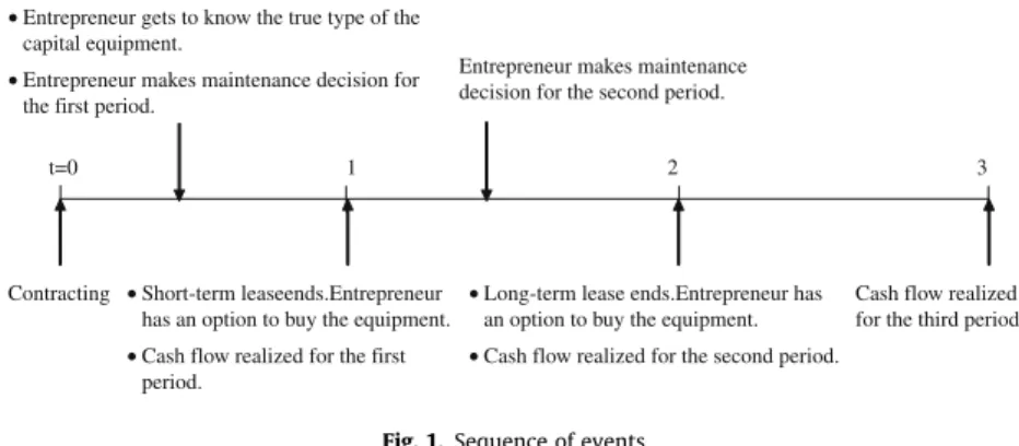
t=0 1 2 3
Contracting •Short-term leaseends.Entrepreneur has an option to buy the equipment.
•Cash flow realized for the first period.
•Entrepreneur gets to know the true type of the capital equipment.
•Entrepreneur makes maintenance decision for the first period.
Entrepreneur makes maintenance decision for the second period.
•Long-term lease ends.Entrepreneur has an option to buy the equipment.
•Cash flow realized for the second period.
Cash flow realized for the third period.
Fig. 1.Sequence of events.
9
equipment at this time. After the arrival of this information, the entrepreneur decides whether to per-form maintenance for the first period. The entrepreneur makes a similar maintenance decision in the second period as well. In addition, the entrepreneur has other choices to make depending on the terms of the type of leasing contract she accepts. If the entrepreneur chooses a short-term lease, she chooses whether or not to buy the equipment at time 1. On the other hand, if the entrepreneur chooses a long-term lease at time 0, she has the option to buy the equipment at time 2. At time 3, the project ends, and the final cash flows from the project are realized. The sequence of events is summarized inFig. 1. We normalize the risk-free rate of return to be zero.
2.1. Cash flow structure
If the equipment is well-maintained (i.e., in good condition), the type G equipment will yield a cash flow ofxin each of the three periods for which it is utilized for the entrepreneur’s project. For the type B equipment, the corresponding cash flow per period will only befx,f< 1. (We will often refer tofas the quality factor capturing the difference in value between the two types of equipment, for a given level of maintenance.) If the equipment is not well-maintained, the cash flow generated by the equip-ment will decline by a fraction of 1din the next period. We assume throughout the paper thatd< 1. We considerdas a damage factor gauging the damage sustained by the equipment due to a lack of maintenance. For example, if the equipment is not well-maintained in the first period, the cash flow in the second period will bedxinstead ofxfor the type G equipment; this cash flow will befdxfor the type B equipment. We assume that the useful life of either type of equipment is three periods, so that the equipment cannot generate any cash flows to the entrepreneur (or the manufacturer, if the equip-ment is returned to him) after time 3.
For tractability, we assume thatfis sufficiently small such that (1d)fx<cL. This assumption
im-plies that the cash flow from the type B capital equipment is such that it is not optimal to maintain the type B equipment even for the type L entrepreneur (as well as the type H entrepreneur). We also as-sume thatcL< (1d)x, so that it is optimal for the type L entrepreneur to maintain the type G capital
equipment. Note that whether or not the type H entrepreneur finds it optimal to maintain the type G equipment depends onc, the difference in maintenance cost between the type H and the type L entre-preneurs. Ifcis sufficiently large so thatcH> (1d)x, then it is not optimal for the type H entrepreneur
to maintain the type G equipment at all.
The entrepreneur has an option to return the equipment to the manufacturer at the end of the lease (if she does not choose to renew the lease). We assume that, if the entrepreneur returns the equip-ment, she receives zero cash flow for each period and the manufacturer owns the residual value of the returned equipment. We assume the following about the residual value of capital equipment.10 First, we assume that it is the entrepreneur who can put any piece of new or well- maintained equipment to its most productive use, so that the residual value of any piece of well-maintained type G equipment will be less than its value to either a type H or a type L entrepreneur.11On the other hand, for type G
equipment that is not well-maintained (i.e., for older equipment for which maintenance has not been performed in the previous period), our assumption is that its residual value isbtimes the present value of future cash flows that would be generated by the equipment by a type H entrepreneur,b> 1. In other words, for type G equipment that is not well-maintained, its residual value to the manufacturer will be
10
The residual value can arise in many ways. One possibility is that the manufacturer is able to put the capital equipment to some alternative use for himself. Another possibility is that there exists a second-hand market for the capital goods which can be used by the manufacturer to dispose of any units of the capital goods which are returned to him by entrepreneurs.
11
This assumption implies that all manufacturers have an incentive to lease out their equipment for at least one period, regardless of the maintenance cost of the entrepreneur leasing the equipment (rather than retaining the equipment themselves starting from time 0). Recall that the only difference between type H and type L entrepreneurs in our setting is their cost of maintaining equipment, so that the two are equal in their productive capacity on a well-maintained equipment. Thus, the residual value of a piece of well-maintained equipment cannot exceed its value to a type H or a type L entrepreneur.
greater than its value to a type H entrepreneur.12Finally, for simplicity, we assume that the residual
va-lue of type B equipment to its manufacturer is zero at any date.13 2.2. Contract structure
In the basic model, we allow the following menu of contracts between the manufacturer and the entrepreneur: a sales contract, where the entrepreneur pays the sales priceSup-front (at time 0) and possesses the ownership of the equipment for the entire useful life of the equipment, i.e., for all three periods; a short-term leasing contract with an option to buy {M, R}, where the entrepreneur pays the initial leasing priceMup-front and has an option to buy the equipment at time 1 by paying a purchase priceR; and a long-term leasing contract with an option to buy {N, P}, where the entrepre-neur leases the capital good for two periods (i.e., till time 2) by paying the initial leasing priceN up-front, with an option to buy the equipment by paying a purchase pricePat time 2.14We will introduce
two additional types of leasing contracts, namely, service leases and leases with metering in Sections5.1 and 5.2, respectively.
Of the above menu of contracts, the set of contracts actually offered will be determined in equilib-rium: i.e., not all contracts will be offered in all situations.15We assume that the manufacturer first
chooses the set of contracts to be offered to the entrepreneur from the above menu (at time 0). Then, after observing the contracts offered, the entrepreneur chooses the contract to accept and makes further decisions about the capital equipment over time according to the options specified in the contract accepted.
2.3. The manufacturer’s objective
The objective of the manufacturer in choosing the menu of contracts (including contract provisions, as well as prices) to be offered to entrepreneurs is to maximize the expected value of his future cash flows. Consider the objective of the type G manufacturer. If the type G offers a short-term leasing contract with an option to buy {M, R}, his expected payoff is:
P
GðSTÞ ¼MþIHST/Rþ 1I H ST /bðdxþd2xÞ þIL STð1/ÞRþ 1I L ST ð1/Þbðdxþd2xÞ: ð1Þ 12For example, if a type H entrepreneur returns the equipment to the type G manufacturer at time 1 without performing maintenance in the previous period, the residual value of this returned equipment to the manufacturer would beb(dx+d2
x), where dxandd2
xare the cash flows of the type G equipment at time 2 and time 3, respectively. 13
We assume that the residual value of type B equipment is zero only to minimize mathematical complexity. Our results go through as long as the residual value of type B equipment to its manufacturer is significantly low, so that this residual value is lower than the value of the equipment to a type H entrepreneur. It seems reasonable to assume that the latter condition holds, since, as long ascL> (1d)fx(as we assume throughout the paper), neither a type L nor a type H entrepreneur has an incentive to maintain type B equipment, so that its second-hand market value cannot exceed its value to a type H entrepreneur at any time. Further, even if a type B manufacturer can himself make use of type B equipment returned by an entrepreneur, it seems reasonable to assume that the cash flows he can generate from this alternative use do not exceed those that can be generated by a type H entrepreneur, provided that the manufacturer’s maintenance cost is not lower than that of a type L entrepreneur,cL(since, in this case, the manufacturer himself will not have an incentive to maintain type B equipment returned by an entrepreneur). In contrast, it is reasonable to assume that the residual value to the manufacturer of a piece of type G equipment will be greater than its value to the type H entrepreneur if the type H entrepreneur does not maintain the equipment. This is because the manufacturer can either sell it in the second-hand market to a type L entrepreneur (who has an incentive to maintain even equipment returned by a type H entrepreneur as long ascL< (1d)dx), or put it to an alternative use generating higher cash flow than can be generated by a type H entrepreneur (as long as the manufacturer’s maintenance cost is sufficiently smaller than that of a type H entrepreneur). 14 It should be obvious that the sales contract is equivalent to a three-period non-cancelable lease (since the capital equipment is worthless after three periods of use). Note that the equivalences between various leasing and sales contracts that we note above are not confined to our model, but arise in practice as well. In other words, these are features of the real world captured by our model. For example, even in the real world, a non-cancelable lease for the entire useful life of an asset is clearly equivalent to a sales contract. While it is possible to study other possible specifications of leases (in terms of lease lengths or intermediate options, for example), we choose to confine the menu of contracts to the above, since this menu incorporates all the leases commonly observed in practice.
15
We assume that the contracts that are not accepted in equilibrium by either type of entrepreneur are never offered by any manufacturer.
Here,ILSTis an indicator variable which captures the type L entrepreneur’s choice regarding the
pur-chase of the equipment at time 1. If the type L entrepreneur purpur-chases the equipment,IL ST¼1, in
which case the type G manufacturer is expected to receive the purchase priceR. If the type L entrepre-neur does not purchase the equipment at time 1, i.e.,ILST¼0, she will return the equipment to the type
G manufacturer without any maintenance in the first period. In this case, the type G manufacturer re-ceives the residual value of the equipment, equal tob(dx+d2x). Similarly,IH
STis an indicator variable
which captures the type H entrepreneur’s choice regarding the purchase of the equipment at time 1. We will discussIL
STandI H
STin more detail when we discuss the entrepreneur’s objective in the next
section.
If the type G manufacturer offers a long-term leasing contract with an option to buy {N,P}, his ex-pected payoff is:
P
GðLTÞ ¼NþIHLT/Pþ ð1I H LTÞ/bdxþI L LTð1/ÞPþ 1I L LT ð1/Þbdx; ð2Þ whereIHLTandI LLT are indicator variables capturing the entrepreneur’s decision regarding whether or
not to exercise the option to buy the equipment at time 2, for the type H and type L entrepreneur, respectively. The objective function (2) considers only the case where the maintenance cost of the type H entrepreneur is sufficiently low. In this case, both the type H and the type L entrepreneur will per-form maintenance in the first period during the initial lease. However, both types of entrepreneur will not perform any maintenance in the second period covered by the long-term lease if they decide not to exercise the purchase option at the end of the second period (i.e., at time 2). Thus, the residual value of the equipment returned by the type H or the type L entrepreneur isbdx.
If the type G manufacturer offers a combination of a short-term leasing contract {M,R} and a long-term leasing contract {N,P}, his expected payoff in the case where the type L entrepreneur accepts the short-term lease and the type H entrepreneur accepts the long-term lease is16:
P
GðCBÞ ¼/Nþ ð1/ÞMþIHLT/Pþ ð1I H LTÞ/bdxþI L STð1/ÞRþ ð1I L STÞð1/Þbðdx þd2xÞ: ð3ÞThe type G manufacturer compares the payoffs from the above contracts and chooses the type of contract(s) that maximizes his objectivePG.
Similarly, the type B manufacturer chooses the type of contract that maximizes his objectivePB. If
the type B manufacturer offers a sales contract {S}, his expected payoffPB(S) =S. If the type B
manu-facturer offers a short-term lease with an option to buy {M, R}, his expected payoffPB(ST) =Mif the
entrepreneur chooses not to exercise the purchase option at time 1. Note here that we assume the residual value of type B equipment to be zero. Further, if the type B manufacturer offers a long-term lease with an option to buy {N,P}, his expected payoffPB(LT) =Nif the entrepreneur chooses not to
exercise the purchase option at time 2. Finally, if the type B manufacturer offers a combination of a long-term lease and a short-term lease, his expected payoffPB(CB) =/N+ (1/)Mif the
entrepre-neur chooses not to exercise the purchase option for both leases.
2.4. The entrepreneur’s objective
The objective of the entrepreneur at each date is to maximize the expected value of her future cash flow from using the equipment, net of any maintenance costs. Thus, at time 0, the entrepreneur, facing the menu of contracts offered by the manufacturer, chooses the contract which maximizes the ex-pected value of her cash flows over the following periods. The entrepreneur also makes choices on subsequent dates (e.g., whether or not to perform maintenance or whether or not to buy the equip-ment from the manufacturer at the end of the lease period) in order to maximize her expected cash flows from the remainder of the game.
16
In the case where the type H entrepreneur accepts the short-term lease and the type L accepts the long-term lease, PGðCBÞ ¼/Mþ ð1/ÞNþIHST/Rþ 1IHST
/bðdxþd2xÞ þIL
LTð1/ÞPþ 1ILLT
ð1/Þbdx. The type G manufacturer also has an option to offer a sales contract {S} or a combination of a leasing contract and a sales contract. It will be clear later that these cases never occur in equilibrium.
For instance, consider the case where the type L or the type H entrepreneur is offered a short-term lease {M,R} and she infers that the short-term lease is offered by the type G manufacturer. In this case, the type L entrepreneur accepts the short-term lease at time 0 only if it is profitable for her to do so: i.e.,
xMþILSTð2x2cLRÞP0: ð4Þ
At time 1, the type L entrepreneur purchases the equipment (i.e.,IL
ST¼1) only if it is profitable for
her to do so, i.e.,2x2cLRP0. Similarly, the type H entrepreneur accepts the short-term lease at
time 0 only if: xMþIH
ST½maxð2x2cH;dxþd2xÞ RP0: ð5Þ
At time 1, the type H entrepreneur purchases the equipment (i.e., IH
ST¼1) only if
max(2x2cH,dx+d2x)RP0. Note that the latter condition onIHST¼1 implies that the type H
entre-preneur will maintain the equipment if her maintenance costcHis low (in which case her expected
payoff from operating the equipment is 2x2cH), and will not maintain the equipment if her
main-tenance costcHis large (in which case her expected payoff isdx+d2x).
Now consider the case where the type L or the type H entrepreneur is offered a long-term lease {N,P} and she infers that the long-term lease is offered by the type G manufacturer. In this case, the type L entrepreneur accepts the above contract at time 0 only if it is profitable for her to do so: i.e.,
2xcLNþILLTðxcLPÞP0: ð6Þ
At time 2, the type L entrepreneur purchases the leased equipment (i.e., IL
LT¼1) only if
xcLPP0. Similarly, the type H entrepreneur accepts the contract at time 0 only if:
xþmaxðxcH;dxÞ NþIHLT I H MTðxcHÞ þ ð1IHMTÞd 2x P h i P0; ð7Þ
whereIHMT is an indicator variable which captures the type H entrepreneur’s maintenance decision at time 1.IL
ST¼1 ifx cH>dx, so that the type H entrepreneur chooses to maintain the equipment at
time 1.IL ST¼1 ifI
L
ST¼0 ifxcH<dx. The type H entrepreneur purchases the leased equipment (i.e.,
IHLT¼1) only ifI H
MTðxcHÞ þ ð1IHMTÞd
2
xPP0.
Further, consider the case where the type L or the type H entrepreneur is offered both a short-term and a long-term lease and she infers that these leases are offered by the type G manufacturer. In this case, both the type H and type L entrepreneur have a choice regarding the contract to accept at time 0. The type L entrepreneur will choose the short-term lease rather than the long-term lease at time 0 if both her break-even (individual rationality (IR)) constraint(4)and the following constraint(8)are satisfied:
xMþIL
STð2x2cLRÞP2xcLNþILLTðxcLPÞ: ð8Þ
The constraint(8)ensures that accepting the short-term lease is more profitable for the type L entrepreneur than accepting the long-term lease. On the other hand, the type L entrepreneur will choose the long-term lease at time 0 if both her break-even constraint(6)and the opposite of con-straint(8)are satisfied. Similarly, the type H entrepreneur will choose the long-term lease rather than the short-term lease at time 0 if both her break-even constraint(7)and the following constraint(9)are satisfied: xþmaxðxcH;dxÞ NþIHLT I H MTðxcHÞ þ ð1IHMTÞd 2x P h i PxMþIHSTmaxð2x2cH;dxþd2xÞ R: ð9Þ
On the other hand, the type H entrepreneur will choose the short-term lease if both her break-even constraint(5)and the opposite of constraint(9)are satisfied. The type H or the type L entrepreneur’s subsequent purchase decisionsIH
ST,I L ST,I H LT, andI L
LTare similar to those discussed in the case where only
Finally, consider the case where the type L or the type H entrepreneur is offered a sales contract and she infers that the sales contract is offered by the type B manufacturer. In this case, both the type L and type H entrepreneur will accept the sales contract only if it is profitable for them to do so: i.e.,
Sþfxþfdxþfd2xP0: ð10Þ
3. Benchmark outcomes
In this section, we establish two benchmark outcomes to evaluate the efficiency of various equilibria that we characterize in the following section. We will refer to these as the first best and second best out-comes. We define first best as the situation where there is symmetric information and each type of man-ufacturer has available to him both a type H and a type L entrepreneur as customers. In this case, each type of equipment is put to its best use: i.e., to the use which produces the largest value net of mainte-nance costs. Thus, first best in our setting involves the type G equipment being used by low-cost (type L) entrepreneurs, since they have a lower maintenance cost than the type H and their using it for all three periods (rather than, for example, using it for only two periods, and returning it to the manufac-turer) creates the largest total value. On the other hand, first best involves the type B equipment being used by either type of entrepreneur for all three periods (since, given the lower value created by using such equipment, it is not worth maintaining such equipment for either type of entrepreneur).17
We now establish a second benchmark in the symmetric information case, which we will refer to as the second best outcome. In contrast to the first best case, second best characterizes the best use of the equipment in a situation where a type L entrepreneur is not available (in other words, only a type H entre-preneur is available) as a customer to the equipment manufacturer. Unlike the first best outcome, which remains unchanged regardless of the maintenance cost differentialc, the second best outcome will vary depending on the maintenance cost differentialc(i.e., depending on the magnitude of the type H entre-preneur’s maintenance costcH, for a given value of the type L entrepreneur’s maintenance costcL). We
characterize the second best outcome for various values ofcin the following proposition.
Proposition 1 (Second best outcome).
(i) The second best use of a piece of type G equipment involves the following, depending on the value of c.
(a) If c<xbdxcL, it involves the type H entrepreneur using the equipment for three periods,
with the entrepreneur performing maintenance for the first two periods.
(b) If xbdxcL6c<xbd2xcL, it involves the type H entrepreneur using the equipment for
two periods (performing maintenance only in the first period), with the manufacturer owning it in the third period.
(c) If cPxbd2xcL, it involves the type H entrepreneur using the equipment for only one
per-iod (not performing any maintenance), with the manufacturer owning it for the remaining two periods.
(ii) The second best use of a piece of type B equipment involves the type H entrepreneur using it for all three periods without performing any maintenance.
Note that, even in a symmetric information setting, whether a social planner is able to allocate a type G equipment to a type L entrepreneur (and thus achieve the first best outcome) depends on the proportion of type G among manufacturers, and of type H among entrepreneurs. Thus, while the first best is the appropriate benchmark with which to compare the efficiency of a particular equi-librium if a type L entrepreneur is available to accept a piece of equipment, the proper benchmark of comparison is the second best if only a type H entrepreneur is available to accept the equipment.
17
Since a formal characterization of the first best outcome is very straightforward, we omit it here; it is available to interested readers upon request.
4. Equilibrium in the basic model
Definition of equilibrium: The equilibrium concept we use is that of a Pareto dominant or efficient Perfect Bayesian Equilibrium which survives the Cho–Kreps Intuitive Criterion.18
4.1. Equilibrium with a short-term lease, a long-term lease, and a sales contract offered
In this section, we analyze the situation where all three contracts including a short-term lease, a long-term lease, and a sales contract are offered in equilibrium. Before we characterize the equilib-rium, we first analyze the problem faced by the type G and the type B manufacturer in arriving at the equilibrium choice of contract(s) to offer in this situation.
4.1.1. The manufacturer’s problem
When there exists asymmetric information about the manufacturer’s equipment, the type G equip-ment may be underpriced, since entrepreneurs may be unable to distinguish type G from type B equipment and therefore price it at the pooling price. In this case, in order to avoid mispricing of his equipment, the type G manufacturer has an incentive to distinguish himself from the type B man-ufacturer. Further, given the asymmetric information he faces about the entrepreneur, the type G manufacturer also has an incentive to separate the type H entrepreneur from the type L entrepreneur in order to maximize his profit.
The type G manufacturer can accomplish these two different objectives by offering leasing con-tracts, i.e., either a short-term lease, a long-term lease, or a combination of a short-term and a long-term leases. Leasing can help the type G manufacturer to distinguish himself from the type B in future periods since the entrepreneur can recognize the quality of the leased equipment during the initial leasing period. The type B manufacturer will not mimic the type G by offering the same leas-ing contracts, since, if he offered leasleas-ing contracts, the entrepreneur would not renew these contracts after the initial leasing period, and will instead return the equipment without performing mainte-nance (i.e., in bad condition). At the same time, the various types of leasing contracts offered and the specific features of these contracts can also help the type G manufacturer segment the user market by separating the two types of entrepreneurs.
If the type G manufacturer offers a short-term lease with an option to buy {M,R}, it maximizes
PG(ST). In this case, to ensure that the type B manufacturer does not mimic the type G by offering
the same short-term lease, the following incentive compatibility (IC) condition has to be satisfied:
P
BPP
BðSTÞ ¼M: ð11ÞHere,PBis the type B manufacturer’s expected payoff if he offers a contract (e.g., a sales contract) that
reveals the true quality of his capital equipment. As we will discuss later, the type B manufacturer can achieve this expected payoff by offering a sales contract {S} so thatPB=S.PB(ST) is the type B
man-ufacturer’s expected payoff if he offers a short-term lease (thus mimicking the type G). Note that no entrepreneur will purchase the type B manufacturer’s equipment at the end of the lease after recog-nizing the quality of the leased equipment during the initial leasing period. Thus,PB(ST) =M. Further,
the type G manufacturer also has to design the short-term lease so that either the IR constraint(4), or (5), or both are satisfied. The IR constraints (4) and (5) ensure that the type L and the type H entreneur, respectively, are willing to accept the short-term lease. Whether the type G manufacturer pre-fers that both types of entrepreneur or only one type of entrepreneur accept the short-term lease depends on whether the type G manufacturer prefers to distinguish between these two types of entre-preneur or pool them in equilibrium.
18
In other words, equilibrium strategies and beliefs in our model are defined as those constituting a Perfect Bayesian Equilibrium (PBE) satisfying the Cho–Kreps Intuitive Criterion, and which minimizes dissipative costs incurred by the type G manufacturer. See
Fudenberg and Tirole (1991)for a formal definition of a PBE andCho and Kreps (1987)for a definition of the Cho–Kreps Intuitive Criterion. SeeMilgrom and Roberts (1986)for an application of a Pareto dominant or efficient PBE to signaling games.
If the type G manufacturer offers a long-term leasing contract with an option to buy {N,P}, it max-imizesPG(LT). Similar to the case of a short-term lease, the type B manufacturer’s IC constraint has to
be satisfied in this situation as well:
P
BPP
BðLTÞ ¼N: ð12ÞDepending on the nature of the equilibrium, the IR constraint(6), (7), or both also have to be satisfied to ensure that either the type L or the type H entrepreneur or both will accept the long-term lease.
Finally, if the type G manufacturer offers a combination of a short-term leasing contract {M,R} and a long-term leasing contract {N,P}, it maximizesPG(CB). Similarly, the following IC constraint on the
type B manufacturer has to be satisfied:
P
BPP
BðCBÞ ¼/Nþ ð1/ÞM: ð13ÞThe IC constraint(13)takes into consideration that the type L entrepreneur is expected to accept the short-term lease and the type H entrepreneur is expected to accept the long-term lease. To meet this expectation, the type G manufacturer also has to design the leases so that the IR constraints (4), (7), (8), and (9) are satisfied.19
Unlike the type G manufacturer, the type B manufacturer does not benefit from separating the two types of entrepreneurs, since neither the type H nor the type L entrepreneur has the incentive to main-tain the type B equipment. In other words, the type B manufacturer’s objective is maximized by pool-ing the two types of entrepreneurs. Further, as discussed under the type G manufacturer’s problem, if the type G manufacturer chooses the terms of the leasing contracts he offers in such a way as to dis-tinguish himself from the type B, then the type B is worse off if he attempts to mimic the type G, com-pared to the case where he reveals his type by offering a sales contract. As a result, the type B manufacturer is better off (in terms of maximizing his expected cash flows) offering only a sales con-tract and charging the entrepreneur a sales price corresponding to the true quality of the capital equipment sold.20In sum, the type B manufacturer maximizes his objectivePB=S, subject to the
entre-preneur’s IR constraint(10)and the following IC constraint:
P
GPS: ð14ÞThe IC constraint (14) ensures that the type G manufacturer has no incentive to mimic the type B manufacturer (this constraint is satisfied trivially).
4.1.2. The equilibrium
When the difference in equipment quality between the two types of manufacturer is large (i.e., the quality factor is large) and the difference in the maintenance cost between the type H and type L entrepreneur is sufficiently small, the type G manufacturer’s equilibrium choice consists of a combi-nation of a long-term lease and a short-term lease while the type B manufacturer offers only a sales contract in equilibrium. We characterize the conditions for the existence of this equilibrium in the fol-lowing proposition.
Proposition 2 (Separating equilibrium on both sides: a short-term lease, a long-term lease, and a sales contract offered). When the quality factor is large enough so that fPf and the difference in the maintenance cost between the type H and L entrepreneur is such that c6c<c, then there exists an equilibrium in the capital goods market involving the following:
19 The type G manufacturer also has an option to offer a sales contract {S} or a combination of a leasing contract and a sales contract. However, unlike short-term or long-term leasing contracts, a sales contract cannot help the type G manufacturer to distinguish himself from the type B manufacturer, since the type B would not incur any cost of mimicking the type G by offering the same sales contract. Thus, it can be shown that the type G manufacturer is at least weakly better off offering leasing contracts alone rather than any combination of leasing contract(s) and a sales contract.
20
The assumption here is that if a manufacturer obtains the same expected cash flows from offering a leasing or a sales contract, he would choose to offer a sales contract. It seems reasonable to make such an assumption, since, in practice, the total transaction costs to the manufacturer involved in offering (and following up) a lease will be at least marginally higher than that associated with offering a sales contract.
(i) The type G manufacturer offers both a short-term leasing contract and a long-term leasing contract, and the type B manufacturer offers only a sales contract.
(ii) If the manufacturer offers the above leasing contracts, both types of entrepreneur believe that the manufacturer is of type G with probability one. The type L entrepreneur accepts the short-term con-tract, purchases the equipment at time 1, and performs maintenance in the first and the second per-iod; the type H entrepreneur accepts the long-term contract, uses the equipment for two periods, performs maintenance only in the first period, and does not purchase the equipment at time 2.
(iii) If the manufacturer offers only a sales contract, both the type H and type L entrepreneurs believe that the manufacturer is of type B with probability one, accept the sales contract, use it for three periods, and do not perform maintenance.21,22
As we discussed in the previous section, when there exists asymmetric information about the man-ufacturer’s equipment, the type G manufacturer has an incentive to distinguish himself from the type B manufacturer by offering leasing contracts. However, by doing so, the type G manufacturer incurs a signaling cost. This cost arises from the fact that the type G may have to sacrifice some of his profits in the initial leasing period by strategically setting a low price for that period in order to prevent mim-icking by the type B. When the quality difference between the type G and the type B equipment is suf-ficiently large so thatfPf, the cost arising from setting such a low initial leasing price is small and outweighed by the benefit arising from setting a fair price in future periods.
The type G manufacturer also has an incentive to separate the type H entrepreneur from the type L entrepreneur so that his equipment can be used by each entrepreneur for an optimal period. The type G manufacturer always prefers the type L entrepreneur to use the equipment for three periods. This is because the type L entrepreneur will properly maintain the type G equipment and generate high cash flows for all three periods. The type G manufacturer also prefers the type H entrepreneur to use the equipment for the first period since the type H entrepreneur is able to generate more profit from new equipment compared to the manufacturer himself. Further, whenc<cso that the type H entre-preneur has an incentive to maintain the equipment, the type G manufacturer has an incentive to let the type H entrepreneur utilize the equipment beyond the first period. However, to implement it, the type G manufacturer has to strategically charge a price which allows the type H entrepreneur to break even. This price is lower than the maximum price that the type G manufacturer can charge the type L entrepreneur, thereby causing the type G manufacturer to sacrifice part of his profit from leasing the equipment to the type L entrepreneur. WhencPc, the potential cost from the type H entrepreneur using the equipment in the third period exceeds the expected benefit. In this case, the type G manu-facturer finds it optimal to let the type H entrepreneur use the equipment for only two periods rather than for all three periods.
To achieve the optimal use of the equipment, the type G manufacturer offers a combination of a short-term lease and a long-term lease in equilibrium. He sets the leasing prices in such a way that a type H entrepreneur will accept the long-term lease and use the equipment for two periods (return-ing the equipment to the manufacturer after the second period), while a type L entrepreneur will ac-cept the short-term lease and use the equipment for all three periods, purchasing the equipment at the end of the first period.23
21 The out-of-equilibrium beliefs for these and the following propositions are specified in the appendix. These beliefs are such that they satisfy the Cho–Kreps Intuitive Criterion.
22
The definitions of various threshold values in this proposition as well as the following propositions are confined to the appendix.
23
Note that, in this case, a short-term lease alone or a long-term lease alone can also help the type G manufacturer achieve the separation from the type B manufacturer. However, a term lease alone is an inferior choice for the type G, since the short-term lease cannot allow the type H entrepreneur to use the equipment beyond the first period. Similarly, a long-short-term lease alone is also an inferior choice. This is because the type G manufacturer has to sacrifice some of his profit in the initial leasing period in order to attain separation from the type B manufacturer, and offering a long-term lease would require him to sacrifice a larger fraction of his profit in the initial leasing period compared to the case where he offers a combination of a short-term and a long-term lease. Thus, the asymmetric information on the manufacturer’s side interacts with the asymmetric information on the entrepreneur’s side, forcing the type G manufacturer to use a combination of leasing contracts to separate the two types of entrepreneurs.
In the above equilibrium, if the entrepreneur facing a type G manufacturer turns out to be a type L entrepreneur, the first best outcome would be achieved, since a type L entrepreneur will accept the short-term lease and purchase the equipment at the end of the first period (performing maintenance in the first two periods). If, however, the entrepreneur facing the type G manufacturer turns out to be of type H, then clearly the first best outcome is not achievable so that the appropriate benchmark of efficiency is the second best outcome. However, in this case, the second best outcome (as character-ized inProposition 1(i.a.)) is not achievable as well, since the type H entrepreneur uses the equipment for only two periods, performing maintenance for only one period. This is because, given the asym-metric information facing the type G manufacturer about the maintenance cost of the entrepreneur, inducing a type H entrepreneur to use the type G equipment for all three periods by charging a lower purchase price at the end of a long-term lease is not a profit maximizing strategy (since it will induce the type L to accept such a leasing contract as well, reducing the potential profit that the manufacturer can earn from a type L entrepreneur). Finally, the first best outcome is achieved for type B equipment in this equilibrium, since the first best outcome requires type B equipment to be used by either type of entrepreneur for all three periods without performing maintenance.
4.1.3. A numerical example
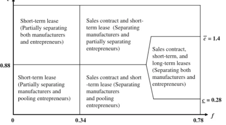
Assume the following values for the parameters employed in the basic model:d= 0.6,x= 16,cL= 5,
b= 1.05,h= 0.5, and/= 0.3. Based on these numbers, we depict inFig. 2the equilibrium characterized inProposition 2, as well as the equilibria characterized in the following sections. We depict these equi-libria incfspace: On thec-axis, we start from the situation where the difference in maintenance cost between the type H and type L entrepreneurscis small and end at the situation wherecis large; on thef-axis, we start from the situation where the quality factorfis small (i.e., difference in equip-ment quality between the two types of manufacturer is large) and end at the situation wherefis large and close to cL
ð1dÞx¼0:78, the maximum value offunder our assumption. Thus, we characterize the equilibria for the entire range of values ofc2(0,1) andf2 0; cL
ð1dÞx
. It is worth noting thatccan be viewed as measuring the extent of asymmetric information faced by the manufacturer regarding the entrepreneur. Whenc is larger, the extent of asymmetric information facing the manufacturer about the entrepreneur is larger. Similarly,fcan be viewed as measuring the extent of asymmetric information faced by the entrepreneur regarding the manufacturer. Whenfis smaller, the extent of asymmetric information facing the entrepreneur about the manufacturer is larger. Thus, we character-ize the equilibria for the entire range of situations where the manufacturer and the entrepreneur face various degrees of asymmetric information. It can be shown that the equilibrium that we characterize in each range of parameter values is unique. We now move on to briefly discuss the conditions under which these equilibria will differ from the one inProposition 2, i.e., we will characterize all the other equilibria presented inFig. 2.
f c 0.78 c= 0.28 c = 1.4 0.88 4 3 . 0 0 Sales contract, short-term, and long-term leases (Separating both manufacturers and entrepreneurs) Sales contract and short
-term lease (Separating manufacturers and pooling entrepreneurs) Sales contract and short-term lease (Separating manufacturers and partially separating entrepreneurs) Short-term lease (Partially separating both manufacturers and entrepreneurs) Short-term lease (Partially separating manufacturers and pooling entrepreneurs)
Fig. 2.Characterization of the entire range of equilibria with respect to the maintenance cost differentialcand the quality factorf.
4.2. Equilibria with only a short-term lease and a sales contract offered
When the difference in the maintenance costs between the type H and the L entrepreneur is larger than that characterized inProposition 2so that the maintenance cost of the type H is sufficiently large, the profit generated by the equipment if used by a type H entrepreneur during the second and the third periods will be smaller than the residual value of the equipment to the type G manufacturer. This will be the case whencH> (1d)x, so that the type H entrepreneur does not find it optimal to
main-tain the type G equipment. It could also happen when the type H has an incentive to mainmain-tain the type G equipment (i.e.,cH6(1d)x) but the cash flow generated by the type H entrepreneur net of the
maintenance cost is still sufficiently small. In both cases, the type G manufacturer has an incentive to repossess the equipment from the type H entrepreneur after the first period.24The following
prop-osition characterizes this situation.
Proposition 3 (Manufacturers separate and entrepreneurs partially separate: a short-term lease and a sales contract offered). When the quality factor is large enough (fPf) and the difference in the maintenance cost between the type H and L entrepreneur is large enough (cPc), then the equilibrium in the capital goods market involves the following:
(i) The type G manufacturer offers only a short-term leasing contract and the type B manufacturer offers only a sales contract.
(ii) If the manufacturer offers the short-term leasing contract, the type L entrepreneur accepts the con-tract, purchases the equipment at time 1, and performs maintenance in the first and the second per-iod; the type H entrepreneur accepts the contract as well, uses the equipment for one period without performing maintenance, and does not purchase the equipment at time 1. Both types of entrepreneur believe the manufacturer to be of type G with probability one in this case.
(iii) If the manufacturer offers only a sales contract, both the type H and type L entrepreneurs accept the sales contract and do not perform maintenance, believing the manufacturer to be of type B with probability one.
When the quality difference between the type G and type B equipment is the same as that in Prop-osition 2while the difference in the maintenance cost is larger than that inProposition 2, the type G manufacturer offers only a short-term lease and the type B manufacturer offers a sales contract in equilibrium. Following the same intuition as inProposition 2, the short-term lease in this equilibrium can help the type G manufacturer to achieve the separation from the type B manufacturer. Further, the short-term lease also enables the type G manufacturer to separate the type H entrepreneur from the type L entrepreneur and maximize his expected payoff. WhencPc, the type G manufacturer prefers to repossess his equipment from the type H entrepreneur after the first period while enabling the type L entrepreneur to utilize the equipment for as long a period as possible. To achieve this, the type G manufacturer sets the purchase price of his short-term lease high enough that the type H entrepreneur does not find it optimal to exercise the purchase option after the initial leasing period, while the type L entrepreneur will exercise it.25
In the above equilibrium, if the entrepreneur facing a type G manufacturer turns out to be of type L, the first best outcome would be achieved, since a type L entrepreneur will accept the short-term lease
24
Note that the type G manufacturer still prefers the type H entrepreneur to use the equipment for the first period, since the entrepreneur is able to generate more cash flows from new equipment compared to the manufacturer himself.
25
In this case, a long-term leasing contract (or a combination of a long-term and a short-term contract) is an inferior choice for the type G manufacturer compared to a short-term lease even if the long-term lease could also help the type G manufacturer separate himself from the type B manufacturer. First, given the high maintenance cost of the type H entrepreneur and the potential lack of maintenance, the type G manufacturer prefers to repossess his equipment from the type H entrepreneur after the first period. Second, the initial leasing price that can be charged by the type G manufacturer is constrained by the need to prevent mimicking from the type B manufacturer. This implies that the type G manufacturer would sacrifice more of his expected cash flow when he offers a leasing contract with a longer initial leasing period. As a result, a long-term lease will not be offered in equilibrium. In summary, the interaction between the asymmetric information existing on the manufacturer’s side and the asymmetric information existing on the entrepreneur’s side drives the equilibrium choice of contracts offered by the manufacturer in this setting.
and purchase the equipment at the end of the first period (performing maintenance in the first two periods). If, however, the entrepreneur facing the type G manufacturer turns out to be of type H, then clearly the first best outcome is not achievable for the type G equipment, and the appropriate bench-mark is the second best outcome. In this case, the second best outcome may or may not be achievable, depending on the maintenance cost of the type H entrepreneur.26The first best outcome is achieved for
the type B equipment here, since the first best outcome requires type B equipment to be used by either type of entrepreneur for all three periods without performing maintenance.
We now consider the case where the quality difference between the type G and type B equipment is the similar to that inProposition 2, but the difference in the maintenance costs between the type H and type L entrepreneur is smaller than that inProposition 2. The following proposition characterizes this situation.
Proposition 4 (Manufacturers separate and entrepreneurs pool: a short-term lease and a sales contract offered).When the quality factor is large enough that fPf while the difference in the maintenance cost between the type H and L entrepreneur is small enough that c<c, then the equilibrium in the capital goods market involves the following:
(i) The type G manufacturer offers a short-term leasing contract, and the type B manufacturer offers only a sales contract.
(ii) If the manufacturer offers the above leasing contract, both the type L and the type H entrepreneur accept the short-term contract, purchase the equipment at time 1, and perform maintenance in the first and the second period. Both types of entrepreneur believe the manufacturer to be of type G with probability one in this case.
(iii) If the manufacturer offers only a sales contract, both the type H and type L entrepreneurs accept the sales contract and do not perform maintenance, believing the manufacturer to be of type B with probability one.
As discussed underProposition 2, whether it is optimal for the type G manufacturer to have a type H entrepreneur use his equipment for two or three periods depends on the maintenance cost of the type H entrepreneur, the potential damage to the equipment due to lack of maintenance, and the reduction in the type G manufacturer’s profit from having to charge a lower price which would allow a type H entrepreneur to break even. Under the conditions characterized in this proposition, the type H entrepreneur’s maintenance cost is small enough that the type G manufacturer’s profit from the type H entrepreneur’s use of the equipment for an additional two periods exceeds his sacrifice in the profit that he would earn from charging a fair price to the type L entrepreneur. Consequently, the optimal choice for the type G manufacturer is to enable both the type L and type H entrepreneurs to use the equipment for all three periods. The type G manufacturer can achieve this by offering a short-term leasing contract, and charging a purchase price that is low enough that both the type H and the type L entrepreneur will exercise the purchase option at time 1. The short-term lease offered can also help the type G manufacturer to signal his firm type to the entrepreneur for the reasons dis-cussed in the previous propositions.27
26
If her maintenance cost is large enough thatProposition 1(i.c.) holds, i.e.cPxbd2xcL, then the second best is achievable, since in this case, the second best outcome calls for the type G equipment to be used by the type H entrepreneur for only one period, which is the case in this proposition. If, however, her maintenance cost is smaller, so that it is in the range where either
Proposition 1(i.a.) orProposition 1(i.b.) holds, i.e.,c<xbd2
xcL, then the second best is not achievable, since the second best outcome requires the type G equipment to be used for more than one period.
27
In the above equilibrium, if the entrepreneur facing a type G manufacturer turns out to be of type L, the first best outcome would be achieved, since a type L entrepreneur will accept the short-term lease and purchase the equipment at the end of the first period for another two periods (performing maintenance in the first two periods). If, however, the entrepreneur facing the type G manufacturer turns out to be of type H, then clearly the first best outcome is not achievable for the type G equipment, and the second best is the appropriate benchmark. In this case, the second best outcome will be achieved, since the second best outcome in this range of parameter values calls for the type G equipment to be used by the type H entrepreneur for all three periods with maintenance performed for the first two periods (seeProposition 1(i.a.)). The first best outcome is achieved for the type B equipment here, since the first best outcome requires type B equipment to be used by either type of entrepreneur for all three periods without performing maintenance.