Evaluating the Area of a Circle and the Volume of a Sphere by Using Monte Carlo Simulation
Abd Al - Kareem I. Sheet *
E.mail: [email protected]
ABSTRACT:
In this reseach Monte Carlo simulation is used to calculate the area of any circle as well as the volume of any sphere numerically. Different functions are considered to test the performance of this method, in addition to some improvement to give more satisfactory results. ﺓﺭﻜﻟﺍ ﻡﺠﺤﻭ ﺓﺭﺌﺍﺩﻟﺍ ﺔﺤﺎﺴﻤ ﺏﺎﺴﺤ ﻭﻟﺭﺎﻜ ﺕﻨﻭﻤﻟﺍ ﺓﺎﻜﺎﺤﻤ ﻡﺍﺩﺨﺘﺴﺎﺒ ﺹﺨﻠﻤﻟﺍ : ﺓﺭﺌﺍﺩ ﺔﻴﺃ ﺔﺤﺎﺴﻤ ﺏﺎﺴﺤﻟ ﻭﻟﺭﺎﻜ ﺕﻨﻭﻤﻟﺍ ﺓﺎﻜﺎﺤﻤ ﻡﺍﺩﺨﺘﺴﺍ ﻡﺘ ﺙﺤﺒﻟﺍ ﺍﺫﻫ ﻲﻓ ﺎﻴﺩﺩﻋ ﺓﺭﻜ ﺔﻴﺃ ﻡﺠﺤ ﺏﺎﺴﺤ ﻰﻟﺇ ﺔﻓﺎﻀﺇ . لﺍﻭﺩ ﺓﺩﻋ ﺏﺎﺴﺤ ﻡﺘ ﺔﻘﻴﺭﻁﻟﺍ ﻩﺫﻫ ﺀﺍﺩﺃ ﺭﺎﺒﺘﺨﻻﻭ ﺔﻔﻠﺘﺨﻤ ، ﻥﻋ ﻼﻀﻓ ﻟﺍ ﻩﺫﻫ ﻰﻠﻋ ﺕﺎﻨﻴﺴﺤﺘﻟﺍ ﺽﻌﺒ لﺎﺨﺩﺇ ﺭﺜﻜﺃ ﺔﻌﻨﻘﻤ ﺞﺌﺎﺘﻨ ﻲﻁﻌﺘﻟ ﺔﻘﻴﺭﻁ . 1- Introduction:
The evaluation of plane area, in particular the determination of the area of the circle, is one of the oldest problems in mathematics and seems to have been started in every culture where men have dealt with mathematical problems. The earliest attempts at measuring the area of a circle are thought to have been undertaken by the Babylonian and the Egyptian. The Babylonians discovered the fact that the radius of a circle is the side-length of an inscribed regular hexagon. The Egyptians discovered a good approximation of
*Univ. of Mosul - College of Basic Education - Dep .of Mathematics
the area of a unit circle which is equivalent to 3.1605. The next real progress came during the Greek period, Archimedes proved that the area between a second-order parabola and one of its tangents is a rational number (Engels, 1981).
This paper discusses Monte Carlo simulation, a classical yet unorthodox application of the method which is equivalent to making simulation of a function. The discussion is started briefly with the Monte Carlo simulation basics, then explaining the use of this technique to solve two theoretical problems :
1- The estimation of the area of a circle through random sampling.
2- A generalization of this idea to calculate the estimation of the volume of a sphere.
In order to increase the accuracy of the method used in sampling in this paper, the average of the results of 10 runs for each value of the sample size n are taken.
2- Basic Monte Carlo Simulation:
A Monte Carlo simulation is a generic numerical method using a computer utilizing pseudo-random numbers to simulate stochastic inputs to a process and generate large numbers of possible outcomes. It solves a problem by generating suitable random numbers and observing that fraction of the numbers obeying some property or properties (Sabelfeld, 2004). It is commonly used for simulations in many fields that require solutions for problems that are impractical or impossible to solve by traditional analytical or numerical methods (Yang, 2002). The Monte Carlo simulation is mainly used to predict the final consequence of a series of occurrences, each having its own probability. A major requirement in Monte Carlo simulation is that the mathematical system be described by probability density functions. Once the density functions are known, the Monte Carlo simulation can proceed by random sampling from these density functions for use within the simulation. Given that a particular simulation outcome is based randomness performing the same simulation again would, most
likely result is a different outcome. Many simulations are performed and the desired result is taken as an average over the number of outcomes (Smaldone, 2001).
The main steps of Monte Carlo Simulation are (Stokes, 2004): 1) Model the inputs and process.
2) Draw a vector of random varieties. 3) Evaluate the function of interest.
4) Repeat the last two steps many times, aggregating the results.
3- Simulating Deterministic Behavior:
In this section we illustrate the use of Monte Carlo simulation to model a deterministic behavior, the area of a circle and the volume of a sphere, were Monte Carlo technique can be extended to functions of several variables and become more practical in that situation.
3.1- Simulating the Area of a Circle:
We want to construct a simulation which will estimate the area of a circle. A program is written to play with Monte Carlo methods, it uses the relationship between
π
and the area of a circle,2
r
A= π . An elegant way to visualite the relationship is to imagine
slicing a circle into smaller pieces, then rearranging these pieces into a rectangle. The area of the rectangle is equal to the area of the circle and is equal to its radius r multiplied by its length
π
r
, or2
r
A= π .
The trick with Monte Carlo simulation is to find a function that includes your unknown function of interest, then guess values and evaluate if they are included in your function of interest. The fraction that is contained is proportional to the fraction of the area of the unknown function in your known function area.
The discussion of Monte Carlo simulation to model a deterministic behavior ( the area of a circle), is as follows: Consider the following general case equation of the circle
2 2
2 ( )
)
In order to estimate the area of this circle through random sampling, the following algorithm is suggested.
Monte Carlo area algorithm:
Input: The radius r, the center (a,b), and the total number n of
random points to be generated during the simulation.
Output: Area of the circle.
Step 1: Generate n uniform random sequences
xi∈[a−r,a+r] (2)
Step 2: Calculate the simulation function ( ) 2 2 ( )2
a x r x
f i = − i −
which correspons to the equation (1) for the random xi coordinates.
Step 3: Calculate
∑
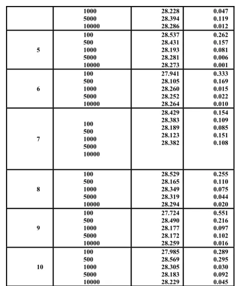
= = n i i n r f x circle the of Area 1 2 ( ) (3) Step 4: Stop.Table (1) summarizes the results of 10 different simulations to obtain the estimation of the area of a circle defined by the equation: ( − 3)2 + ( − 2)2 = 9
y
x (4)
using drand48 (seed = 1) as a random number generators. Approximations were made using n = 100, 500, 1000, 5000, and 10000 terms in the summation, each approximation was compared to the exact value of the area ( = 28.274 2
cm ).
Table.1: Monte Carlo approximation to the area of a circle, drand48.
Run Number Length of simulation run Estimated Area Absolute Error 1 100 500 1000 5000 10000 28.132 28.110 28.347 28.156 28.256 0.142 0.164 0.073 0.118 0.018 2 100 500 1000 5000 10000 28.629 28.312 28.159 28.356 28.251 0.354 0.038 0.116 0.081 0.023 3 100 500 1000 5000 10000 27.823 28.237 28.239 28.313 28.331 0.451 0.037 0.035 0.039 0.056 4 100 500 28.39728.125 0.122 0.149
1000 5000 10000 28.228 28.394 28.286 0.047 0.119 0.012 5 100 500 1000 5000 10000 28.537 28.431 28.193 28.281 28.273 0.262 0.157 0.081 0.006 0.001 6 100 500 1000 5000 10000 27.941 28.105 28.260 28.252 28.264 0.333 0.169 0.015 0.022 0.010 7 100 500 1000 5000 10000 28.429 28.383 28.189 28.123 28.382 0.154 0.109 0.085 0.151 0.108 8 100 500 1000 5000 10000 28.529 28.165 28.349 28.319 28.294 0.255 0.110 0.075 0.044 0.020 9 100 500 1000 5000 10000 27.724 28.490 28.177 28.172 28.259 0.551 0.216 0.097 0.102 0.016 10 100 500 1000 5000 10000 27.985 28.569 28.305 28.183 28.229 0.289 0.295 0.030 0.092 0.045
From table (1) we observe the following:
1) The estimates of the area approach the exact value (= 28.274 cm2) as the number of points generated (or length of the simulation run) increases.
2) The 10 simulation runs do yield different estimates given the same n. Each run actually may be regarded as an observation
in the simulation experiment.
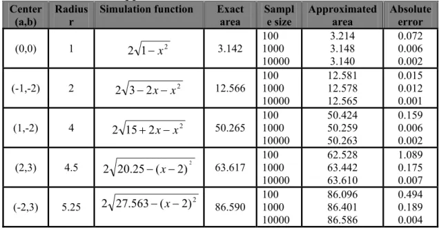
Table 2 illustrates our results for various choices of centers (a, b), radiuses r. Approximations were made using n = 100, 1000, and
10000 terms in the summation, each approximation was compared to the exact value of the area.
Table 2: Monte Carlo approximation to the area of 5 circles; rand.
Center
(a,b) Radius r Simulation function Exact area Sample size Approximated area Absolute error
(0,0) 1 2 1 2 x − 3.142 100 1000 10000 3.214 3.148 3.140 0.072 0.006 0.002 (-1,-2) 2 2 3 2 2 x x− − 12.566 100 1000 10000 12.581 12.578 12.565 0.015 0.012 0.001 (1,-2) 4 2 15 2 2 x x− + 50.265 100 1000 10000 50.424 50.259 50.263 0.159 0.006 0.002 (2,3) 4.5 2 ) 2 ( 25 . 20 2 − x− 63.617 100 1000 10000 62.528 63.442 63.610 1.089 0.175 0.007 (-2,3) 5.25 2 27.563−(x−2)2 86.590 100 1000 10000 86.096 86.401 86.586 0.494 0.189 0.004
From table 2 we observe that the estimates of the area of each circle approach to the exact value of the area as the number of points generated increases.
Figure 1-a plots the estimated area of the circle defined by equation (4) for run 1 (blue curve) and run 2 (red curve) given in table 1 and the exact value (= 28.274 cm2 green curve) against the length of the simulation run n.
Figure 1-a: Approximated area for run 1 and 2.
From figure 1-a we can see that initially, the estimates oscillate around the exact value before eventually stabilizing a condition normally reached after the simulation experiment is repeated a sufficiently large number of times.
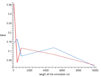
Figure 1-b plots the absolute error given in table 1 for runs 1 (blue curve) and 2 (red curve) against the length of the simulation run n.
From figure 1-b we observe that initially, the absolute error decreases as the number of points generated increase.
3.2- Estimation of the Volume of a Sphere by Simulation:
Let's consider finding part of the volume of the sphere x2 +
y2 + z2 ≤ 1 that lies in the first octant ; x > 0, y > 0, z > 0. The methodology to approximate the volume is very similar to that of finding the area under a closed curve, however, now we will use an approximation for the volume under the surface by the following rule: s po of number total t oc st in surface below counted s po of number box of volume surface under volume int tan 1 int ≅
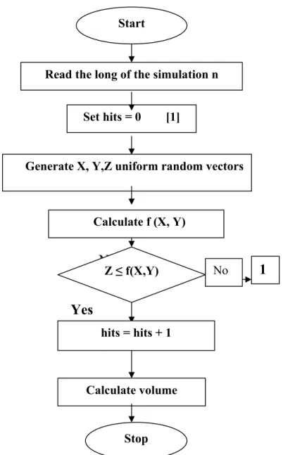
Figure (2) shows the sequence of calculations required to employ Monte Carlo techniques to find approximate volume under a surface.
No
Yes
Figure 2: Flow chart for Monte Carlo simulation volume algorithm. Table 3 summarizes the results of several different simulations to obtain the estimation of the volume of the sphere x2 + y2 + z2 ≤ 1 using rand as a random number generator. Approximations were made using n =100, 500, 1000, 5000 and
10000 terms in the summation, each approximation was compared to the exact value of the volume (=4.189 cm3 ).
Start
Set hits = 0 [1]
Generate X, Y,Z uniform random vectors
Calculate f (X, Y) Read the long of the simulation n
Z ≤ f(X,Y) 1
Calculate volume
Stop hits = hits + 1
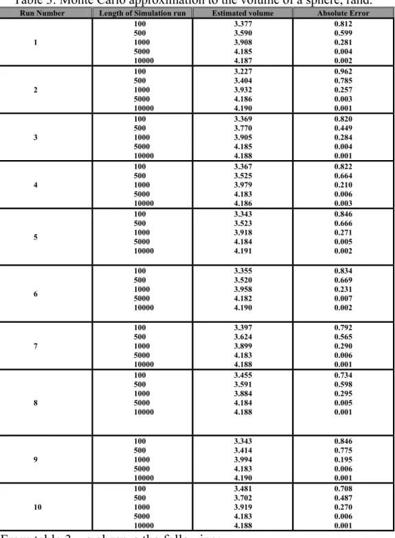
Table 3: Monte Carlo approximation to the volume of a sphere, rand.
Run Number Length of Simulation run Estimated volume Absolute Error
1 100 500 1000 5000 10000 3.377 3.590 3.908 4.185 4.187 0.812 0.599 0.281 0.004 0.002 2 100 500 1000 5000 10000 3.227 3.404 3.932 4.186 4.190 0.962 0.785 0.257 0.003 0.001 3 100 500 1000 5000 10000 3.369 3.770 3.905 4.185 4.188 0.820 0.449 0.284 0.004 0.001 4 100 500 1000 5000 10000 3.367 3.525 3.979 4.183 4.186 0.822 0.664 0.210 0.006 0.003 5 100 500 1000 5000 10000 3.343 3.523 3.918 4.184 4.191 0.846 0.666 0.271 0.005 0.002 6 100 500 1000 5000 10000 3.355 3.520 3.958 4.182 4.190 0.834 0.669 0.231 0.007 0.002 7 100 500 1000 5000 10000 3.397 3.624 3.899 4.183 4.188 0.792 0.565 0.290 0.006 0.001 8 100 500 1000 5000 10000 3.455 3.591 3.884 4.184 4.188 0.734 0.598 0.295 0.005 0.001 9 100 500 1000 5000 10000 3.343 3.414 3.994 4.183 4.190 0.846 0.775 0.195 0.006 0.001 10 100 500 1000 5000 10000 3.481 3.702 3.919 4.183 4.188 0.708 0.487 0.270 0.006 0.001
1. The estimates of the volume approach the exact value (= 4.189 cm3) as the number of points generated increases.
2. The 10 simulation runs do yield different estimates given the same n. Each run actually may be regarded as an observation
in the simulation experiment.
Figure 3-a plots the volume estimates for runs 1 (blue curve) and 2 (red curve) and the exact value (= 4.189 cm3 green curve) against the length of the simulation run n.
Figure 3-a: Approximated volume for run 1 and2.
From figure 3-a we see that initially, the estimates increase reaching the exact value as the number of points generated increases.
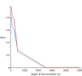
Figure 3-b plots the absolute error given in table 3 for run 1 (blue curve) and 2 (red curve) against the length of the simulation run n.
Figure 3-b: Volume absolute error for run 1 and 2. From figure 3-b we observe that initially, the absolute error decreases as the number of points generated increase.
4- Improved Monte Carlo Simulation:
A straightforward method for speeding up the Monte Carlo simulation algorithm is to use a large sample size and a long simulation run. One of the most important methods to speed the convergence of the Monte Carlo area and volume algorithm discussed in section 3.1 and 3.2 is to average the results of the simulation runs. Table 4 summarizes the mean and the absolute error of the results given in table (1) of the 10 runs for each n = 100,
500, 1000, 5000, and 10000.
Table 4: Average results of the 10 runs.
n 100 500 1000 5000 10000
Mean 28.123 28.293 28.245 28.255 28.286
Abs error
0.151 0.019 0.029 0.019 0.012
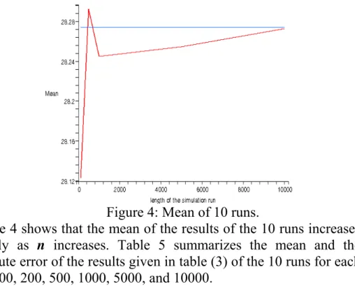
From table 4 we observe that it is interesting that the effect of transient conditions is dampened when we average the results of the 10 runs. This result can be seen clearly in figure 4, where we plot
the mean (red curve), and the exact value (=28.274 cm2 blue curve) against the length of the simulation run n.
Figure 4: Mean of 10 runs.
Figure 4 shows that the mean of the results of the 10 runs increases rapidly as n increases. Table 5 summarizes the mean and the
absolute error of the results given in table (3) of the 10 runs for each
n = 100, 200, 500, 1000, 5000, and 10000.
Table 5: Average results of the 10 runs.
n 100 200 500 1000 5000 10000
Mean 3.371 3.434 3.566 3.930 4.184 4.189
Abs
error 0.818 0.755 0.623 0.256 0.005 0.000
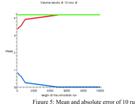
From table 5 we observe that it is interesting that the effect of transient conditions is dampened when we average the results of the 10 runs. This result can be seen clearly in figure 5, where we plot the mean (red curve), the absolute error (blue curve), and the exact value (=4.189 cm3 green curve) against the length of the simulation run n.
Figure 5: Mean and absolute error of 10 runs. Figure 5 shows that the mean of the results of the 10 runs increases rapidly as the length of the simulation run n increases, while the
absolute error decreases rapidly as n increases. 5- Discussion:
The present work deals with Monte Carlo simulation problem. Two methods are presented to calculate the area of a circle and the volume of a sphere. Many programs are prepared according to the above mentioned methods and their application on a set of corresponding functions for the general formula of circle equation and the equation of a sphere centered at the origin with unit radius. The suggested Monte Carlo simulation algorithms was accelerated by using two techniques, the first is the increase of sample size used, the second which is more important is to find the average of simulation results. The work concluded that these two techniques are necessary for speeding up the rate of convergence of Monte Carlo simulation algorithms used to calculate the area of a circle and the volume of a sphere, and finally to get more accurate estimators with less possible absolute error.
References:
1- Engels, H. (1980)," Numerical Quadrature and Cubature ", Academic Press, New York.
2- Stokes, V. P. (2004), " Monte Carlo simulation: basics ", Survey Report, Uppsala Univ. Press.
3- Sabelfeld, K. K. (2004), " Monte Carlo methods and applications ", Monte Carlo Methods, Vol. 10.
4- Smaldone, Tony, 2001, " Modeling and Simulation ", Mc- Graw Hill, New York.
5- Yang, Guan, 2002," A Monte Carlo Method of Integration ", The Chemical Rubber Company Press.