Finding Fastest Paths on A Road Network with Speed Patterns
Evangelos Kanoulas
Yang Du
Tian Xia
Donghui Zhang
∗College of Computer & Information Science Northeastern University, Boston, MA 02115
{ekanou, duy, tianxia, donghui}@ccs.neu.edu
Abstract
This paper proposes and solves the Time-Interval All Fastest Path (allFP) query. Given a user-defined leaving or arrival time intervalI, a source nodesand an end nodee, allFP asks for a set of all fastest paths fromstoe, one for each sub-interval ofI. Note that the query algorithm should find a partitioning ofI into sub-intervals. Existing methods can only be used to solve a very special case of the problem, when the leaving time is a single time instant. A straightfor-ward solution to the allFP query is to run existing methods many times, once for every time instant in I. This paper proposes a solution based on novel extensions to the A* al-gorithm. Instead of expanding the network many times, we expand once. The travel time on a path is kept as a function of leaving time. Methods to combine travel-time functions are provided to expand a path. A novel lower-bound estima-tor for travel time is proposed. Performance results reveal that our method is more efficient and more accurate than the discrete-time approach.
1
Introduction
Have you ever been stuck in traffic while driving, wish-ing that you had known a better route? In the United states, only 9.3% of the households do not have cars. Driving is part of people’s daily life. GIS systems like MapQuest and MapPoint are heavily relied on to provide driving di-rections. However, surprisingly enough, existing systems either ignore the driving speed on road networks, or as-sume the speed remains constant on the road segments. In both cases the users’ preferred leaving time does not af-fect the query result. For instance, MapQuest does not ask the users to input the day and time of driving. But we all know that during rush hours, inbound highways to big cities have much lower speed than usual. So a fastest path com-puted during non-rush hours, which may consists of some
∗Partially supported by NSF CAREER Award IIS-0347600.
inbound highway segments, may not remain the fastest path during rush hours.
To capture speed changes, we propose the CAtegorized PiecewisE COnstant speeD (CapeCod) pattern, which is an extension of the Flow Speed Model (FSM) [19] by in-corporating categorized speed patterns. Here days are cat-egorized, e.g. workdays and non-workdays. Within each category, we assume the speed on each road segment is piecewise constant. For instance, in a working day, dur-ing rush hour (say from 7am to 9am) the speed is 0.3 miles per minute (mpm), and at other times of the day the speed is 1mpm.
The paper proposes and solves the Time Interval All Fastest Paths (allFP) Query, on a road network with CapeCod speed patterns. As the road network may be large, it is reasonable to assume that it is stored on disk. We adapt the Connectivity-Cluster Access Method (CCAM) [18] to store and access the network information. Besides the source nodesand the end nodee, a query consists of a leaving time interval at s (or e). All fastest paths are enumerated, each corresponding to a disjoint sub-interval of leaving time. The union of all sub-intervals should cover the entire query time interval. An allFP query example is: I may leave for work any time between 7am and 9am; please suggest all fastest paths, e.g. take route A if the leaving time is between 7 and 7:45, and take route B otherwise.
A variation is the Time Interval Single Fastest Path (sin-gleFP) query, which only reports a single fastest path: the one that minimizes the travel time among all leaving time instants in the query time interval.
If instead of a time interval, a single leaving time instant is given, both allFP and singleFP correspond to the same special case, which is trivial. The special case actually de-grades into the shortest-path problem. The reason is that for each edgeni → nj, if we know the leaving time instant
at ni, the arrival time atnj is fixed. This special case is
a well studied problem in multiple disciplines: transporta-tion systems, networks, graph theory, artificial intelligence, and spatial databases. One of the best algorithms, named A* [15], extends Dijkstra’s single-source-shortest-path
al-gorithm. The idea is as follows. Keep a setEof expanded nodes (initially empty) and a priority queue F of frontier nodes (initially consisting only of the source nodes). Each iteration chooses one node fromF, expands it by adding its non-expanded neighbors toF, and moves it toE. To choose the next node fromF, instead of choosingiwhere the travel time fromstoiis the smallest (as in Dijkstra’s algorithm), choose the nodejsuch that the travel time fromstojplus the estimated travel time from j toeis the smallest. As pointed in[15], the estimation must be a lower bound of the actual travel time to ensure correctness. Also, the closer the estimation is to the actual travel time, the more efficient the search is.
In allFP and singleFP queries, the leaving timelatsis not fixed, but can be any instant in a given intervalI. In this case, the travel time on each road segment is a function of time and therefore, none of the existing algorithms can be applied to solve these queries. For instance, in A*, in each iteration a node is chosen to be expanded. In the new queries, since different leaving time suggests that different nodes should be expanded, which one do we choose? To get around this problem, one approach to answer the new queries (but only approximately) is to assume discrete time model. For instance, if we assume the leaving time can only be at the very beginning of every minute, we can call the A* algorithm many times, one per minute. But this approach is neither accurate nor efficient.
We propose an algorithm called IntAllFastestPaths to ac-curately and efficiently solve the allFP query. One interme-diate step of the algorithm identifies the result for the sin-gleFP query, and therefore the algorithm also can answer the singleFP query, without spending the time to find the complete result for the allFP query. The algorithm consists of some novel extensions to the A* Algorithm. (i) Each en-try in the priority queue has a travel-time function instead of a single travel time value, and we tell which node should be expanded in each iteration. (ii) Given the travel-time func-tionT1(l ∈I)of a paths ⇒ni and an edgeni →nj, we
discuss how to determine the intervalI0of leaving time at
ni. (iii) Once we get such an interval and the
correspond-ing functionT2(l0 ∈I0), we present a way to combineT1()
withT2()to get the new travel function for the expanded
paths ⇒ ni → nj. (iv) Another important issue is how
to provide a lower-bound estimation to the travel time from some nodenj to the end nodee. A straightforward choice
is to use the Euclidean distance divided by the maximum speed in the network, as it is guaranteed to be a lower bound of the actual travel time. In Section 5, we propose a better (i.e. closer to the actual travel time) estimator, namely the boundary node estimator.
The major contributions of the paper are:
1. We propose the allFP query and its variation the sin-gleFP query, where the speed changes are captured by
the CapeCod patterns. By allowing the users to pro-vide a leaving time interval, the queries are practical extensions to the queries considered in existing path-computation systems.
2. We present an algorithm (IntAllFastestPaths) to solve the two fastest-path queries. The algorithm is based on novel extensions to A*. The priority queue stores travel-time functions associated with expanded paths. We describe how to choose a path to keep expanding, how to determine the leaving time interval at each in-termediate node, and how to produce the compounded function for the newly expanded path (Section 4). 3. We provide a novel lower-bound estimator to reduce
the search space (Section 5). The estimator is based on graph partitioning and pre-computation.
The rest of the paper is organized as follows. Problem definition appears in Section 2. Related work is reviewed in Section 3. The fastest-path algorithms are presented in Section 4. The new lower-bound estimator appear in Sec-tion 5. Performance results are shown in SecSec-tion 6. Finally, Section 7 concludes the paper.
2
Problem Definition
This section formally defines the CapeCod patterns, the road network which incorporates these patterns and the two queries addressed in this paper. The storage model and the required operations are also discussed.
2.1
CapeCod Network and Fastest Path Queries
Definition 1 A (day-)category setD is a list of categories such that each day belongs to exactly one category in D. For any two days belonging to the same category, a road segment exhibits the same speed patterns.
For example, such a category set may be: workday, non-workday. Here the assumption is that for two days in the same category, a road segment has the same speed at the same time of day. Although this may not be 100% accu-rate, it is a reasonable assumption for two reasons. First, if the volume of traffic on a road segment is high at some time on one workday, it is likely the same to happen the same time on another workday. Second, the approximation becomes more accurate by increasing the number of cate-gories. For instance, if for some road segment the speed pattern for Fridays is different from that of other workdays, we can identify Friday as another category.
Definition 2 Given a category setD, a CAtegorized Piece-wisE COnstant speeD (CapeCod) pattern consists of one
daily speed pattern for every day-category inD. Here each daily pattern has piecewise constant speed for the 24-hour duration.
An example of a CapeCod pattern may be: for a non-workday: [0:00-24:00):1mpm1; and for a workday: [0:00-7:00):1mpm, [7:00-9:00):1/2mpm, [9:00-24:00):1mpm. This pattern indicates that traffic congestion occurs every workday from 7am to 9am.
Definition 3 Given a category set D, a CapeCod net-work is a directed graph G(N, E) such that, N = {(ni, loci)|i ∈ [1, m]} is the set of nodes (road
inter-sections and end points) with their spatial locations, and E ={(ni, nj, dij, patij)|i, j ∈ [1, m]}is the set of edges
ni → nj, where dij is the distance and patij is the
CapeCod pattern.
The Flow Speed Model (FSM) in which the speed on each network edge is a piecewise-constant function, was proposed in [19]. The CapeCod model slightly extends FSM by involving a category of days to fit the need for spa-tial road networks.
Definition 4 Given a CapeCod network, a start node s and an end nodee, and a leaving time interval I, the All
Fastest Path (allFP) query returns a full partitioning of
I: I1, . . . , Ik, where each sub-interval is associated with
a fastest path, such that two leaving time instants in one sub-interval leads to the same fastest-path and two leaving time instants in two adjacent sub-intervals leads to different fastest paths.
While focusing on the allFP query, this paper also ad-dresses the single fastest path (singleFP) query. That is, given a start nodes, an end nodee, and a leaving time in-tervalI, find the time instantl0∈I and the corresponding
fastest path fromstoesuch that leaving fromsat timel0
minimizes the travel time fromstoe.
Both queries compute fastest paths from nodestoefor a leaving time intervalI. The singleFP query reports the best leaving time instant duringI to minimize travel time and the corresponding fastest path. The allFP query finds all different fastest paths, one per disjoint sub-interval ofI.
2.2
Storage Model
Assuming that the network has reasonably large size, it needs to be stored on disk. We adopt the connectivity-cluster access method (CCAM) [18] to store and access the network information.
1Here we use mile per minute instead of mile per hour to be consistent
with the examples in later sections.
In particular, for each nodeni, the corresponding
infor-mation to be stored on disk, denoted as inf oi, stores the
locationlociof it in space plus a list of neighbors. For each
neighbor,nj, we store its Euclidean distancedij from ni
and the CapeCod speed pattern of the road segmentpatij.
To cluster the information of nodes in disk pages, accord-ing to [18], we should preserve the connectivity relation-ship by heuristically partitioning the graph. Information for nodes in the same partition is stored in the same disk page.
On top of the disk pages that store the node information, a B+-tree is kept to efficiently locate the information of any node. The one-dimensional ordering of all nodes is gen-erated using the Hilbert values of their locations. CCAM supports all the necessary operations for our algorithms -such as F indN ode(ni)andGetSuccessor(ni)- and the
appropriate operations to update the network.
3
Related Work
Most existing work on path computation has been fo-cused on the shortest-path problem. Several extensions of the Dijkstra algorithm have been proposed, mainly focus-ing on the maintenance of the priority queue. The A* algo-rithm [15, 10] finds a path from a given start node to a given end node by employing a heuristic estimate. Each node is ranked by an estimate of the best route that goes through that node. A* visits the nodes in order of this heuristic es-timate. A survey on shortest-path computation appeared in [14].
Performance analysis and experimental results regard-ing the secondary-memory adaptation of shortest path algo-rithms can be found in [5, 17]. The work in [4] contributes on finding the shortest path that satisfies some spatial con-straints. A graph index that can be used to prune the search space was proposed in [20].
One promising idea to deal with large-scale networks is to partition a network into fragments. The boundary nodes, which are nodes having direct links to other fragments, con-struct the nodes of a high-level, smaller graph. This idea of hierarchical path-finding has been explored in the context of computer networks [9] and in the context of transportation systems [8, 6, 7]. In [16], the materialization trade-off in hierarchical shortest path algorithms is examined.
The fastest-path problem is a generalization of the shortest-path problem in the sense that the cost measure (in particular, the travel time) to traverse a road segments varies over time. This makes the fastest-path problem more com-plicated since the fastest path from a source nodesand an end nodeeis not unique and depends on the leaving time froms. One way to deal with this complexity is to assume a discrete-time model [1, 11]. [1] proposes a backward la-belling algorithm based on the assumption that the cost to traverse an edge remains constant after some time. [11]
ap-plies the A* algorithm for every leaving time instant simul-taneously. Discrete-time models effectively capture trans-portation networks (e.g. railway or bus networks) in which vehicles depart on particular time instants. However, re-garding road networks they are not accurate enough, since what happens between two adjacent time instants cannot be told. Moreover, discrete-time algorithms are not efficient. Suppose we want to know all fastest paths during some time interval (allFP Query). Independent to the number of differ-ent fastest paths (which may be small) in the answer set, the discrete-time algorithm needs to perform one query per time instant in the query interval. Even if this is done simultane-ously for all leaving time instants it is still computationally inefficient.
Another work on fastest-path computation is [12, 13]. However, the network model proposed is beyond GIS. For instance, it allows unrestricted waiting of objects at the nodes, which is not applicable in road networks since un-restricted waiting at road junctions is prohibited. Also, they consider the possibility of non-FIFO behavior, where an ob-ject that leaves a node later than a previous obob-ject may arrive the next-hop node earlier. Moreover, continuous-time mod-els necessitate the processing of functions of leaving time. Here, [12] only suggested operations on functions that are necessary without investigating how this operations can be supported. Therefore, regarding path computations in road networks, this work is of theoretical interest only.
The Flow Speed Model (FSM) has been proposed in [19]. In FSM the travel time on each road segmentni→nj
is a piece-wise linear function of the leaving time fromni.
The model is proven to preserve the FIFO property. The paper only addresses the fastest path query for a given leav-ing time instant. As we have discussed before, this makes the fastest path problem degrade to the shortest path prob-lem and therefore it avoids the complexity of manipulating continuous-time functions.
Moreover, [3] proposes a storage model and an update process of the speed on each road segment of road network. The network model used is discrete-time model. To solve the fastest path problem, the paper adopts an algorithm first proposed in [14] . Although the system proposed is highly adaptive to any change in the status of the road network it does not guarantee that the actual fastest path is found.
4
Fastest-Path Computation
In this section, we present the basic version of our algo-rithm. It novelly extends the A* algorithm, while using the Euclidean distance divided by maximum network speed as the lower-bound travel-time estimator.
4.1
From Speed Patterns To Travel Time
Func-tions
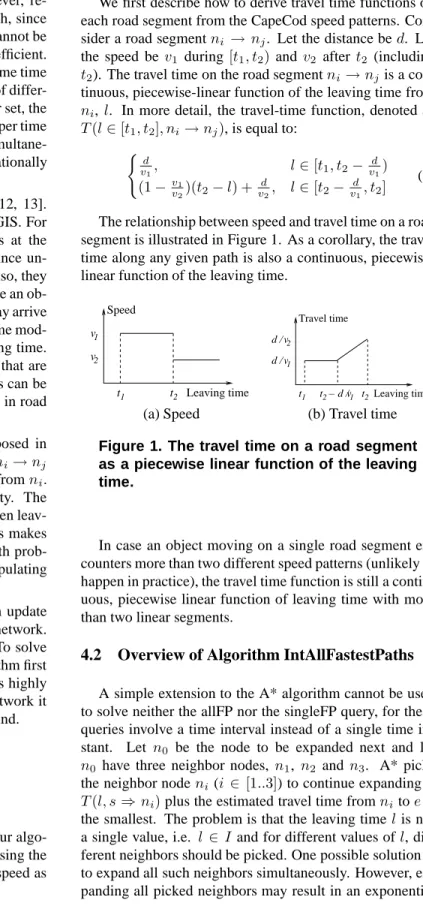
We first describe how to derive travel time functions on each road segment from the CapeCod speed patterns. Con-sider a road segmentni → nj. Let the distance bed. Let
the speed be v1 during[t1, t2)andv2 aftert2 (including
t2). The travel time on the road segmentni→nj is a
con-tinuous, piecewise-linear function of the leaving time from ni, l. In more detail, the travel-time function, denoted as
T(l∈[t1, t2], ni→nj), is equal to: (d v1, l∈[t1, t2−vd 1) (1−v1 v2)(t2−l) + d v2, l∈[t2− d v1, t2] (1)
The relationship between speed and travel time on a road segment is illustrated in Figure 1. As a corollary, the travel time along any given path is also a continuous, piecewise-linear function of the leaving time.
t1 v1 v2 t2 Speed Leaving time v1 v2 t1 t − d /2 v1 t2 Travel time d / d / Leaving time
(a) Speed (b) Travel time
Figure 1. The travel time on a road segment as a piecewise linear function of the leaving time.
In case an object moving on a single road segment en-counters more than two different speed patterns (unlikely to happen in practice), the travel time function is still a contin-uous, piecewise linear function of leaving time with more than two linear segments.
4.2
Overview of Algorithm IntAllFastestPaths
A simple extension to the A* algorithm cannot be used to solve neither the allFP nor the singleFP query, for these queries involve a time interval instead of a single time in-stant. Let n0 be the node to be expanded next and let
n0 have three neighbor nodes,n1, n2 andn3. A* picks
the neighbor nodeni(i ∈ [1..3]) to continue expanding if
T(l, s⇒ni)plus the estimated travel time fromni toeis
the smallest. The problem is that the leaving timel is not a single value, i.e. l ∈ I and for different values ofl, dif-ferent neighbors should be picked. One possible solution is to expand all such neighbors simultaneously. However, ex-panding all picked neighbors may result in an exponential
number of paths being expanded regardless the size of the answer set.
Instead, we propose a new algorithm called
IntAll-FastestPaths. The main idea of the algorithms is
summa-rized below:
1. Maintain a priority queue of expanded paths, each of which starts withs. For each paths ⇒ ni, maintain
T(l, s ⇒ ni) +Test(ni ⇒ e)as a piecewise-linear
function of l ∈ I. Here, Test(ni ⇒ e)is a lower
bound estimation function of the travel time fromni
to the end nodee. In the basic version, we choose the naive estimator,deuc(ni, e)/vmax, which is the
Eu-clidean distance betweenniande, divided by the max
speed in the network.
2. Similar to the A* Algorithm, in each iteration pick a path from the priority queue to expand. Pick the path, whose maintained function’s minimum value duringI is the minimum among all paths. Here, how to expand a path is non-trivial and will be discussed in details later in this section.
3. The first path ending toethat is picked from the pri-ority queue is the answer to the singleFP query. The optimal leaving time is the time instant at which the travel time function of the path is getting its minimum value.
4. Maintain a special travel-time function called the lower border function. It is the lower border of travel time functions for all identified paths (i.e. paths al-ready picked from the priority queue) that end toe. In other words, for any time instantl ∈I, the lower bor-der function has a value equal to the minimum value of all travel time functions of identified paths froms to e. This function consists of multiple travel time functions, each corresponding to some path fromsto eand some subinterval ofI during which this path is the fastest.
5. Stop either when there is no more path left in the pri-ority queue, or if the path picked to be expand next has a minimum value no less than the maximum value of the lower border function. Report the lower border function as the answer to the allFP query.
Below we use a running example to further describe the ideas of the algorithm.
4.3
Initialization
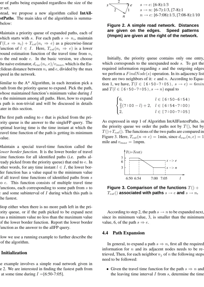
The example involves a simple road network given in Figure 2. We are interested in finding the fastest path from stoeat some time duringI =[6:50-7:05].
1 s e n 2 2 s→e: [6-8):1/3 s→n: [6-7):1/3, [7-8):1 n→e: [6-7:08):1/3, [7:08-8):1/10
Figure 2. A simple road network. Distances
are given on the edges. Speed patterns
(#mpm) are given at the right of the network.
Initially, the priority queue contains only one entry, which corresponds to the unexpanded node s. To get the required information regarding s and the outgoing edges we perform aF indN ode(s)operation. In its adjacency list there are two neighbors of it:eandn. According to Equa-tion 1, we have,T(l ∈[6:50-7:05), s→e) = 6min
andT(l∈[6:50-7:05), s→n)equal to 6, l∈[6:50-6:54) 2 3(7:00−l) + 2, l∈[6:54-7:00) 2, l∈[7:00-7:05]
As expressed in step 1 of Algorithm IntAllFastestPaths, in the priority queue we order the paths not by T(), but by T()+Test(). The functions of the two paths are compared in
Figure 3. Here,Test(n⇒e) = 1min, sincedeuc(n, e) = 1
mile andvmax= 1mpm.
T()+Test() 6:50 6:54 7:00 7:05 l 3 6 7 s −> n s −> e
Figure 3. Comparison of the functions T() +
Test()associated with pathss→eands→n.
According to step 2, the paths→nto be expanded next, since its minimum value, 3, is smaller than the minimum value, 6, of the paths⇒e.
4.4
Path Expansion
In general, to expand a paths⇒n, first all the required information for n and its adjacent nodes needs to be re-trieved, Then, for each neighbornjofnthe following steps
need to be followed:
• Given the travel time function for the paths⇒nand the leaving time intervalI froms, determine the time
interval during which the travel time function for the road segmentn→njis needed.
• Determine the time instantst1, t2, . . . ∈ I at which
the resulting function, i.e. the travel time function for the paths⇒nj,T(l∈I, s⇒nj), changes from one
linear function to another.
• For each time interval[t1, t2), . . ., determine the
cor-responding linear function of the resulting function T(l∈I, s⇒nj).
In our example, the time interval forn→eis determined to be [6:56, 7:07] as shown in Figure 4. At time 6:50 (start ofI), the travel time along the path s → n is 6 minutes. Therefore, the start of the leaving time interval forn → e, i.e. the start of arrival time interval to n, is 6:50+6min = 6:56. Similarly, the end of the leaving time interval is 7:05+2min = 7:07. T(l, s −> n) 6:50 6:54 6:56 7:00 7:05 l 6 7:07 2
Figure 4. The time interval, [6:56-7:07], during
which the speed onn→eis needed.
During the time interval [6:56-7:07], the travel time on
n→e,T(l∈[6:56-7:07], n→e)is
(
3, ifl∈[6:56-7:05)
10−7
3(7:08−l), ifl∈[7:05-7:07]
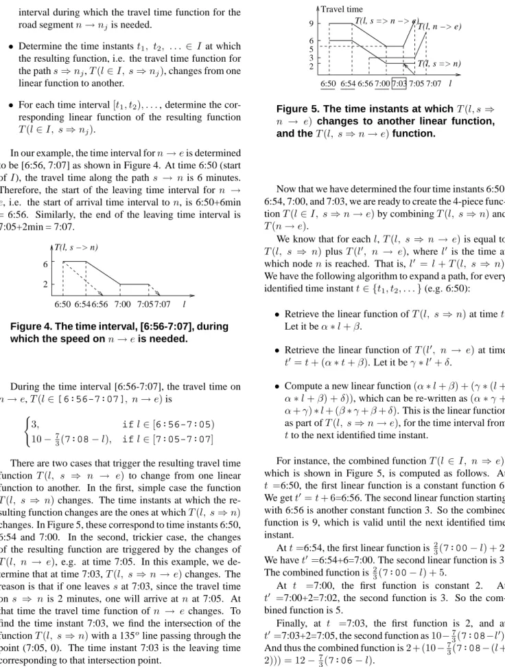
There are two cases that trigger the resulting travel time function T(l, s ⇒ n → e) to change from one linear function to another. In the first, simple case the function T(l, s ⇒ n)changes. The time instants at which the re-sulting function changes are the ones at whichT(l, s⇒n) changes. In Figure 5, these correspond to time instants 6:50, 6:54 and 7:00. In the second, trickier case, the changes of the resulting function are triggered by the changes of T(l, n → e), e.g. at time 7:05. In this example, we de-termine that at time 7:03,T(l, s⇒n→e)changes. The reason is that if one leavessat 7:03, since the travel time on s ⇒ n is 2 minutes, one will arrive atnat 7:05. At that time the travel time function ofn → e changes. To find the time instant 7:03, we find the intersection of the functionT(l, s⇒n)with a 135oline passing through the
point (7:05, 0). The time instant 7:03 is the leaving time corresponding to that intersection point.
T(l, n −> e) l 6:50 6:54 6:56 7:007:037:05 7:07 Travel time 9 3 2 6 5 T(l, s => n −> e) T(l, s => n)
Figure 5. The time instants at whichT(l, s⇒
n → e) changes to another linear function,
and theT(l, s⇒n→e)function.
Now that we have determined the four time instants 6:50, 6:54, 7:00, and 7:03, we are ready to create the 4-piece func-tionT(l∈I, s⇒n→e)by combiningT(l, s⇒n)and T(n→e).
We know that for eachl,T(l, s⇒ n →e)is equal to T(l, s ⇒ n) plusT(l0, n → e), wherel0 is the time at
which nodenis reached. That is,l0 = l+T(l, s ⇒ n).
We have the following algorithm to expand a path, for every identified time instantt∈ {t1, t2, . . .}(e.g. 6:50):
• Retrieve the linear function ofT(l, s⇒n)at timet. Let it beα∗l+β.
• Retrieve the linear function ofT(l0, n → e)at time
t0=t+ (α∗t+β). Let it beγ∗l0+δ.
• Compute a new linear function(α∗l+β) + (γ∗(l+ α∗l+β) +δ)), which can be re-written as(α∗γ+ α+γ)∗l+ (β∗γ+β+δ). This is the linear function as part ofT(l, s⇒n→e), for the time interval from tto the next identified time instant.
For instance, the combined functionT(l ∈ I, n⇒ e), which is shown in Figure 5, is computed as follows. At t =6:50, the first linear function is a constant function 6. We gett0=t+ 6=6:56. The second linear function starting
with 6:56 is another constant function 3. So the combined function is 9, which is valid until the next identified time instant.
Att=6:54, the first linear function is 2
3(7:00−l) + 2.
We havet0 =6:54+6=7:00. The second linear function is 3.
The combined function is 2
3(7:00−l) + 5.
At t =7:00, the first function is constant 2. At t0 =7:00+2=7:02, the second function is 3. So the
com-bined function is 5.
Finally, at t =7:03, the first function is 2, and at t0=7:03+2=7:05, the second function as10−7
3(7:08−l0).
And thus the combined function is2 + (10−7
3(7:08−(l+
2))) = 12−7
4.5
The singleFP Query Result
After the expansion, the priority queue contains two functions, as shown in Figure 6. Note that in both func-tions, the lower bound estimation part is 0, since both paths already end toe. T()+Test() l 6:50 6:54 7:007:037:05 9 6 5 T(l, s => n −> e) T(l, s => n −> e) T(l, s −> e)
Figure 6. The two functions in the priority
queue. s ⇒ n→ eis the result for singleFP.
At 7:00 it has the least travel time (5 min).
The next step of Algorithm IntAllFastestPaths is to pick the paths⇒n→e, as its minimum value (5min) is glob-ally the smallest in the queue. As step 3 of Algorithm In-tAllFastestPaths shows, this path is the answer to the sin-gleFP query since it ends toe. Any time instant in [7:00-7:03] is an optimal leaving time, for it will result in the minimum travel time. If we only want to solve the singleFP query, the algorithm terminates.
4.6
The Lower Border Function and The allFP
Query Result
If we want to solve the allFP query, we are not done yet. Some other path to be identified later on may be the fastest path at some time inIother than [7:00-7:03]. So we remove this path from the priority queue and continue expanding other paths. An important question that arises here is when do we stop expanding, as expanding all paths to the end node is prohibitively expensive. The algorithm terminates when the next path has a minimum value no less than the maximum value of the maintained lower border function.
When there is only one identified path that ends withe, the lower border function is the function of this path. In Figure 6,T(l, s ⇒ n → e)is the lower border function. As each new path ending witheis identified, its function is combined with the previous lower border function. E.g. in Figure 7 the new lower border function, after the function T(l, s →e)is removed from the priority queue, is shown as the thick polyline.
The algorithm can terminate if the next path to be ex-panded has a minimum value no less than the maximum value of the lower border function (in this case, 6).Since the maximum value of the lower border keeps decreasing, while
T()+Test() l 6:50 6:54 9 6 5 T(l, s => n −> e) T(l, s => n −> e) T(l, s −> e) 7:05 7:03 7:00 6:58:30 7:03:26
Figure 7. The lower border and the result for Query 3.
the minimum travel time of paths in the priority queue keeps increasing, the algorithm IntAllFastestPaths is expected to terminate very fast. In our example, the set of all fastest paths fromstoewhenl∈[6:50-7:05] is:
s→e, ifl∈[6:50-6:58:30) s→n→e, ifl∈[6:58:30-7:03:26) s→e, ifl∈[7:03:26-7:05]
5
Lower-Bound Travel-Time Estimator
In Section 4, we used the Euclidean distance between an intermediate nodenand the end nodeedivided by the maximum speed on the network to estimate the travel time from ntoe. Although this estimator is guaranteed to be a lower bound of the actual travel time, it can be highly inaccurate. This will result in an inefficient execution of the IntAllFastestPaths algorithm.In this section, we propose a novel lower-bound travel time estimator, the boundary-node estimator. The boundary-node estimator is based on pre-computation and, in most cases, is tighter than the Euclidean distance divided by the maximum speed estimator. For clarity, we present the idea in terms of distance. And extension to travel time is omitted due to space limitations.
To compute the boundary-node distance estimator (1) we partition the space into non-overlaping cells. Non-overlaping space partinioning has appeared before in the lit-erature, e.g. [2]. A boundary node [9] of a cell is a node directly connected with some other node in a different cell. That is, any path linking a node in a cellC1with some node
in a different cellC2 must go through at least two
bound-ary nodes, one inC1 and one inC2. (2) For each pair of
cells, (C1,C2), we pre-compute the distance of the
short-est path from each boundary node inC1to each boundary
node inC2 and store the smallest one among them. This
computation can be performed efficiently by collapsing the set of boundary nodes in C1 into a single start node and
(3) For each node in a cell, we pre-compute the distance of the shortest path from and to each boundary node and store the smallest one among them. (4) The computation of
C2 b 2 b 4 b 1 b3 C1 e n
Figure 8. Boundary-node estimator
the boundary-node distance estimator is illustrated in Fig-ure 8. Letb1be a boundary node inC1andb2a boundary
node in C2. Let’s assume that the distance of the
short-est path fromb1tob2(thick poly-line) is smaller than the
distance of all other shortest paths from some boundary node in C1 to some boundary node in C2. That is, ifb01
is some boundary node inC1andb02some boundary node
inC2,d(b1, b2)≤d(b01, b02). Letb3be the nearest boundary
node fromn, and letb4be the nearest boundary toe. The
boundary-node distance estimator is calculated as: dest(n, e) =d(n, b3) +d(b1, b2) +d(b4, e)
Theorem 1 The boundary-node estimator is a lower bound
of the network distanced(n, e).
Proof. Any path from n toe consists of three parts: (i) from nto some boundary node b0
1 ∈ C1; (ii) fromb01 to
some boundary nodeb0
2 ∈ C2; and (iii) fromb02toe. By
the fact thatd(n, b1)≤d(n, b01),d(b1, b2)≤d(b01, b02), and
d(b2, e)≤d(b02, e)the theorem holds.
6
Experimental Results
In this section we experimentally evaluate the algorithm and the proposed optimizations for both allFP and singleFP Queries. Moreover, we compare the CapeCod model ap-proach to answer the singleFP Query with the Discrete Time model approach.
Finally, under the experimental setup described in Ta-ble 1, we compare the CapeCod model approach with the approach used by most commercial navigation systems i.e. the speed on a road segment is assumed to be constant and equal to the speed limit. The CapeCode model gives 50% improvement regarding the travel time. This improvement varies depending on the speed on the road network during the rush hours. For instance, if the there is no speed dif-ference between the inbound highways and the local roads during the rush hours then our method saves nothing re-garding the travel time. Due to space limitations, we do not present the results of this comparison.
6.1
Experiment Setup
Our evaluation is performed using real data for the road network and synthetic data for the CapeCod speed patterns. In particular, our road network is built on a real dataset of 20,461 directed edges and 14,456 nodes, representing all roads in the Suffolk county of Massachusetts. The Suffolk county covers the metropolitan of Boston and therefore, it suffers the rush-hour traffic symptoms. The dataset is ex-tracted from U.S. Census Bureau, 2003 Tiger/Line which classifies the roads into different types, e.g. interstate high-ways, local rural roads, etc. The nodes in the road network represent the intersections and the start/end of roads.
Note that, our solution is mostly meaningful in networks that exhibit traffic congestion, that is networks around metropolitan cities. Countryside roads rarely get congested and this is the main reason we pick the small network of the Suffolk county. On the other hand, our fastest path algorithm can easily scale in larger networks by employ-ing hierarchical network partitionemploy-ing [9, 7, 8, 16]. In this case, the size of the network partitions can be chosen to be equal to the size of the network explored in our experi-ments. That will require applying our algorithm few more times (twice at each level of the hierarchy and once at the top level) which will not affect much the performance of our approach.
Regarding the CapeCod patterns, we define two day-categories: workday and non-workday, while we distin-guish the road segments into (a) inbound highways, (b) out-bound highways, (c) local roads outside Boston and (d) lo-cal roads in Boston. Based on our unofficial driving experi-ence, we assign realistic driving speed to roads as shown in Table 1.
To represent the disk-based road network, we used the connectivity-clustered access method (CCAM) [18] as de-scribed in Section 2. In all our experiments, we set the page size to 2048 bytes. All the algorithms are coded in Java, and running on a Dell PC with a 2.66-GHz Pentium 4 processor.
6.2
Measuring the Effects of Optimizations
This set of experiments investigates the effect of the pro-posed optimizations, i.e. the new lower bound estimator. The number of expanded nodes shows the extent to which the search space is pruned and the computational effort that is needed to answer a query. We pick to report the num-ber of expanded nodes instead of the query time, since the former is independent from any programming language and system used. The query time for all the experiments varies between a fraction of a second to a few seconds. For each experiment we pose 100 queries varying the Euclidean dis-tance between the source and the destination nodes. For each query we use the following approaches: (a) the naive
Inbound Highways Outbound Highways Local Roads in Boston Local Roads outside Boston Non-workday 65 MPH 65 MPH 40 MPH 40 MPH Workday 20 MPH 7am-10am 65 MPH otherwise 30 MPH 4pm-7pm 65 MPH otherwise 20 MPH 7am-10am & 4pm-7pm 40 MPH otherwise 40 MPH
Table 1. The CapeCod pattern schema used.
(a) singleFP Query (b) allFP Query
Figure 9. The effect of the optimizations vary-ing the Euclidean Distance
lower bound estimator (naiveLB), i.e. the Euclidean dis-tance divided by the maximum speed estimator; and (b) the boundary node lower bound estimator (bdLB).
Figure 9 illustrates the effect of the optimization for both singleFP (a) and allFP Query (b). The query time interval is set to 3 hours (the morning rush hours) while the distance between source and end node varies from 1 to 8 miles. As it can be seen the proposed lower-bound estimator signif-icantly prunes the search space during the network expan-sion. The effect of the optimizations becomes larger as the the Euclidean distance between the source and the destina-tion node increases.
6.3
Comparison with the Discrete Time Model
In the following set of experiments we compare the CapeCod model approach proposed in this paper to answer the singleFP Query (i.e. find the fastest path between a source and a destination node given a query time interval) and the Discrete Time model approach. Recall that in the Discrete Time model the continuous query time interval is discretized into several time instants and a fastest path query is posed for every time instant. The fastest path among all the resulting fastest paths is returned as an answer. For the time instant fastest path query we use the original A* algo-rithm [15].
As mentioned in Section 3, the discrete time model lacks accuracy on picking the fastest path and therefore on the resulting travel time. The accuracy of the result depends on the degree of the discretization. The more the discrete time instants the better the accuracy and the worse the query time. On the other hand our method is 100% accurate (since a continuous time models is used).
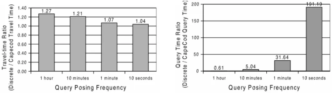
For each one of the two models we pose 100 queries. Regarding the discrete time model, each one of the queries runs multiple times for different degree of discretization. The query time interval for all the queries is set to 2 hours during the rush hours (during which the speed changes), while the Euclidean distance between the source and the destination node is about 7 to 8 miles. We compare the travel time and the query time of the two models. In both cases we use the ratio of the two measurements, i.e. Dis-crete Time model query time divided by CapeCod model travel time and Discrete Time model query time divided by CapeCod model query time respectively.
Figure 10(a) compares the travel time of the two ap-proaches while Figure 10(b) compares the query time for four different degrees of discretization. That is, for the dis-crete time model we pose a query every (i) 1 hour (ii) 10 minutes (iii) 1 minute and (iv) 10 seconds, within the query time interval. Posing a query every 1 hour results in around 1.27 times worse travel time compared to our method while the query time is better than the query time of our method. While the degree of discretization increases, although the travel time given by the discrete model approaches the travel time given by our model, the query time increases exponen-tial. Posing a query every 10 minutes results in 1.21 times worse travel time accuracy while making the discrete time approach 5 times slower than our approach. For the last de-gree of discretization, i.e. posing a query every 10 seconds, although the discrete model is accurate enough regarding the travel time, the query time is around 200 times worse than our approach.
7
Conclusions
In this paper, we addressed the problem of computing fastest paths over road networks with traffic speed pat-terns. We proposed the CapeCod patterns to capture real-life speed information. Moreover, we proposed and solved two variations of the fastest path query given a leaving (or arrival) time interval. These queries have direct real-life ap-plications. Our solutions to the queries are novel extensions to the A* algorithm. An interesting and novel contribution is the proposal of a new lower-bound estimator. Our al-gorithms were experimentally evaluated. The experimental results confirmed that our methods are more accurate and more efficient than straightforward approaches (e.g. the dis-crete time model). GIS systems like MapQuest can be im-proved by incorporating our ideas.
(a) Accuracy (b) Query Time Ratio
Figure 10. CapeCod vs. Discrete Time Model. Travel Time and Query Time comparison for different levels of discretization.
This paper opens many interesting and practical issues for future work. Most existing work on spatial queries (kNN, RNN, closest pairs, clustering, etc.) considers either the Euclidean distance or the shortest network distance. It is interesting to study the impact on these work if we consider the fastest travel time instead.
References
[1] I. Chabini. Discrete Dynamic Shortest Path Problems in Transportation Applications. Transportation Research Record, 1645:170–175, 1998.
[2] V. Chakka, A. Everspaugh, and J. Patel. Indexing Large Trajectory Data Sets With SETI. In Biennial Conf. on
Inno-vative Data Systems Research (CIDR), 2003.
[3] H. D. Chon, D. Agrawal, and A. E. Abbadi. FATES: Find-ing A Time dEpendent Shortest path. In ProceedFind-ings of the
4th International Conference on Mobile Data Management,
pages 165–180. Springer-Verlag, 2003.
[4] Y. Huang, N. Jing, and E. Rundensteiner. Spatial Joins Using R-trees: Breadth-First Traversal with Global Optimizations. In VLDB, pages 396–405, 1997.
[5] B. Jiang. I/O-Efficiency of Shortest Path Algorithms: An Analysis. In ICDE, pages 12–19, 1992.
[6] N. Jing, Y.-W. Huang, and E. A. Rundensteiner. Hierarchi-cal Optimization of Optimal Path Finding for Transporta-tion ApplicaTransporta-tions. In Proc. of Int. Conf. on InformaTransporta-tion and
Knowledge Management (CIKM), pages 261–268, 1996.
[7] N. Jing, Y.-W. Huang, and E. A. Rundensteiner. Hierarchical Encoded Path Views for Path Query Processing: An Optimal Model and Its Performance Evaluation. TKDE, 10(3):409– 432, 1998.
[8] S. Jung and S. Pramanik. HiTi Graph Model of Topograph-ical Roadmaps in Navigation Systems. In ICDE, pages 76– 84, 1996.
[9] F. Kamoun and L. Kleinrock. Hierarchical Routing for Large Networks: Performance Evaluation and Optimization.
Com-puter Networks, 1:155–174, 1977.
[10] R.-M. Kung, E. N. Hanson, Y. E. Ioannidis, T. K. Sellis, L. D. Shapiro, and M. Stonebraker. Heuristic Search in
Data Base Systems. In Expert Database Systems Workshop
(EDS), pages 537–548, 1984.
[11] K. Nachtigall. Time depending shortest-path problems with applications to railway networks. European Journal of
Op-erational Research, 83:154–166, 1995.
[12] A. Orda and R. Rom. Shortest-Path and Minimum De-lay Algorithms in Networks with Time-Dependent Edge-Length. Journal of the Association for Computing
Machin-ery (JACM), 37(3):607–625, 1990.
[13] A. Orda and R. Rom. Minimum Weight Paths in Time-Dependent Networks. Networks: An International Journal, 21, 1991.
[14] S. Pallottino and M. G. Scutell`a. Shortest Path Algorithms in Transportation Models: Classical and Innovative Aspects. In P. Marcotte and S. Nguyen, editors, Equilibrium and
Ad-vanced Transportation Modelling, pages 245–281. Kluwer
Academic Publishers, 1998.
[15] S. Russell and P. Norvig. Artificial Intelligence: A Modern
Approach. Prentice-Hall, Englewood Cliffs, NJ, 2nd edition
edition, 2003.
[16] S. Shekhar, A. Fetterer, and B. Goyal. Materialization Trade-Offs in Hierarchical Shortest Path Algorithms. In
SSTD, pages 94–111, 1997.
[17] S. Shekhar, A. Kohli, and M. Coyle. Path Computa-tion Algorithms for Advanced Traveller InformaComputa-tion System (ATIS). In ICDE, pages 31–39, 1993.
[18] S. Shekhar and D.-R. Liu. CCAM: A Connectivity-Clustered Access Method for Networks and Network Com-putations. TKDE, 9(1):102–119, 1997.
[19] K. Sung, M. Bell, M. Seong, and S. Park. Shortest paths in a network with time-dependent flow speeds. European
Journal of Operational Research, 121(1):32–39, 2000.
[20] J. L. Zhao and A. Zaki. Spatial Data Traversal in Road Map Databases: A Graph Indexing Approach. In Proc. of Int.
Conf. on Information and Knowledge Management (CIKM),