Usage of Road Weather Sensors for automatic traffic
control on motorways
Andrea Haug
1and Slavica Grosanic
21chair of traffic engineering and Control, Technische Universität München, Germany. 2Regierungspräsidium Tübingen, Germany.
[email protected], [email protected]
Abstract
Within section control systems on motorways drivers get information about adequate speed limits during adverse weather situations. Therefore road weather data are necessary. To detect the danger of aqua-planning measurements of precipitation intensity and waterfilm thickness as well as the status of the road surface are needed. To detect these atmospheric data different weather sensors are located near the motorway. There are two different sensor systems available which detect these measurements at the moment. For the detection of the status of the road surface, like dry, moist or wet, the sensor is embedded directly in the road surface in most cases. The other sensor system is non-invasive which can be installed next to or over the road. Nowadays more and more open-pored asphalt is used because of its advantage to be less noisy and its property to drain off water better than normal asphalt. But this kind of asphalt cannot be cut to install a road sensor therefore the usage of non-invasive sensors will increase in the future. This may also lead to different thresholds in automatic traffic control during adverse weather situations.
The measurements of waterfilm thickness, road surface and road temperature are very important for automatic traffic control algorithms [2] as a speed limit caused by rain is derived and shown on variable message signs. In the German Technical Bulletin [2] a matrix with the two measurements precipitation intensity and waterfilm thickness define which wetness-level is detected. There are 5 wetness-levels which cause different speed limits. For the first supply thresholds are given based on the experiences with road sensors. For the newer non-invasive sensors other thresholds may be necessary. This paper will show some possible thresholds for the precipitation/waterfilm thickness matrix and their effects on the speed limits shown on the variable message signs.
Within the German Test Site for Road Weather Stations [1] various road sensors as well as various non-invasive sensors are installed. The data for both detection technologies has been collected for the last 2 years and allows a statistically valid comparison of them. In this paper the advantage and disadvantage of the two sensor technologies will be shown for the measurements waterfilm thickness, road surface and road temperature. In order to describe the behavior of the sensors, the available data will be analyzed concerning the availability of valid datasets and the accuracy.
Keywords: road weather data, automatic traffic control algorithms, precipitation/waterfilm thickness matrix
Transportation Research Procedia
Volume 15, 2016, Pages 537–547
ISEHP 2016. International Symposium on Enhancing Highway Performance
1
Introduction
Weather sensors are used within the automatic traffic control to warn the driver of adverse weather situations. In the test site “Eching Ost” three embedded and three non-invasive sensors are installed. Both sensors determine plausible values and the overall results look similar but there are slightly different trends and values, which need to be analyzed to examine if the performance is the same and if there are any limitations for the usage of those types in traffic control systems on motorways. The ground truth is not always evident as there is no reference or the reference is very complex to include e.g. webcam pictures for every minute. Therefore most of the analysis is done by comparing the different sensor types to identify specific trends.
2
Sensor Types and Requirements
For detecting road temperature, waterfilm thickness and condition of the road surface the sensors can be divided into two types. There are non-invasive sensors which are either installed on poles or gantries next to or above the road. They are easy to install as the road does not need to be cut. Their usage is also possible on bridges and road surfaces that cannot be cut, e.g. open porous asphalt.
The measuring method used in these sensors is an optical spectroscopy which is either laser or infrared based. The road temperature is measured using a pyrometer. (www.lufft.de, 2015) (www.vaisala.com, 2015). For this study the non-invasive Sensors Lufft NIRS31, Vaisala DSC111 and Vaisala DST111 are used.
Embedded road sensors are located in the road either in the middle of a lane or underneath the tires on the left lane. They can additionally measure the temperature in different depths. The measuring method is either radar absorption based or thermic passive. (www.lufft.de, 2015) (www.vaisala.com, 2015) Used in this study are the sensors Lufft IRS31 and Vaisala DRS511. Both of them are located in the middle of the lane.
To ensure an adequate display there are requirements the sensors have to meet. Among the location which has to be homogeneous the sensors have to transmit a measured value every minute. Depending on the parameter there are specific requirements which are explained in the next section.
Sensors for road weather data should be located every 2-5 km. Variable message signs however are located closer. That is why the data needs to be very accurate as it is the input for more than one sign.
3
Usage in Traffic Control Systems
According to the TLS (2012) the sensors have to meet certain requirements to be used in automatic control algorithms for traffic management.
3.1
Condition of the Road Surface
The status of the road defines the qualitative coverage of the road surface. The sensors need to be able to distinguish the status “dry” and “not dry” which includes moist and wet. Additionally the status “frozen” has to be detected as well. The status of the road is mainly used to detect the danger of sleekness. The model uses the status of the road, the road temperature, dewing temperature and air temperature.
3.2
Waterfilm Thickness
Waterfilm thickness is defined as the moistening of the road with water or dilution (salt). It is based on a plain surface. Its range is from 0.01 to 3 mm. The value per minute has to be determined of six measurements within the last minute. The measurement of the waterfilm has a tolerance of 0 mm up to a waterfilm thickness of 0.19 mm. In between 0.2 mm and 0.49 mm the tolerance is 0.05 mm. Above 0.5 mm the tolerance is 0.1 mm.
There are four different levels for waterfilm thickness and five different levels for precipitation. They are combined to a matrix which contains four different moistness levels which are used in control algorithms. This is explained in chapter 4.5.
3.3
Road Temperature
The road temperature defines the temperature of the layer between the road surface and the air mass or the waterfilm above the road. The range needs to be from -30 to +80 °C and the resolution needs to 0.1 °C.
The Road temperature itself is not used for automatic traffic control but it is used as one of the main inputs to detect sleekness by using a specific model which is explained in (FGSV, 2010). Furthermore it is used to check the plausibility of other parameters, e.g. the status of the road. As those parameter influence the message signs, the accuracy of the road temperature is important. Additionally it is used to detect the danger of blow ups which occur of concrete surfaces exceed a temperature of > 35°C.
4
Comparison of Sensor Types
4.1
Data Collection
Near Munich on the motorway A92 is a test area for road weather sensors maintained by the federal government (Test site “Eching Ost”). The data has been observed continuously the whole year since 2004. There are different sensor types, concerning road weather for all parameters needed for traffic control systems. The parameters are recorded every minute. Additional there are webcam pictures which are also recorded every minute to get an impression about the weather and to benchmark the recorded data e.g. status of the road. For every meteorological year (November to Oktober) all sensors are benchmarked for the different parameters. (Rascher, Grosanic, & Busch, 2014)
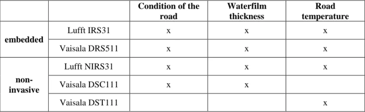
Used are the following sensors. Their location can be seen in Figure 1.
Condition of the road Waterfilm thickness Road temperature embedded Lufft IRS31 x x x Vaisala DRS511 x x x non-invasive Lufft NIRS31 x x x Vaisala DSC111 x x Vaisala DST111 x
Figure 1: Location of the Sensors
For this study data from November 2012 to October 2014 are used (about 1 million datasets). The data is checked according to its plausibility. The following four different types of plausibility checks are carried out for every measurement X(t).
- Threshold value: Xmin≤ X(t) ≤ Xmax (e.g. Waterfilm thickness: 0 mm ≤ X(t) ≤ 3 mm)
- Differential control: X(t) = X(t+1) = X(t+n); n = maximal duration with no change in time series (e.g. Road temperature: n = 60 Minutes)
- Rate of change: │X(t)-X(t-1)│≤Δrmax; Δrmax = maximal rate of change (e.g. Waterfilm
thickness: Δrmax = +/- 2 mm)
- Cross Correlation between two different measurements: e.g. status of road surface = “dry” and Waterfilm thickness > 0 mm, then both measurements are not plausible.
About 95 % of the datasets for the analyzed two years are available. 5 % of data is missing due to data logging. Only 1 % of data is marked as not plausible. Data was only used when all considered sensors delivered plausible data in the minute interval. Waterfilm thickness is compared as a subject to road temperature using the sensor DRS511. Therefor the minute interval is only used if all values for waterfilm thickness and temperature are plausible.
4.2
Condition of the Road
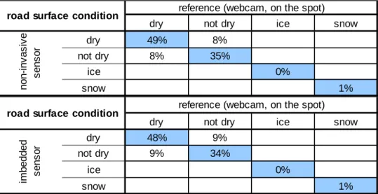
The status of the road is evaluated by comparing the status given by the sensor to what is seen on the webcam pictures. The sensors usually recognize the right status especially the change from “dry” to “not dry”. Additionally on-site observations are carried out. In the following diagrams the recognized road surface condition of the sensor and the corresponding recognized condition of road surface of the reference, which are either webcam pictures or an observer on-site, can be seen. According to (BASt, 2012) the status is subdivided in classes dry, not dry, ice and snow. As it is difficult to determine the exact condition of the road by looking at very short intervals, e.g. one picture, a longer period (T > 5 Minute) is determined and also the location of the sensor is considered. For this study a total number of 184 events is considered. As it can be seen in Table 2 there is a high correspondence between the observer and the sensor.
Table 2: Comparison of the road surface condition determined by the sensor to a reference
Because longer periods are usually evaluated slightly different than short periods, as the overall trend is the same, some specific short occurrences are not taken into account. The drying process, for example, is different between the two sensor types. Figure 2Fehler! Verweisquelle konnte nicht gefunden werden. shows an example of a random rain event with medium intensity from May 2013.
Figure 2: Correlation of waterfilm thickness and road surface condition
As it can be seen the embedded sensors have a quicker drying process than the non-invasive sensors, which is especially seen in the wet condition. First the waterfilm thickness is decreasing faster and therefore the condition of the road surface changes faster. This is especially important for the acceptance
dry not dry ice snow
dry 49% 8%
not dry 8% 35%
ice 0%
snow 1%
road surface condition reference (webcam, on the spot)
non-inv as iv e s ens or
dry not dry ice snow
dry 48% 9%
not dry 9% 34%
ice 0%
snow 1%
road surface condition reference (webcam, on the spot)
im bedded sens or -1 -0.5 0 0.5 1 1.5 06:00 07:00 08:00 09:00 10:00 11:00 12:00 13:00 14:00 15:00 16:00 17:00 W aterfilm thickness [mm] 29.05.2013 Condition of road surface non-invasive sensor embedded sensor dry
not dry (wet) not dry (moist)
non -invasive sensors
embedded sensors
of traffic control systems, as the user wants to be able to recognize the shown displays in his environmental surroundings. If this is not plausible the displayed sign might not be accepted. Many drivers tend to not accept the displays, even if they reflect the environmental conditions, when they show a high rate of non-plausible displays. For those reasons it is recommended to install a good calibrated sensor and to adapt the traffic management algorithm according to the sensor. Within this process local conditions of the sensor location have to be included as well.
4.3
Waterfilm Thickness
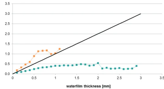
Concerning the waterfilm thickness the ground truth is not known in general. (Grosanic & Grötsch, 2010) developed a procedure to measure the waterfilm thickness with towels. It is used in the test site to determine the accuracy of the sensors. Other procedures like the use of a “spraying box” (Grosanic & Busch, 2010) are also known. Those tests have in common, that they are extensive as a road closure is needed, and therefore there are only a few tests per year possible. Additionally every test is done for a specific sensor, hence all tests have a specific waterfilm and cannot be compared directly to see if one sensor type reacts in a specific way. In order to identify the difference between each sensor the difference in waterfilm thickness is calculated. Figure 3 shows the standardized sum of positive and negative deviation of the embedded road sensors to the non-invasive sensors. It can be seen, that the deviation is increasing as the waterfilm thickness increases. It can also be seen, that the negative deviation is bigger than the positive deviation, which means, that the embedded sensors determine smaller waterfilm thicknesses than non-invasive sensors which might be due to the quicker drying process and the method of measuring the waterfilm thickness. This fact becomes apparent when the waterfilm thickness is above 0.6 mm. There are no positive deviations above 1.1 mm. This figure only shows the trend of the deviations for each waterfilm thickness step of 0.1 mm (big squares). The absolute quantity of values for each deviation step is not displayed in the figure but the total quantity of values for the negative deviation is above 70 % of all deviations for waterfilm thicknesses above 0.2 mm and above 90 % for waterfilm thicknesses above 0.6 mm.
As the ground truth is not known, it is not known which sensor type performs better. However in certain situations when the temperature is around 0 °C it is important to detect the right waterfilm thickness to warn the driver against slippery or icy roads and to coordinate the winter services. To analyze if the sensors have a better correlation within the critical range the waterfilm thickness is merged with the road temperature. The value of the waterfilm thickness of the two different sensor types is compared according to the range of tolerance described in 3.2. The quantity in percentage is calculated within the tolerance range and when the embedded sensor is outside the range of tolerance of the non-invasive sensor. The results are displayed in Figure 4. It can be seen, that there is no evident correlation between the temperature and the waterfilm thickness. The sensors determine only values within the range of tolerance for small waterfilm thicknesses. Above 0.7 mm there are hardly any intervals within the range of tolerance. As described above, the higher the waterfilm thickness gets the deviation of the sensors gets out of the range of tolerance negatively. Positive values outside the range are mainly found within waterfilm thicknesses up to 0.6 mm. Which means that if the waterfilm thickness increases above 0.6 mm it is very likely that the non-invasive sensor determines a higher value than the embedded sensor.
Figure 4: waterfilm thickness dependent on road temperature
4.4
Road Temperature
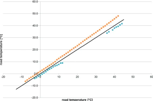
In order to detect the differences of the sensor types for measurement of the road temperature the standardized sum of the deviation was calculated for all sensor pairs. The sensors are counted to have the same value if the difference is smaller than +/- 1 degree in the critical range from -8 °C to +8 °C. In all other ranges the values are counted as “same” if the difference is smaller than +/- 2 degree. The critical range is chosen because within these temperatures the road condition can change very fast. If it is moist on the road it can get slippery or icy. This range of temperature is more important for traffic management than the boundary area of the temperature spectrum.
Figure 5: road temperature deviation of an embedded sensor to a non-invasive sensor
Figure 5 above shows the standardized sum of positive and negative deviation of the non-invasive sensors to the embedded road sensors. Mostly the embedded sensor shows higher road temperatures than the non-invasive sensor. The higher the temperature gets the bigger the deviation gets. In the range between -3°C and +12°C the number of positive and negative deviation is nearly the same. With increasing road temperature it becomes evident, that the embedded sensor determines higher values. The missing values in the negative deviation is because in this range the measured road temperatures are within the tolerance of +/- 2 degree. Therefore the number, when the sensor pair has the same value was also calculated. Figure 6 shows the percentage of same samples within the same minute interval. Although the sensors show the same trend in road temperature, the quantity of same values is very low. This raises the question if the tolerance ranges are too tight.
Figure 6: Quantity of same samples for road temperature
0.0% 0.5% 1.0% 1.5% 2.0% 2.5% 3.0% 3.5% 4.0% -13 -11 -9 -7 -5 -3 -1 1 3 5 7 9 11 13 15 17 19 21 23 25 27 29 31 33 35 37 39 41 43 45 Quantity [% ] road temperature [°C] 0 5 10 15 20 25 30 35 0:00 4:00 8:00 12:00 16:00 20:00 0:00 road temperature [° C] time [hh:mm] embedded sensor non-invasive sensor
4.5
Usage in Traffic Control Algorithms
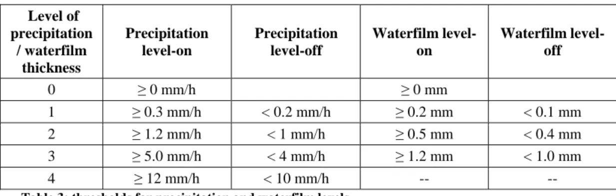
The measurements of water film thickness and precipitation are used to calculate the level of moistness for every minute. In a first step the plausibility checked data is categorized into different levels of wetness. Table 3 shows the thresholds given in (FGSV, 2010). They can be used to get a first impression of the situation and to create an initial input for the control algorithm. Depending on the road surface it is recommended to check the outcome and to adapt the thresholds if necessary.
Level of precipitation / waterfilm thickness Precipitation level-on Precipitation level-off Waterfilm level-on Waterfilm level-off 0 ≥ 0 mm/h ≥ 0 mm 1 ≥ 0.3 mm/h < 0.2 mm/h ≥ 0.2 mm < 0.1 mm 2 ≥ 1.2 mm/h < 1 mm/h ≥ 0.5 mm < 0.4 mm 3 ≥ 5.0 mm/h < 4 mm/h ≥ 1.2 mm < 1.0 mm 4 ≥ 12 mm/h < 10 mm/h -- --
Table 3: thresholds for precipitation and waterfilm levels
In the next step the moistness level is defined with the following matrix. According to the level of moistness the speed limits are defined according to Table 5.
Level of precipitation 0 1 2 3 4 No data Lev el of wa ter film thicknes
s 0 dry dry wet 1 wet 2 wet 2 dry
1 wet 1 wet 1 wet 2 wet 3 wet 4 wet 1
2 wet 2 wet 2 wet 2 wet 3 wet 4 wet 2
3 wet 2 wet 2 wet 3 wet 3 wet 4 wet 3
No data dry dry wet 1 wet 2 wet 3 Table 4: definition of moistness level
Variable message sign Level of moistness
Wet 1
Wet 2
Wet 3
Wet 4 Table 5: variable message signs according to level of moistness
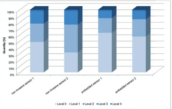
Figure 7 shows the quantity of the levels of moistness that would have been used for the displays in the control algorithm as it is explained above. The sensor Thies Laser Niederschlagsmonitor was used as reference for the precipitation intensity. Data sets were only used if all sensors delivered data for the minute interval. The quantity of each level is similar regardless of which sensor type is used. The level of moistness 1 and 2 is influenced by the waterfilm thickness and the precipitation intensity. Moistness Level 3 and 4 is mainly influenced by the precipitation intensity as the waterfilm thickness itself has already reached the highest level. The total quantity of values within these levels is low and no evident differences between the sensor types can be seen. Therefor the following figure only allows to draw conclusions on the waterfilm thickness for level of moistness 1 and 2. The quantity of level 0 is smaller for non-invasive sensors. They react more sensible and recognize a waterfilm quicker. That is also why the quantity of moistness level 2 is higher. Non-invasive sensors react differently during the drying process. They show waterfilm thicknesses longer than embedded sensors. The values stay longer in the waterfilm level 1 and therefor also moistness level 1.
Figure 7: Quantity of levels of moistness
As shown in figure 4 the non-invasive sensors show higher water film thickness than the embedded sensor for values above 0.8mm which would be the level of moistness 2, 3 or 4 depending on the precipitation intensity. Figure 7 shows that the quantity of the level of moistness 2 is higher for non-invasive sensors.
In order to show adequate speed limits on the displays it might be useful to choose lower thresholds for the level of moistness when using non-invasive sensors. As the sensors show a wide range of results it is very important to check the environmental conditions for every sensor because they have a huge influence on the measurements of the sensor.
5
Conclusion
Even if the overall trends and values look similar the analysis show, that they are quite different and the tolerances defined in the guidelines are often not met. As the sensors get evaluated as “suitable for the usage in traffic control systems” in (Rascher, Grosanic, & Busch, 2014), further study should be done in assessing the required tolerance ranges. Because the ground truth is not known in general for all events, especially waterfilm thickness and road temperature, it is not possible to identify the sensor type which determines the better values. However, this paper shows the differences between the sensor types which need to be considered within the operation of traffic control systems. In this paper it was shown, that for the condition of the road the sensor types are similar concerning the comparison to the reference however there are differences in the drying process. The analysis of the waterfilm thickness showed, that embedded sensors determine smaller values than non-invasive sensors with rising waterfilm thickness. It is the other way round for road temperature. There the embedded sensors determine greater values. It is recommended to choose lower thresholds to determine the level of moistness in order to display adequate speed limits.
References
BASt. (2012). Technische Lieferbedingungn für Streckenstationen (TLS). Bergisch Gladbach: Bundesanstalt für Straßenwesen.
FGSV. (2010). Hinweise für die Nutzung von Umfelddaten in Streckenbeeinflussungsanlagen. FGSV Verlag, Köln.
Grosanic, S., & Busch, F. (2010). Umfelddatenerfassung in Streckenbeeinflussungsanlagen, Testfeld "Eching Ost" des Bundes, Abschlussbericht 5. Testphase. München.
Grosanic, S., & Grötsch, S. (2010). Anleitung zur Ermittlung der Wasserfilmdicke auf der Fahrbahn mittels eines Tuchtests im Umfelddatentestfeld des Bundes. München.
Rascher, A., Grosanic, S., & Busch, F. (2014). Umfelddatenerfassung in Streckenbeeinflussungs-anlagen, Testfeld "Eching Ost" des Bundes, Abschlussbericht 9. Testphase. München. www.lufft.de. (2015, 09. 09).