Testing Affine Term Structure Models in Case of Transaction Costs

(1)

Testing Affine Term Structure Models in case of

Transaction Costs

Joost Driessen

Bertrand Melenberg

Theo Nijman

First Version: November 26, 1998

This Version: September 15, 1999

We thank Lars Hansen, Pieter-Jelle van der Sluis, Bas Werker and participants of the Workshop Financial Modeling and Econometric Analysis, Lille 1999, and of the EFA conference, Helsinki 1999, for their helpful comments.

All three authors are from the Department of Econometrics, Tilburg University. Corresponding author: Joost Driessen, Department of Econometrics, Tilburg University, PO Box 90153, 5000 LE Tilburg, The Netherlands. Tel: +31-13-4663219. E-mail: [email protected].

(2)

Testing Affine Term Structure Models in case of

Transaction Costs

Abstract

In this paper we empirically analyze the impact of transaction costs on the performance of affine interest rate models. We test the implied (no arbitrage) Euler restrictions, and we calculate the specification error bound of Hansen and Jagannathan to measure the extent to which a model is misspecified. Using data on T-bill and bond returns we find, under the assumption of frictionless markets, strong evidence of misspecification of one- and two-factor affine interest rate models. This is in line with earlier research. However, we show that the pricing errors of these models are reduced considerably, if relatively small transaction costs are taken into account. The average transaction costs for T-bills, due to the bid-ask spread, are around 1.5 basis points. At this size of transaction costs and for monthly holding periods, the misspecification of one- and two-factor affine interest rate models becomes statistically insignificant and economically very small. For quarterly holding periods, higher transaction costs of around 3 basis points are required to avoid misspecification.

JEL Codes: G12, E43.

(3)

1 Introduction

Nowadays term structure models are used extensively for many purposes, including risk management of portfolios containing bonds and the valuation of interest-rate derivatives. Not surprisingly, tests of the empirical validity of the commonly used term structure models have attracted considerable attention in the literature. In line with a large part of the empirical asset pricing literature, the tests are based on the assumption of trading in frictionless markets. For example, Stambaugh (1988), Gibbons and Ramaswamy (1993), and Pearson and Sun (1994) test affine interest rate models using data on Treasury bills and bonds under the assumption of trading in frictionless markets. However, market frictions such as transaction costs or short selling constraints are an important fact of life for investors. The implicit assumption when ignoring transaction costs is that these costs are sufficiently small, so that they do not seriously affect the empirical results. In this paper we will explicitly take transaction costs into account in the empirical testing of affine term structure models, and show that including transaction costs considerably affects tests of affine interest rate models.

We shall analyze the interest rate models by testing whether the stochastic discount factor of each of these interest rate models satisfies the Euler restrictions. These Euler restrictions are implied by the no-arbitrage assumption, and can be derived in both frictionless markets and markets with frictions. Based on these Euler restrictions, we will use two approaches to analyze and test the models. First, we use Wald-type tests to test the implied Euler restrictions. For the frictionless case, the analysis of Euler restrictions using Wald-tests is extensively discussed by Cochrane (1996). A disadvantage of this approach is that, if one rejects a model, there is no clear indication of the direction of misspecification, for example which individual assets are possibly mispriced by the model and which are not. Also, if one applies this approach to two non-nested models and both are rejected, no indication is obtained whether one model is more misspecified than the other. To overcome these problems we also consider the specification error bound (SEB) developed by Hansen, Heaton and Luttmer (1995) and Hansen and Jagannathan (1997). This bound measures the extent to which a model misprices a given set of assets. Hansen and Jagannathan (1997) show that this bound can be interpreted as the maximum pricing error for all portfolios that can be constructed from the assets under consideration. Also, this specification error bound allows for direct comparison across (non-nested) models and the method indicates which (portfolios of) assets contribute most to the misspecification. Hansen and Jagannathan (1997) only consider frictionless economies; Hansen, Heaton and Luttmer (1995) extend the setup to allow for market frictions. We apply their approach to affine term structure models and compare the results with standard tests using the Euler restrictions.

Our work is related to Luttmer (1996) and He and Modest (1995), who both analyze the influence of transaction costs and other market frictions on the size of the volatility bounds of Hansen and Jagannathan (1991), that give a lower bound on the variability of valid stochastic discount factors. Empirically, Luttmer (1996) finds that small transaction costs greatly influence the size of the volatility bounds; especially, the

(4)

volatility bounds based on T-bill returns are very sensitive to the size of transaction costs. The results of Luttmer (1996) imply that the conclusion of rejection of several asset pricing models in Hansen and Jagannathan (1991), based on the volatility bounds, changes if transaction costs are taken into account. Our work extends the work of Luttmer (1996), because the volatility bound is a special case of the specification error bound. Also, Luttmer (1996) focuses on consumption-based asset pricing models, whereas we analyze bond pricing models and bond returns.

The bond pricing models that we consider are discrete-time versions of the affine-yield models of Duffie and Kan (1996). This class includes the well-known Vasicek (1977) and Cox, Ingersoll and Ross (CIR, 1985) models. There is by now a large literature that empirically investigates these affine-yield models in frictionless markets (for example, Babbs and Nowman (1999), Backus and Zin (1994), Brown and Schaefer (1994), Chen and Scott (1993), Gibbons and Ramaswamy (1993), De Jong (1999), and Pearson and Sun (1994)). Our results indicate that, without market frictions, there is considerable evidence that both one- and two-factor Vasicek, CIR and general affine Duffie-Kan (1996) models significantly misprice the returns on bond portfolios, and, especially, the returns on portfolios that contain both extreme long and short positions in short-maturity T-bills. This result is in line with most of the empirical work mentioned above, although in this literature the results for two-factor models are somewhat mixed. We also find that the factor Vasicek and CIR models have much higher specification errors than the general affine two-factor model.

After investigating the frictionless case, we analyze how the empirical results are affected if transaction costs are taken into account. The average bid-ask spread for T-bill prices in our data is approximately 3 basis points, which is of a similar size as the spread reported by Luttmer (1996). We find that, for monthly holding periods, the bond pricing implications of the one- and two-factor affine models are consistent with the data for transaction costs of only 1.5 basis points: the misspecification of the simple one- and two-factor models is then both statistically insignificant and economically very small. Because of the transaction costs, the portfolios with both long and short positions in T-bills (and bonds) are no longer mispriced. For quarterly holding periods, on the contrary, the one- and two-factor affine models are rejected at the same size of transaction costs. Transaction costs around 3 basis points are required in this case to avoid any evidence of model misspecification.

The remainder of this paper is organized as follows. In section 2, we briefly review the literature on affine interest rate models and asset pricing in markets with frictions. In section 3, we describe a Wald-test of the Euler restrictions in a market with frictions. Section 4 discusses the specification error bound. In section 5, we describe our data as well as the parameter estimates for the affine interest rate models. In section 6 we present the empirical results for the Wald-tests and specification error bound both for the one-and two-factor models. In section 7 we summarize one-and conclude.

(5)

E_t[R_i_,_t_%₁Y_t_%₁] ' 1, i'1,..,n. ₍₁₎ E_t[R_i_,_t_%₁Y_t_%₁] # 1, i'1,...,n, ₍₂₎ (1&s/2) P_i_,_t_%₁ (1%s/2) P_i_,_t / J l Pi,t%1 P_i_,_t / J l_R i,t%1, (3) (1%s/2) P_i_,_t_%₁ (1&s/2) P_i_,_t / J s Pi,t%1 P_i_,_t / J s_R i,t%1. (4)

2 Pricing Implications of Affine Interest Rate Models in

case of Transaction Costs

Let the n-dimensional vector Rt+1 contain the monthly gross returns from time t to time t+1 of n assets (in

our case bonds of n different maturities). Without market frictions, it is well known (see, for example, Campbell, Lo and MacKinlay (1997), Chapter 11) that absence of arbitrage opportunities in terms of the n assets requires the existence of a strictly positive stochastic discount factor (SDF) Yt+1 satisfying

Here the expectation is conditional on the information set at time t. A model formulated in terms of a particular SDF can be tested by verifying some implied unconditional version of equation (1).

If there are short-selling constraints on the assets, absence of arbitrage opportunities requires the existence of a strictly positive SDF satisfying

see, for example, Jouini and Kallal (1995) or Luttmer (1996). For any given SDF Yt+1, these Euler

inequalities can be tested by applying, for example, the methodology of Kodde and Palm (1986). When considering transaction costs, we restrict ourselves to the case of a proportional spread s that is equal at the ask and bid side, and the same for all assets under consideration. Let P_i_,_t denote the midprice of asset i at time t. Then the gross return on taking a long position is equal to

(6)

1

In Campbell, Lo and MacKinley(1997), the specification of the log-SDF also contains a normally distributed variable that is independent from >. This variable only influences the mean of the yield curve in a way that is very similar to the way the mean of the state-variable influences the mean yield curve. In our analysis we do not include this variable (in line with Backus and Zin (1994), Backus et al. (1997) and Bansal (1998)), allowing us in a straightforward way to calculate the SDF in terms of observables.

1 Js # Et[Yt%1Ri,t%1] # 1 Jl, i'1,...,n. (5) &y_t_%₁ ' 4) Nxt%()>t%1 x_t_%₁ ' µ%7x_t%E>_t_%₁ >_t_%₁|I_t ~ N(0,V) V ' diag($₁%") 1xt,....,$N%")Nxt). (6) In testing, transaction costs can be taken into account by rewriting the problem as one with restrictions on short and long positions (see Luttmer (1996)) and introducing separate assets for a long position in asset i with return JlR_i_,_t_%₁ and for a short position with return JsR_i_,_t_%₁. As a consequence, the absence of arbitrage opportunities in the presence of transaction costs requires the existence of a strictly positive SDF Yt+1 such that

We will analyze affine interest rate models using the Euler restrictions in (5), by testing whether the SDF that is implied by an affine model satisfies these restrictions for bond returns, where we shall consider different values of Jl and Js.

Duffie and Kan (DK, 1996) describe the class of continuous-time multi-factor interest rate models, that imply an affine relationship between interest rates and a vector of state variables. Our setup is in discrete time. Therefore, we will use discrete-time versions of these models, as described by, for example Backus et al. (1997) and Campbell, Lo and MacKinley (1997). These authors show that a discrete-time term structure model is affine, if the one-period ahead conditional joint distribution of the log-SDF, , and an N-dimensional vector of state variables is multivariate normal, and the

y_t_%₁ ' log(Y_t_%₁) x_t_%₁

conditional expectation and covariance matrix are both affine functions of the state-variables . Therefore,x_t the N factor discrete-time DK model with conditionally normal innovations can be written as1

Here >_t_%₁ represents an N-dimensional conditionally normally distributed random vector with zero conditional mean and conditional variance matrix V, 7 and G are N×N-matrices containing unknown parameters, "₁,...,"_N, $ ' ($₁,...,$_N)), µ, and ( are N-dimensional unknown parameter vectors, 4_N is an

(7)

2

Furthermore, not all parameters in these affine models are identified. Following Dai and Singleton (1997), we normalize the Vasicek and CIR models by setting G equal to the identity matrix, and by imposing that the matrix 7 is a diagonal matrix. Moreover, in the Vasicek model we normalize by setting all elements of the vector µ equal to zero, except for the first element µ1.

&logP_nt ' n r_nt ' A_n%B_n)x_t, (7)

>_t_%₁ ' E&1₍_x

t%1&µ&7xt) (8)

&y_t_%₁ ' &()_E&1_µ_%₍₄)

N&()E&17)xt%()E&1xt%1 (9)

&y_t_%₁ ' 2₁%2)

2rtx%2)3rt%x1 (10)

N-dimensional vector containing ones, and represents the information set of time I_t t. The components of the vector ( can be interpreted as the market prices of risk, as they measure the sensitivity of the SDF (and thus bond returns) for the underlying factors. The N-factor Vasicek model is obtained by setting , whereas the N-factor CIR model is obtained if .2

"_j ' 0, j'1,..N $_j ' 0, "_j'(0, .., 0,"_jj, 0, ..., 0)), j'1,..N

In the empirical analysis, we will present results both for one- and two-factor Vasicek and CIR models and for general affine one- and two-factor models.

Using equations (1) and (6), one can derive that bond prices are exponential-affine functions of the state variable xt,

where Pn,t is the price of an n-period zero-coupon bond at time t, and rnt is the corresponding interest rate.

The factor loadings An and Bn are functions of the underlying parameters, and do not depend on time. By

rewriting (6) the SDF can be expressed in terms of observables. First, by substituting >t+1 in equation (6),

we get

and, thus, the SDF is given by

Because all interest rates are affine functions of the state-variables, as shown in equation (7), this relationship can be used to obtain a log-SDF that is affine in interest rates of N different maturities and their lagged values. If we define r_tx as the N-dimensional vector containing these N interest rates, the SDF becomes

(8)

Y_tk ' k k j'1 Y_t_%_j, R_i_,k_t ' k k j'1 R_i_,_t_%_j. (11)

where the parameter 21, and the N-dimensional vectors 22 and 23 are implicitly defined. Hence, these

reduced form parameters 2 ' (2₁,2₂),2₃))) are functions of the structural parameters in equation (6). Equation (10) gives the functional form of the SDF that is implied by the discrete-time DK model (6) with conditionally normally distributed innovations. As noted by Kan and Zhou (1999), even if the SDF in (10) satisfies the Euler restrictions exactly, there are other SDFs that also satisfy the Euler restrictions. Testing whether a stochastic discount factor satisfies the Euler restrictions does not require a fully specified equilibrium model for asset returns. The advantage of testing Euler restrictions is, therefore, that one can test a large class of models without making very specific assumptions. In our case, we can test all affine term structure models with a given number of factors, by using the Euler restrictions both to estimate the reduced-form parameters 2 and to test the specification of the SDF in (10). Khan and Zhou (1999), demonstrate that, if estimation and testing are based on Euler restrictions only, the test procedure might have low power in detecting misspecified models. Therefore, we will also analyze specific equilibrium models, namely the Vasicek and CIR models, by estimating the structural parameters of these models using other moment restrictions. These moment restrictions are derived from the specification of the Vasicek and CIR models in equation (6). Given estimates of the structural parameters of the Vasicek or CIR model, we can directly construct estimates for the reduced-form parameters 2 and construct the SDF of the Vasicek or CIR model using these parameter estimates. Subsequently, we test whether this Vasicek (or CIR) SDF satisfies the Euler restrictions.

In the next sections, we will use the pricing implications of affine term structure models as described above to test the empirical validity of these models, using Wald tests as well as the specification error bound of Hansen and Jagannathan (1997).

3 Testing the Euler Restrictions using a Wald-Test

For every affine term structure model, Wald-type tests of the Euler restrictions for both the frictionless case (equation (1)) and the case with transaction costs (equation (5)) are relatively straightforward to implement. For the case of transaction costs, the inequality constraints can be tested along the lines of Kodde and Palm (1986). In this section, we briefly review this test. The test for frictionless markets is a special case.

We analyze results for different holding periods, and, therefore, we first of all introduce products of monthly SDFs and monthly returns

(9)

1 Js # Et[Y k t Ri,kt] # 1 Jl, i'1,...,n. (12) 1 Js # E[Y_tkx_i_,k_t] E[q_t_,_i] # 1 Jl, i'1,...,m×n. (13) ˆ v_i / 1 Tj T t'1 Ytkxi,kt 1 Tj T t'1qi,t , i'1,...,n. ₍₁₄₎

In the empirical analysis, we will analyze both monthly and quarterly holding periods, i.e., values for k of, respectively, 1 and 3. Equation (5) implies that these lower frequency SDFs and returns satisfy

Following Hansen and Jagannathan (1991) and many others, we incorporate conditional information by constructing returns on managed portfolios with payoffs x_tk ' z_t¼R_tk and corresponding prices , where zt is a m-dimensional vector with variables that are in the information set at time t. The

q_t ' z_t¼4

implied unconditional Euler restrictions are

In general, this ‘multiplicative’ approach is not an optimal way of incorporating conditional information. For the volatility bounds of Hansen and Jagannathan (1991), Ferson and Siegel (1998) discuss how to use conditional information optimally. Because similar results do not seem to be available yet for the specification error bound, and because of the simplicity of the multiplicative approach, we prefer to use this approach. In the sequel we refer to x_tk as the vector of returns, and we denote the number of returns in (13) by n, instead of m×n, to avoid too cumbersome notation.

The null hypothesis is that the SDF satisfies the Euler restrictions (13). Given T time-series observations on the n-dimensional vector of returns x_tk and a SDF, we estimate the ratio of expectations in (13) by its sample analogue

(10)

3

We have also estimated the matrix W using Newey-West (1987) with 10 lags. This hardly changes the empirical results.

4

As suggested by Wolak (1989, 1991), we interpret this test as a local test of the inequality constraints. A global interpretation of our test procedure would imply that we overestimate the size of transaction costs that is needed to avoid statistical rejection of the model, or equivalently, that we would underestimate the influence of transaction costs on model misspecification.

5

We do not re-estimate the parameter vector 2 when we test the Euler restrictions in markets with transaction costs, because this complicates the calculation of the limit distribution of the test-statistic in (15). This is consistent with estimation strategy for the parameters of the Vasicek and CIR models, where the (structural) parameters are also not re-estimated in case of transaction costs.

>_w ' min_v_0ún T( ˆv&v))Wˆ&1 ( ˆv&v)

s.t. 1

Js # vi #

1

Jl, i'1,...,n,

(15)

where Wˆ is an estimator of the asymptotic covariance matrix of vˆ ' ( ˆv₁,..., ˆv_n)). For quarterly holding periods, we use the Newey-West (1987) method with 2 lags in order to correct for the overlapping nature of the quarterly pricing errors3_.

In the absence of transaction costs, the test-statistic >_w reduces to the J-statistic of Hansen (1982), and follows asymptotically a chi-square distribution with n degrees of freedom. In case of transaction costs, Kodde and Palm (1986) show that, under the null hypothesis, this test-statistic is asymptotically distributed as a mixture of chi-square distributions4_{. In this case simulation can be used to obtain p-values for a given}

value of the test-statistic.

A disadvantage of this testing methodology is that, if a model is rejected, there is little indication of the direction of the misspecification. Also, if one rejects two non-nested models, no indication is obtained whether one model is more misspecified than the other. In the next section, we will argue that the use of the specification error bound overcomes these problems.

As described in the previous section, we will both test fully specified conditionally normal Vasicek and CIR models, as well as the general class of affine term structure models. To test all affine models with a given number of factors, we estimate the parameters 2 in equation (10) by minimizing equation (15), with , over 2 as well5_{. Subsequently, we use the Wald-test statistic (15) to test the (overidentifying)}

Js_'_Jl_'₁

Euler restrictions, both for the frictionless markets case and the case of transaction costs. The estimation strategy for 2 lowers the number of degrees of freedom of the limit distribution, so that the results of Kodde and Palm (1986) are not directly applicable anymore. In the appendix we therefore derive the limit distribution of the Wald test-statistic in (15), given the estimation strategy for 2.

(11)

E[q_t_,_i] Js # E[m k t xi,kt] # E[q_t_,_i] Jl , i'1,...,n. (16)

However, given the number of factors, this test does not indicate which term structure model has the best empirical performance. Therefore, as described in the previous section, we also test the Vasicek and CIR models, which are special cases of the DK-class of conditionally normal affine models in equation (6). To analyze these models, we first derive moment restrictions that reflect the cross-sectional and dynamic implications of the models, and estimate the structural parameters of the models using GMM for these moment restrictions. These structural parameter estimates are then used to obtain estimates of the reduced form parameters in the SDF. Subsequently, we test whether the SDF of the Vasicek or CIR model satisfies the Euler equations using the test-statistic in (15). Because the moment restrictions that are used in the first step to estimate the parameters of the SDF are different from the Euler restrictions used in the second step to test the model, the number of degrees of freedom of the limit distribution of the test-statistic in (15) does not change. In this case, we only have to correct for the estimation of 2 in the calculation of the asymptotic covariance matrix in (15).

4 Analyzing the Euler Restrictions using the Specification

Error Bound

As stressed by Hansen and Jagannathan (1997), an asset pricing model is an approximation of reality and, therefore, it will typically not exactly satisfy the Euler restrictions in an empirical analysis. They propose to measure the size of misspecification of a given proxy model, with SDF Yt, by measuring in some way

the pricing errors of this proxy model. In this section, we briefly describe the part of their approach that is relevant for our application.

In our case, the proxy model is given by one of the models that we described in section 2. For a given holding period k, we start by introducing the set M of admissible SDFs consisting of random variables mt

k

(which are in the information set at time t+k) that satisfy the Euler restrictions

A SDF is thus admissible if it prices all (linear combinations of) the assets under consideration correctly. The SDF Yt

k_{that is associated with the proposed model can be used to calculate model prices of the}

payoffs, that, in general, may not satisfy the restrictions in (16). Hansen and Jagannathan (1997) propose to measure the size of this misspecification by

(12)

6

Hansen and Jagannathan (1997) also introduce a bound where the set of admissible SDFs only contains SDFs with the same unconditional mean as the proxy SDF, and show that this condition is automatically satisfied if one analyzes models with a stochastic discount factor that contains an additive, unknown constant term, that is chosen such as to minimize the SEB. We do not analyze stochastic discount factors with this property, and we also do not impose this restriction on the mean of the SDF, because this would imply that any model that we analyze prices the return of a one-period bond without error.

*2 _' _min

mtk0M E[(Y k

t &mtk)2]. (17)

* ' max_ë _{0 ú}n min_v_0ún |E[Y_tk(8)x_tk)&8)v]|

s.t. E[(8)x_tk)2] ' 1 E[q_t_,_i] Js # vi # E[q_t_,_i] Jl , i'1,...,n. (19) * ' max_ë_0ún |E[Y_tk(8)x_tk)&8)q_t] | s.t. E[(8)x_tk)2] ' 1 (18) The square root of (17) is called the Specification Error Bound (SEB), and can be interpreted as a (minimum) distance between the proxy SDF Yt

k_{and the set of admissible SDFs.}6

For the case without market frictions, Hansen and Jagannathan (1997) show that the SEB following from equation (17) has an interpretation as the maximal pricing error of all portfolios in the n assets

It is easy to show that this interpretation of the SEB still holds in the case of transaction costs. More precisely, given the set M defined by (16), one can show that * satisfies

This shows that * gives a bound on pricing errors of portfolio payoffs that are normalized in a particular way. Note that this normalization does not imply that the components or ‘weights’ in 8, which are equal to the Kuhn-Tucker multipliers of the binding Euler restrictions (see Hansen and Jagannathan (1997)), sum up to one.

A slight modification of a frictionless result in Hansen and Jagannathan (1997) reveals that the SEB can also be calculated as follows

(13)

7

If the true * is equal to zero, Hansen, Heaton and Luttmer (1995) argue that the limit distribution is mixed chi-square if there are no transaction costs. Then, this test-statistic is less efficient than the Wald-test discussed in the previous section.

8

Of course, the asymptotic variance as reported in Hansen, Heaton, and Luttmer (1995) has to be adjusted if the parameters of the SDF are estimated in the first step.

*2 _' _min

v0ún E[Y k

t xtk&v])E[xtkxtk)]&1E[Ytkxtk&v]

s.t. E[qt,i]

Js # vi #

E[q_t_,_i]

Jl , i'1,...,n

(20)

*2_min ' min_è₀_È max_mk

t0M E[(Y k

t (2)&mtk)2], (21)

Comparing this with equation (15) shows that the SEB is closely related to the population analogue of the Wald test-statistic. The only difference is the weighting matrix. Below we return to this difference and to the relative advantages of the two approaches.

By replacing population moments with their sample analogues in equation (20), an estimate for the*ˆ SEB can be obtained. Hansen, Heaton and Luttmer (1995) show, under the assumption that the true * is strictly positive, that this estimator has asymptotically a normal limiting distribution; they also provide a consistent estimate for the asymptotic variance7_{. The assumption that the true bound is strictly positive is}

crucially different from the setup of the Wald-test, where the null hypothesis is that the model is correctly specified.

For the Wald test, we handled the presence of unknown parameters in the SDF in two ways, (i) by estimating the reduced form parameters from the frictionless Euler restrictions, which resulted in a test of the validity of all affine models, and (ii) by estimating the structural form parameters of a particular model, in our case the Vasicek or CIR model, in a first step using GMM. For the SEB, we will also use these two approaches. Hence, to analyze general N-factor affine models, we will present results for the all affine models SEB, which is defined by the square root of

This bound gives a lower bound on the specification error of all affine interest rate models with a certain number of factors. In order to obtain estimates of the SEB for the Vasicek and CIR models, the structural parameters of these models are estimated using GMM with some basic interest rate moments, and the SDFs of the Vasicek and CIR models are constructed using these parameter estimates. In the second step, the SEB is estimated, along with its asymptotic variance8_{. In our application, we shall thus compare the}

estimates of the all affine models SEB with the estimates of the Vasicek SEB and CIR SEB. A large difference between the all affine models SEB and each of these latter two bounds is also an indication of

(14)

9

Before 1972 there are missing observations for some variables in the data. misspecification of the Vasicek or CIR interest rate model that is examined.

Although the mathematical difference between the Wald test-statistic and the SEB is only the form of the weighting matrix, the Wald-test and the SEB are two complementary approaches. The Wald-test allows for efficient statistical testing based on the Euler restrictions of a given model, but it does not provide information on the direction of misspecification. If the model is misspecified, the properties of the tests are not easy to derive. For the SEB, it is a priori accepted that the model is misspecified; therefore, the size of misspecification is measured, along with the contributions of individual assets to this misspecification size by means of the Kuhn-Tucker Multipliers.

5 Data and Estimated Affine Term Structure Models

The dataset that we use contains monthly data on interest rates and bond holding returns. The interest rate data are drawn from the CRSP Fama Files, and consist of interest rates of maturities ranging from 1 month to 5 years. The short-maturity interest rates are derived from T-bill prices, and the long-maturity interest rates are calculated from bond prices. We use a subsample from 1972-19979_{, consisting of 312}

observations. In table 1 some basic sample statistics of data are presented.

The monthly holding returns data that we use also come from the CRSP Fama Files. For maturities up to one year, we use the nominal holding returns that are calculated from T-bill prices. For longer maturities, we use the so-called maturity portfolio returns that are constructed by averaging the nominal holding returns of all bonds that have a maturity that lies in a certain interval. The intervals we use are: 2 to 3 years, 4 to 5 years, 5 to 10 years, and larger than 10 years. Again we use the subsample from 1972-1997. In table 2 we report some sample properties of these data. From this table, it is clear that the average holding returns differ considerably for the various short maturities, whereas the differences in average holding returns for the long-maturity assets are quite small, relative to the standard deviations and the difference in maturity. In table 3 we report information on the bid-ask spreads on T-bill prices, which are derived from the CRSP data. It follows that the size of the transaction costs due to the bid-ask spread is around 1.5 basis points, averaged over time and over all T-bills. For bonds we do not have data on the bid-ask spread, but since long-maturity bond prices are more volatile than short-maturity T-bill prices, and because the bid-ask spread of T-bills is increasing with time-to-maturity, the bid-ask spreads on long-maturity bond prices are probably higher than the bid-ask spreads of T-bills.Table 3 also shows that the bid-ask spreads have decreased considerably during the last 25 years.

(15)

1. Short-Maturities Asset Set: Four T-bills with maturities of 1, 3, 6, and 9 months with conditional information consisting of a constant and the ratio of the 1-year and the 3-month interest rate.

2. Long-Maturities Asset Set: Four portfolio holding returns with maturity intervals equal to 2 to 3 years, 4 to 5 years, 5 to 10 years, and larger than 10 years, with conditional information consisting of a constant and the ratio of the 5-year interest rate and the 1-year interest rate.

3. All-Maturities Asset Set: Set 1 and set 2.

We thus consider three subsets of assets, one that contains only short-maturity T-bills, another one that contains only long-maturity bonds and a third one that contains bonds of both short and long maturities. The maturities of the T-bills are the same as in Luttmer (1996). Following that paper, the conditioning variables are constructed in such a way that they are always positive, so that short-selling constraintsz_t or transaction costs are straightforward to impose on the ‘conditional’ assets as well. We choose to use the yield spread as conditioning variable because it might proxy for a possible missing second factor.

In the next section we present results for one- and two-factor Vasicek and CIR models, as well as for the general class of affine models with one or two factors. We use GMM to estimate the parameters of the one- and the two-factor Vasicek and CIR models. For this GMM-estimation, we choose our moment conditions such that basic properties of both a short and a long interest rate and the mean returns on both short and long bonds are matched. Hence, as moments we include the mean, variance and autocovariance of both the 3-month and 5-year interest rate, and the covariance between both the levels and the first differences of these two rates. We also include in our moment set the mean of four bond returns, with maturities of 3 months, 9 months, 2-3 years and 5-10 years. The parameters of the models are subsequently estimated by GMM using a consistent estimate for the optimal weighting matrix (see, for example, Campbell, Lo and MacKinley (1997)).

The results of the GMM estimation are presented in table 4. For both the one- and two-factor Vasicek and CIR models, it can easily be verified that the parameter estimates imply an upward sloping mean yield curve and thus mean holding returns that are increasing with maturity. For the one-factor models, it turns out that the mean yield curve is relatively flat, whereas the two-factor models are capable of fitting the upward sloping short end of the yield curve. From the value of the J-statistic reported in this table it follows that the overidentifying restrictions lead to a strong rejection of the one-factor Vasicek and CIR model. The fit of the two-factor models is comparable to the fit of two-factor affine models in, for example, Backus et al. (1997) and De Jong (1999), who both conclude that a two-factor affine interest rate model can quite reasonably fit the basic properties of interest rates with maturities from a few months up to 10 years. However, for the two-factor Vasicek model, not all parameters are estimated accurately.

(16)

Vasicek and CIR models, relevant for the SEB and the Wald test. We use equations (9) and (10) and the 3-month interest rate to construct an observable SDF for the one-factor models, by inserting the GMM parameter estimates. Similarly, we construct a SDF for the two-factor models using the 3-month and 5-year interest rate, and inserting the GMM parameter estimates of the Vasicek or CIR model.

6 Empirical Results for Term Structure Models

6.1 One-Factor Models

In this subsection we present empirical results for the specification tests of one-factor affine term structure models, first of all for a setup without transaction costs and then with transaction costs, and both for monthly and quarterly holding periods. We start with the case without transaction costs, and monthly holding periods. In table 5, we present in the upper panel the corresponding results for the one-factor models. Just like the J-tests on the moment restrictions that were used in the previous section, the Wald-test on the frictionless Euler restrictions rejects both the one-factor Vasicek and CIR models for all asset sets. The bound estimates are also large and far from zero, and the difference between the SEBs of the Vasicek and CIR model is small. This is confirmed by the correlations between the pricing errors of the different models, given in table 6, which shows that the average correlation between pricing errors of the one-factor Vasicek and CIR models is 0.998.

The bounds based on the T-bills are much larger than the bounds based on long-maturity bonds. As Luttmer (1996) notices, an explanation for the high T-bill bounds is that, because the holding returns on the different T-bills are highly correlated, differences in average holding returns on these T-bills can lead to something close to an arbitrage opportunity. Thus, the admissible set of SDFs is relatively small. For the long-maturity bonds the differences in average holding returns are not very large, especially relative to the volatility of the holding returns, and thus the admissible set of SDFs is larger in this case.

The Wald-test for the general class of affine one-factor models rejects this class of models, and the different asset sets yield SEBs which are large and far from zero. As expected, we can conclude that the one-factor affine models are not capable of pricing bond returns of several maturities correctly, given the frictionless markets assumption. Also, the all affine models SEB is not very different from the Vasicek and CIR SEBs, and table 6 shows that the pricing errors of the general affine model are strongly correlated with the Vasicek and CIR pricing errors. This implies that the one-factor Vasicek and CIR models are not much more misspecified than the general affine one-factor model.

Given the assumption of frictionless markets, the economic significance of the estimated bounds is large. For example, based on the results for the All-Maturities Asset Set and the Vasicek SEB, we can conclude that for the one-factor Vasicek model there exists a portfolio, normalized as in equation (19), with a pricing

(17)

10

The results for the CIR model are similar.

error of about 0.69. This portfolio has an observed (mid)price of 0.704, whereas the Vasicek model assigns a price of 0.016 to this portfolio. In figure 1, we plot the t-ratios of the SEB-multipliers for this one-factor Vasicek model in a frictionless market. As shown in equation (19), these multipliers are equal to the weights of the maximum pricing error portfolio. This figure shows that the most severely mispriced portfolios, which drive the model rejections irrespective of the testing methodology, are characterized by extreme short and long positions in adjacent maturities. This implies that the model is rejected in this frictionless setting because the observed behaviour of bond-returns of different maturities is less smooth than implied by the model. In his study of Euler equations for equity returns, Cochrane (1996) also finds that portfolios with long and short equity positions are largely mispriced.

To obtain further insight in these results, we calculate the pricing errors for two types of portfolios: portfolios in only one T-bill or bond, and two-asset portfolios that have a long position in one T-bill (bond) and an equally large short position in another T-bill (bond). To facilitate the comparison between these portfolio pricing errors and the SEBs in table 5, we normalize these portfolio weights in the same way as the SEB-weights 8 in equation (19) are normalized. Table 7 presents the monthly pricing errors, in case of the one-factor Vasicek model10_{. It follows that individual T-bill and bond returns have low pricing errors;}

the normalized pricing errors are around 0.01 for all assets. The normalized pricing errors for the portfolios in two assets are much larger than the pricing errors for the individual assets, especially for the T-bills. Hence, the difference between the small pricing errors of two highly correlated T-bill returns implies a large pricing error for the portfolio that has a long position in one T-bill and a short position in the other T-bill. Although the individual pricing errors of the short-maturity assets are comparable to those of the long-maturity assets, the higher correlation and lower variance of the short-long-maturity asset returns gives higher pricing errors for the short-maturity two-asset portfolios.

Thus, under the assumption that there are no market frictions, we find clear evidence of the misspecification of factor affine term structure models, which is line with other empirical work on one-factor models. To assess whether this misspecification is still present if we correct for the presence of transaction costs, we include transaction costs of J (= s/2 in terms of equations (3) and (4)) basis points per holding period, where we let J vary between 0 and 3 basis points. We assume for simplicity that the transaction costs are the same for all transactions. In table 8, we summarize in the upper panel the Wald-test results for a market with such transaction costs and monthly holding returns. It follows that, for relatively small amounts of transaction costs of around 1 basis point, the one-factor Vasicek, CIR and affine one-factor models are not rejected anymore, given our sample size and sample period.

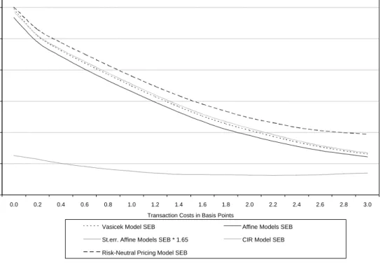
In figure 2A, we include a plot of the sensitivity of the SEBs to the size of transaction costs. For comparison, we also graph the SEB of the risk-neutral pricing model, that is obtained if in a one-factor affine model the market price of risk is equal to zero. Hence, the monthly SDF of this model is simply equal

(18)

to exp(&_r . The graph shows that the SEB for this simple model is always larger than the SEBs of all

1t)

other models, as could be expected. Still, the difference between the SEB of the risk-neutral pricing model and the SEBs of the other models is not very large. The graph also shows that, for the Vasicek, CIR and affine models, the size of the SEB is around 0.01 at transaction costs of 1.8 basis point, which is economically rather small. In the frictionless case, extreme short and long positions in T-bills and bonds blow up the differences between pricing errors of T-bills and bonds so that standard test procedures reject the affine models. We, however, show that, if small transaction costs are taken into account, these differences in pricing errors are not large enough to cause rejection of the models.

In figure 1, the t-ratios of the Vasicek SEB-multipliers indicate that, for transaction costs of 1 basis point, only the pricing errors of some individual assets contribute to the misspecification size of the one-factor models. In the absence of transaction costs, both the unconditional and the conditional 6-month and 9-month T-bill returns contribute most significantly to the size of the two-step SEB. At transaction costs of 1 basis point, none of the individual assets contributes significantly to the size of the SEB. In fact, for several bonds, the multipliers are exactly equal to zero; therefore, these assets do not contribute at all to the size of the SEB.

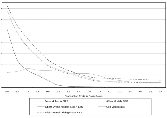
So far, all results discussed are based on the assumption that the holding period is equal to one month. To analyze the influence of this assumption, we now turn to the results of a quarterly holding period. In the lower panel of table 5 we give the p-values of the Wald-test and the SEBs of the one-factor models for a quarterly holding period, without transaction costs. Again, in all cases, the models are rejected statistically. If pricing errors and returns were independently and identically distributed over time, the SEB and its asymptotic standard error should increase approximately by a factor 3. From table 5 we see that this rule of thumb is not exactly true: we find an increase in the SEB that is a little smaller than 3.

For the case of transaction costs, the results for the quarterly holding period are given in the lower panel of table 8. Compared to the monthly holding period, larger transaction costs of 3.1 basis points are required to accept the models statistically and to obtain a small SEB. Because the monthly pricing errors are only very weakly correlated over time, the quarterly pricing errors are larger than the monthly pricing errors and, therefore, also larger transaction costs are required to accept the model statistically and to obtain a small SEB. The difference between the results for the monthly and quarterly SEBs is striking. It implies that the choice of holding period is a non-trivial one. Figure 2B shows that there is still a strong influence of small transaction costs on the SEBs, although it is clearly less strong than for monthly holding periods.

6.2 Two-Factor Affine Models

Next we present results for two-factor Vasicek, CIR and general affine models, again for the cases without and with transaction costs and monthly and quarterly holding periods. In table 9 we present the results for the Wald test and the SEB for the two-factor models, for both monthly and quarterly holding returns and

(19)

no transaction costs. The two-factor models are all rejected by the Wald-test, under the assumption of frictionless markets. The results also show that the SEBs of the Vasicek and CIR models do not decrease significantly compared to the one-factor case when we add the second factor, which is consistent with the high correlation between pricing errors of one-factor and two-factor Vasicek (and CIR) models reported in table 6. However, the SEB of the general two-factor affine model is much lower than the SEB of the one-factor affine model and the two-one-factor Vasicek and CIR models. Because there are many other two-one-factor affine models than the two-factor Vasicek and CIR models, this result indicates that there is a two-factor affine model, different from the two-factor Vasicek and CIR models, that has a much lower specification error. Still, under the assumption of frictionless markets, the general class of two-factor affine models is rejected by the Wald test.

These results are comparable to, for example, the results of Pearson and Sun (1994), who estimate a two-factor CIR model using ML based on two asset returns and who, subsequently, analyze the implications for all other T-bill and bond prices. They conclude that the two-factor CIR model cannot price all these assets correctly and reject this model statistically. In the previous section we have indicated how the presence of transaction costs can provide a possible explanation for the misspecification of the one-factor models in frictionless markets, whereas it thus seems that adding a second one-factor without transaction costs does not satisfactorily solve this misspecification.

On the basis of table 7, we find that the pricing errors of the one- and two-asset portfolios are roughly the same for the one- and two-factor Vasicek models, which is again consistent with the high correlation between the pricing errors of the one- and two-factor Vasicek models. This is also confirmed by figures 1 and 3 in which we find quite similar SEB-multipliers for both the one- and two-factor Vasicek models. For the case of transaction costs, the results are given in table 10 and in figures 4A-B. Qualitatively, the results are quite similar to the results for the one-factor models, although the transaction costs that are needed to accept the model, the so-called ‘critical transaction costs’, are a little smaller for the two-factor Vasicek and CIR models, namely 2.2 basis points for the quarterly holding period and the All Maturities Asset Set. For the general class of affine two-factor models and quarterly holding periods, transaction costs of around 2.8 basis points are needed to avoid rejection of the model, given our sample size and sample period. Figures 4A-B demonstrate again the strong sensitivity of the SEB to the size of transaction costs. These figures also show that the difference between the SEB of the general affine two-factor model and the SEBs of the Vasicek and CIR two-factor models does not disappear when transaction costs are included.

(20)

7 Summary and Conclusions

In this paper we analyze the bond pricing implications of affine interest rate models, allowing for the presence of transaction costs. The goal of the paper is to assess the importance of incorporating market frictions for tests of asset pricing models.

We test the models formally for different sizes of transaction costs, using a Wald-test, and we measure the size of misspecification of one- and two-factor affine interest rate models and analyze how sensitive the misspecification size is to the size of the transaction costs. Our analysis can be seen as an extension of Luttmer (1996), because we use the stronger specification error bound test, as opposed to the volatility bound that is used by Luttmer (1996), which is a special case of the specification error bound. Also, Luttmer (1996) focuses on consumption-based asset pricing models, whereas we analyze models for the term structure of interest rates.

We find that, under the assumption of frictionless markets, one-factor affine interest rate models misprice T-bill and bond returns in a significant way. Small differences in the pricing errors of highly correlated T-bill returns lead to a strong rejection of the one-factor models. Adding a second factor to the models does not explain the misspecification of one-factor models: two-factor models are also strongly rejected. We find, however, if we take transaction costs of about 1.5 basis points into account, that the misspecification of the one- and two-factor models disappears, in case of a monthly holding period. For quarterly holding periods, these models are not rejected at transaction costs of around 3 basis points.

(21)

v(2) / E[Y k t(2)xi,kt] E[q_i_,_t] ' 1, i'1,..,n, (A.1) ˆ v(2)_i / 1 Tj T t'1Ytk(2)xi,kt 1 Tj T t'1qi,t , i'1,...,n. _(A.2)

T( ˆv( ˆ2)&4) 6 N(0, (I&M₀)W(2₀) (I&M₀))), (A.3)

Appendix: The Limit Distribution of the All Affine Models

Wald Test

To obtain Wald-tests of general affine models, we estimate the parameters 2 in the SDF (10) by minimizing the test-statistic in (15), with J_s_'J_l_'1, over the parameters 2 as well. Subsequently, we substitute these parameter estimates in the SDF in (6), and test the (overidentifying) Euler restrictions, both in case of frictionless markets and in case of transaction costs, using the test-statistic in (15). The estimation strategy for 2 influences the limit distribution of the Wald-test in (15). In this appendix we derive this limit distribution. We will show that the limit distribution of this minimized test-statistic is still a mixture of chi-square distributions, but with less degrees of freedom than the test-statistic that is not minimized over the parameters 2.

The Euler restrictions used for estimation are of the form

where 2 is a q-dimensional parameter vector, with n>q. To simplify notation, we define the estimator of the left-hand side of (A.1) for a given value of 2 as follows

We then estimate the parameter 2 by applying GMM to the moment restrictions (A.1), with a consistent estimate for the optimal weighting matrix. This is equivalent to minimizing (15) over 2 with transaction costs set to zero. Denote the unique probability limit of the GMM-estimate with 2ˆ 2₀. The asymptotic covariance matrix of vˆ( ˆ2) is given by

where W(2₀) is the asymptotic covariance matrix of vˆ(2₀), and where M0 is given by (see Gourieroux and

(22)

>_w ' min_v_0ún T[ ˆv( ˆ2)&v])Wˆ( ˆ2)&1[ ˆv( ˆ2)&v] s.t. 1 Js # vi # 1 Jl, i'1,...,n. (A.5) Mv(2₀) M2) [ Mv(2₀)) M2 W(20)&1 Mv(2₀) M2) ] &1 Mv(20)) M2 W(20)&1. (A.4)

The covariance matrix in (A.3) has rank n-q. As noted by Gourieroux and Monfort (1995), a generalized inverse of the matrix (I&M₀)W(2₀) (I&M₀)) is given by W(2₀)&1, so that we can consistently estimate this generalized inverse by Wˆ( ˆ2)&1, which consists of replacing population moments with sample moments in the asymptotic covariance matrix.

In a second step, the test-statistic is obtained from the following minimization

Then, conditional on the event that all restrictions are estimated to be binding in (A.5), the statistic in (A.5) is asymptotically P2_n_&_q-distributed under the null hypothesis. Similarly, conditional on the event that exactly p restrictions in (A.5) are estimated to be binding, the distribution of the test-statistic under the null hypothesis is P2_max(_p_&_q_,0), where P2₀ is the unit mass at the origin. The probability weights for each of these events can be found using the degenerated multivariate normal limit distribution of vˆ( ˆ2) under the null hypothesis given in equation (A.3). Hence, the limit distribution of the test-statistic (A.5) under the null hypothesis is a mixture of chi-square distributions with degrees of freedom between 0 and n-q.

(23)

References

Babbs, S.H., and K.B. Nowman (1999), ‘Kalman Filtering of Generalized Vasicek Term Structure Models’, Journal of Financial and Quantitative Analysis, 34, 115-130.

Backus, D.K., S. Foresi, A. Mozumdar, and L. Wu (1997), ‘Predictable Changes in Yields and Forward Rates’, Working Paper New York University and NBER.

Backus, D.K., and S.E. Zin (1994), ‘Reverse Engineering the Yield Curve’, Working Paper NBER.

Bansal, R. (1997), ‘An Exploration of the Forward Premium Puzzle in Currency Markets’, Review of Financial Studies, 10, 131-166.

Brown, R.H., and S.M. Schaefer (1994), ‘The Term Structure of Real Interest Rates and the CIR Model’, Journal of Financial Economics, 35, 3-42.

Campbell, J.Y., A. Lo, and A. MacKinley (1997), ‘The Econometrics of Financial Markets’, Princeton University Press.

Chen, R. and L. Scott (1993), ‘ML Estimation for a Multi-Factor Equilibrium Model of the Term Structure’, Journal of Fixed Income, December.

Cochrane, J.H. (1996), ‘A Cross-sectional Test of an Investment-based Asset Pricing Model’, Journal of Political Economy, 104, 572-621.

Cox, J., J. Ingersoll and S. Ross (1985), ‘A Theory of the Term Structure of Interest Rates’, Econometrica 53, 385-408.

Dai, Q., and K.J. Singleton (1997), ‘Specification Analysis of Affine Term Structure Models’, Working Paper, Stanford University.

De Jong, F. (1999), ‘Time-series and Cross-section Information in Affine Term Structure Models’, CEPR Discussion Paper.

(24)

Duffie, D.J., and R. Kan (1996), ‘A Yield-factor Model of Interest Rates’, Mathematical Finance, 6, 379-406.

Ferson, W.E., and A.F. Siegel (1998), ‘Optimal Moment Restrictions on Stochastic Discount Factors’, Working Paper, University of Washington.

Gibbons, M.R., and K. Ramaswamy (1993), ‘A Test of the CIR Model of the Term Structure’, Review of Financial Studies, 6, 619-658.

Gourieroux, C., and A. Monfort (1995), Statistics and Econometric Models, Cambridge University Press.

Hansen, L.P. (1982), ‘Large Sample Properties of Generalized Methods of Moments Estimators’, Econometrica, 50, 1029-1054.

Hansen, L.P., and R. Jagannathan (1991), ‘Implications of Security Market Data for Models of Dynamic Economies’, Journal of Political Economy, 99, 225-262.

Hansen, L.P., and R. Jagannathan (1997), ‘Assessing Specification Errors in Stochastic Discount Factor Models’, Journal of Finance, 52, 557-590.

Hansen, L.P., J.C. Heaton, and E. Luttmer (1995), ‘Econometric Evaluation of Asset Pricing Models’, Review of Financial Studies, 8, 237-274.

He, H., and D.M. Modest (1995), ‘Market Frictions and Consumption-Based Asset Pricing’, Journal of Political Economy, 101, 94-117.

Jouini, E., and H. Kalal (1995), ‘Martingales, Arbitrage and Securities Markets with Transaction Costs’, Journal of Economic Theory, 66, 178-197.

Kan, R. and G. Zhou (1999), ‘A Critique of the Stochastic Discount Factor Methodology’, Journal of Finance, forthcoming.

Kodde, D.A., and F.C. Palm (1986), ‘Wald Criteria for Jointly Testing Equality and Inequality Restrictions’, Econometrica, 54, 1243-1248.

(25)

Newey, W.K., and K.D. West (1987), ‘A Simple, Positive Semi-Definite, Heteroskedasticity and Autocorrelation Consistent Covariance Matrix’, Econometrica, 55, 703-708.

Pearson, N.D., and T.S. Sun (1994), ‘Exploiting the Conditional Density in Estimating the Term Structure: an Application of the CIR model’, Journal of Finance, 49, 1279-1304.

Prisman, E. (1986), ‘Valuation of Risky Assets in Arbitrage Free Economies with Frictions’, Journal of Finance, 41, 545-560.

Snow, K.N. (1991), ‘Diagnosing Asset Pricing Models Using the Distribution of Asset Returns’, Journal of Finance, 46, 955-983.

Stambaugh, R. (1988), ‘The Information in Forward Rates’, Journal of Financial Economics, 21, 41-70.

Sun, T.S. (1992), ‘Real and Nominal Interest Rates: A Discrete-time Model and its Continuous Time Limit’, Review of Financial Studies, 5, 581-611.

Vasicek, O. (1977), ‘An Equilibrium Characterization of the Term Structure’, Journal of Financial Economics, 5, 177-188.

Vuong, Q. (1989), ‘Likelihood Ratio Tests for Model Selection and Non-nested Hypotheses’, Econometrica, 57, 307-333.

Wolak, F.A. (1989), ‘Local and Global Testing of Linear and Nonlinear Inequality Constraints in Nonlinear Econometric Models’, Econometric Theory, 5, 1-35.

Wolak, F.A. (1991), ‘The Local Nature of Hypothesis Tests Involving Inequality Constraints in Nonlinear Models’, Econometrica, 59, 981-995.

(26)

Tables

Table 1. Properties of Interest Rates.

The sample moments are calculated using the CRSP Fama Files, which contains monthly data for the period 1972-1997. Interest rates are expressed on a yearly basis.

Maturity in Months Mean St. Deviation Autocorrelation

1 6.61% 2.67% 0.96 3 7.03% 2.78% 0.97 12 7.50% 2.64% 0.97 24 7.78% 2.49% 0.98 36 7.96% 2.38% 0.98 48 8.11% 2.30% 0.98 60 8.20% 2.24% 0.98

Table 2. Properties of Holding Returns.

The table contains sample moments of monthly holding returns on T-bills with maturities of 1, 3 ,6 and 9 months and monthly holding returns on portfolios of bonds with maturities in a certain interval, which are calculated using CRSP data for 1972-1997.

Maturity in Months Mean St. Deviation Autocorrelation

1 0.56% 0.23% 0.95 3 0.61% 0.27% 0.81 6 0.63% 0.36% 0.50 9 0.65% 0.49% 0.36 24-36 0.69% 1.20% 0.17 48-60 0.70% 1.67% 0.15 60-120 0.73% 2.07% 0.14 > 120 0.78% 2.92% 0.12

(27)

Table 3. Bid-Ask Spreads of T-bill Prices.

Bid-ask spreads are in basis points and calculated by dividing the difference between bid and ask prices by the mid price. Data on bid and ask prices come from the CRSP T-bill dataset.

Maturity Average Bid-Ask Spread, 1972-1997. Standard Deviation, 1972-1997. Average Bid-Ask Spread, 1987-1997. Standard Deviation, 1987-1997. 1 month 1.3 bp 1.4 bp 0.4 bp 0.3 bp 3 months 2.1 bp 2.1 bp 0.5 bp 0.2 bp 6 months 4.1 bp 4.0 bp 1.1 bp 0.2 bp 9 months 5.9 bp 5.3 bp 1.6 bp 0.3 bp

Table 4. GMM Estimation Results: Vasicek and CIR Models.

The table contains the results of GMM estimation of the discrete-time, monthly, one-factor and two-factor Vasicek and CIR models, based on 12 moment conditions, using the optimal weighting matrix. In square brackets the t-ratios are given, which have been calculated using the Newey-West method with 12 lags. Also presented are the mean and variance of the implied stochastic discount factor, and the GMM J-statistic. All parameters are expressed on a monthly basis.

Parameter 1-Factor Vasicek 2-Factor Vasicek 1-Factor CIR 2-Factor CIR µ1 0.0095 [5.9] 0.027 [1.8] 0.0084 [8.7] 0.0015 [0.9] 100 $1 0.031 [3.2] 0.022 [1.1] - -"11 - - 0.0064 [7.6] 0.012 [3.7] 1-711 0.012 [4.4] 0.004 [0.8] 0.016 [5.2] 0.012 [2.2] (1 -256.94 [-2.9] -356.63 [-0.6] -126.19 [-5.5] -106.13 [-3.0] µ2 - - - 0.023 [4.1] 100 $2 - 0.061 [3.1] - -"22 - - - 0.020 [7.0] 1-722 - 0.106 [0.8] - 0.138 [4.2] (2 - -351.42 [-2.6] - -61.62 [-8.7] Mean of SDF 0.9945 0.9933 0.9981 0.9932 St.Dev. of SDF 0.0887 0.2108 0.1003 0.1754 J-Statistic (p-value) 21.71 [0.006] 10.68 [0.06] 21.17 [0.007] 7.44 [0.11]

(28)

Table 5.Wald-test and SEB for One-Factor Models in Frictionless Markets.

The table reports Wald test results and the SEB for the one-factor affine models and monthly and quarterly investment horizons. Asymptotic standard errors of the SEB are given in brackets. To calculate the asymptotic covariance matrices for the quarterly holding period, we use the Newey-West method with 2 lags to correct for the overlapping nature of the returns.

Asset set Vasicek Model CIR Model All Affine Models

Monthly holding period

Wald p-value: Short-maturities 0.000 0.000 0.000

Wald p-value: Long-maturities 0.041 0.015 0.000

Wald p-value: All-maturities 0.000 0.000 0.000

SEB: Short-maturities 0.619 (0.096) 0.625 (0.104) 0.575 (0.100)

SEB: Long-maturities 0.215 (0.055) 0.206 (0.052) 0.181 (0.055)

SEB: All-maturities 0.688 (0.109) 0.694 (0.120) 0.651 (0.106)

Quarterly holding period

Table 6. Pricing Error Correlations across Models.

For each asset in the all maturities asset-set, the correlation between the pricing errors of two models is calculated. The table presents the average of these correlations over all assets. For the general affine models, the pricing errors that result from the minimization of the SEB in (21) are used.

1F Vasicek 1F CIR 1F Affine 2F Vasicek 2F CIR 2F Affine

1F Vasicek 1 1F CIR 0.998 1 1F Affine 0.723 0.728 1 2F Vasicek 0.961 0.953 0.649 1 2F CIR 0.68 0.695 0.28 0.718 1 2F Affine 0.001 0.005 0.336 0.087 -0.087 1

(29)

Table 7. Normalized Pricing Errors of Long-Short Portfolios:

One- and Two-Factor Vasicek Models.

The table contains monthly pricing errors for one- and two-asset portfolios. For each T-bill, the long-short portfolio refers to a portfolio of the particular T-bill and the 1-month T-bill. For each bond, the long-short portfolio refers to a portfolio in the particular bond and the 2-3 year maturity bond. For these long-short portfolios, the multiplier-vector or weight-vector 8 in (19) always contains a positive and an equally large negative element. The portfolio weights are normalized as in equation (19). In brackets, standard errors of the pricing errors are presented.

1-Factor Vasicek 1-Factor Vasicek 2-Factor Vasicek 2-Factor Vasicek Unconditional Returns Normalized Pricing Error Individual Assets Normalized Pricing Error Long-Short Portfolios Normalized Pricing Error Individual Assets Normalized Pricing Error Long-Short Portfolios T-bill 1-month 0.0076 (0.0085) - 0.0084 (0.0122) -T-bill 3-months 0.0080 (0.0085) 0.354 (0.052) 0.0087 (0.0122) 0.302 (0.056) T-bill 6-months 0.0080 (0.0084) 0.148 (0.056) 0.0086 (0.0120) 0.090 (0.060) T-bill 9-months 0.0080 (0.0083) 0.100 (0.057) 0.0085 (0.0119) 0.046 (0.061) Bond 2-3 years 0.0078 (0.0078) - 0.0079 (0.0113) -Bond 4-5 years 0.0075 (0.0075) 0.039 (0.057) 0.0076 (0.0110) 0.063 (0.060) Bond 5-10 years 0.0076 (0.0073) 0.016 (0.053) 0.0075 (0.0107) 0.041 (0.060) Bond >10 years 0.0077 (0.0070) 0.009 (0.031) 0.0074 (0.0103) 0.029 (0.057) Conditional Returns T-bill 1-month 0.0065 (0.0077) - 0.0003 (0.0098) -T-bill 3-months 0.0069 (0.0077) 0.415 (0.052) 0.0004 (0.0097) 0.365 (0.056) T-bill 6-months 0.0069 (0.0076) 0.199 (0.056) 0.0004 (0.0096) 0.143 (0.061) T-bill 9-months 0.0070 (0.0075) 0.145 (0.058) 0.0004 (0.0095) 0.091 (0.064) Bond 2-3 years 0.0070 (0.0070) - 0.0006 (0.0090) -Bond 4-5 years 0.0070 (0.0068) 0.011 (0.046) 0.0008 (0.0089) 0.029 (0.059) Bond 5-10 years 0.0072 (0.0066) 0.020 (0.053) 0.0007 (0.0087) 0.003 (0.057) Bond >10 years 0.0075 (0.0063) 0.029 (0.054) 0.0005 (0.0085) 0.008 (0.056)

(30)

Table 8. Critical Transaction Costs for One-Factor Models.

The critical transaction costs are defined as the amount of transaction costs for which the Wald p-value is equal to 0.05. Transaction costs are relative to the price and presented in basis points.The table presents results are for monthly and quarterly holding periods.

Short-maturities 0.9 bp 0.9 bp 0.8 bp

Long-maturities 0.1 bp 0.1 bp 0.1 bp

All-maturities 1.0 bp 0.9 bp 0.8 bp

Table 9.Wald-test and SEB for Two-Factor Models in Frictionless Markets.

The table reports Wald test results and the SEB for the two-factor affine models. Asymptotic standard errors of the SEB are given in brackets. To calculate the asymptotic covariance matrices for the quarterly holding period, we use the Newey-West method with 2 lags to correct for the overlapping nature of the returns.

Monthly Holding Period

(31)

Table 10. Critical Transaction Costs for Two-Factor Models.

The critical transaction costs are defined as the amount of transaction costs for which the Wald p-value is equal to 0.05. Transaction costs are relative to the price and presented in basis points.The table presents results are for monthly and quarterly holding periods.

(32)

Figure 1. SEB-Multipliers One-Factor Vasicek Model. T-ratios of SEB-multipliers for monthly returns and one-factor Vasicek model, at transaction costs of 0 and 1 basis point.

-4 -3 -2 -1 0 1 2 3 1 3 6 9 ₃₀ ₅₄ ₉₀ 120

1-Cond 3-Cond 6-Cond 9-Cond30-Cond54-Cond90-Cond_120-Cond

Maturity in Months T-Ratio Monthly 1-Factor Vasicek: No Trans. Costs. Monthly 1-Factor Vasicek: 1 bp Trans. Costs.

Figure 2A. Monthly SEB for One-Factor Models. The graph shows the SEB for different sizes of

transaction costs, for the risk-neutral pricing model, and one-factor Vasicek, CIR and affine models. Monthly holding periods.

0 0.1 0.2 0.3 0.4 0.5 0.6 0.7 0.0 0.2 0.4 0.6 0.8 1.0 1.2 1.4 1.6 1.8 2.0 2.2 2.4 2.6 2.8 3.0 Transaction Costs in Basis Points

SEB

Vasicek Model SEB Affine Models SEB St.err. Affine Models SEB * 1.65 CIR Model SEB Risk-Neutral Pricing Model SEB