Modified balanced random forest for improving
imbalanced data prediction
Zahra Putri Agusta a,1,*, Adiwijaya b,2
a Human Computer Interaction Department, Surya University, Tangerang, Indonesia b School of Computing, Telkom University, Bandung, Indonesia
1[email protected]; 2 [email protected] * corresponding author
1.
Introduction
Random Forest is a machine learning classification algorithm that has been proven to perform well in conducting classification compared to other classification algorithms [1]. The algorithm is easy to implement and produces a model with better performance [2][3]. Random Forest has shown higher performance compared to five other classification algorithms, such as KNN, Naïve-Bayes, C4.5, AdaBoost, and ANN [4]. However, imbalanced data poses a big challenge for Random Forest techniques
[5]. Classifying imbalanced data can decrease the effectiveness of classification techniques, since the classification process always assumes that the data is drawn from the same distribution as the training data and at the same misclassification cost. Therefore, a process for handling imbalanced data for the classification algorithm is required [6][7].
Several studies have addressed the issue of imbalanced data. For example, Wu et al. [8] used the Random Forest algorithm in an insurance business problem, where the insurance data had characteristics of class imbalance. The data was analyzed using undersampling with a KKN algorithm approach. The technique reduced the data learning process for the Random Forest. Khalilia et al. [9] used Random sub-sampling to handle imbalanced data in predicting disease risk. First, imbalanced medical data was treated, where the training data was divided into multi-sampling data. It was also ensured that each sub-sample data was balanced between the minority and majority. The final result showed that the Random Forest algorithm, which had applied imbalanced data treatment beforehand, produced superior performance compared to the SVM classification algorithm. One study conducted a data handling A R T I C L E I N F O A B S T R A C T
Article history Received July 25, 2018 Revised December 5, 2018 Accepted December 19, 2018 Available online March 26, 2019
This paper proposes a Modified Balanced Random Forest (MBRF) algorithm as a classification technique to address imbalanced data. The MBRF process changes the process in a Balanced Random Forest by applying an under-sampling strategy based on clustering techniques for each data bootstrap decision tree in the Random Forest algorithm. To find the optimal performance of our proposed method compared with four clustering techniques, like: K-MEANS, Spectral Clustering, Agglomerative Clustering, and Ward Hierarchical Clustering. The experimental result show the Ward Hierarchical Clustering Technique achieved optimal performance, also the proposed MBRF method yielded better performance compared to the Balanced Random Forest (BRF) and Random Forest (RF) algorithms, with a sensitivity value or true positive rate (TPR) of 93.42%, a specificity or true negative rate (TNR) of 93.60%, and the best AUC accuracy value of 93.51%. Moreover, MBRF also reduced process running time.
This is an open access article under the CC–BY-SA license.
Keywords Imbalanced Data Random Forest Algorithm Balanced Random Forest Customer Churn Classification Technique
technique by combining two sampling data techniques, namely undersampling and SMOTE, to handle the imbalanced data problem in a weighted Random Forest [10]. Another study carried out a combination of RUSBoost and Information Gain as the preprocessing method for churn prediction of imbalanced data [11]. However, some of the above researches handled imbalanced data such that the data handling process would still be in preprocessing before the classification algorithm is executed. Therefore, the direct effect of handling balanced data in the Random Forest algorithm could not be fully observed.
In this research, we discuss methods for handling imbalanced data based on the Random Forest and Balanced Random Forest (BRF) algorithms. The BRF puts imbalanced data handling into an algorithm process [12]. The BRFimplements an undersampling technique for every process of decision tree formation in the Random Forest algorithm, and therefore is known as the Balanced Random Forest, as it combines a sampling technique with an ensemble idea. However, BRF has a few weaknesses. The random undersampling process reveals wasted important data which could affect the classification result. Therefore, in this paper, we proposed a new approach, namely the Modified Balanced Random Forest (MBRF) algorithm. The method may not only improves accuracy but also reduces time complexity. This method changes the process of the Balanced Random Forest algorithm, which discard the majority of the data. In other words, the random undersampling of BRF is replaced by a clustering technique. The technique of training data distribution is also adjusted to the number of used random forest parameters. To get the optimal method, we compared four clustering techniques namely K-MEANS, Spectral clustering, Agglomerative clustering, and Ward Hierarchical clustering [13] - [18]. These four clustering techniques use a defined the number as the base of clusters. The number of clusters in MBRF method will be input according to the number of minority classes.
2.
Method
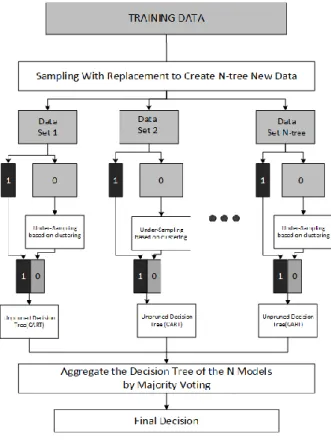
In this study, MBRF (Fig. 1) is proposed to improve the prediction performance of the Random Forest and Balanced Random Forest algorithms. We proposed changes in the process of Balanced Random Forest by taking advantage of other algorithms, namely clustering algorithms.
This method begins with taking data from the training data (D). The data will be split as many as the input of N tree, which becomes Di (D1, D2, D3, until Dntree). Each Di has (Xi and Yi), where Xi is the vector data and Yi is the class label. After that, the Balanced Random Forest algorithm is run in which the data is split into two bootstrap rows, Di+, Di− (the class labeled “+” is churn data and the class labeled “−” is non-churn data). To form the tree, the two bootstrap rows will be used, in which each bootstrap takes the same total data to that of the data in the minority class. Then, undersampling is conducted on the majority data using a clustering technique, in which the centroids in each cluster will be input into the bootstrap, and the total number of clusters will be the same as the total minority data. In this way, a centroid with the same total as that of the minority class will be produced.
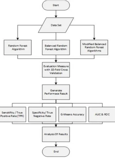
Balanced Random Forest is said to be a process that combines undersampling majority classes and ensemble learning ideas [19]. In the method we propose, under-sampling majority is conducted based on clustering, so undersampling data for building a tree can represent all data, where clustering data will be made into a cluster. Therefore, similar data will be combined such that there will be no data that is not used from down sampling. It also helps to remove the weakness of the undersampling technique, in which there are often various important rows, which are not mentioned in the Random Forest learning process [11]. It is better if every tree formed in the Forest does not have any relationship or high correlation with other trees. Hence, a random process is conducted during classification of bootstrap rows, where the total bootstrap will be equal to the total N-tree. The design process for this research is described in Fig. 2.
Fig. 2. Research Design Flowchart 2.1.Data set
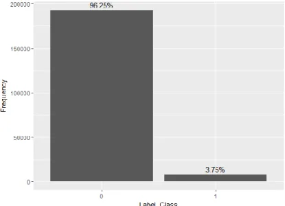
This study used customer churn data obtained from PT Telkom Indonesia. The data amounted to 200387 row data, which consisted of 192863 row non-customer churn data and 7524 row customer
churn data. Hence, the churn rate is 3.75%, resulting in imbalanced data and 52 attributes in the data (Fig. 3).
Fig. 3. Distribution of non-churn rows (Label_Class: 0) and churn rows (Label_Class: 1) in the Dataset 2.2.Evaluation Measure
In this study, we used sensitivity, specificity, ROC Curve, and AUC to assess the prediction models, have been used per several researcher for classifier assessment over imbalanced data set, as the publication of [20]-[22]. Sensitivity and specificity of the effectiveness of an algorithm in one class can be divided into positive and negative, respectively [23]. Based on our case, churn prediction aims to predict the true positive class, so that the higher the sensitivity or true positive rate, the better the prediction of customer churn [24].
Besides sensitivity and specificity, calculation of model accuracy using G-means was also performed for both classes (positive and negative) [23]. This is different from the calculation of general accuracy, which cannot be used for imbalanced data because it has more weight in the majority class (negative) than the minority class (positive). This makes it difficult for the classifier to show in a minority class (negative) [23]. Therefore, if the model wrongly classified the minority class, the accuracy would still be high [25], whereas G-means would give a more realistic result. G-means measurement avoids inclination towards the majority class (negative class) [26].
Other evaluations used are ROC (Receiver Operating Characteristics) and AUC (Area Under ROC Curve). The benefit of using the ROC curve is that we can easily determine the model with the best performance [27]. Meanwhile, AUC is the area under the ROC curve. AUC summarizes the ROC curve performance into one quantity value. The AUC value is about 0.5–1,where the bigger the AUC value, the better the model [23]. Before performing the model evaluation calculation, we first calculated the total true positive (TP), true negative (TN), false positive (FP) (actual negative but it is predicted positive), and false negative (FN) (actual positive but it is predicted negative) values [28][29].
3.
Results and Discussion
This research purposes maintaining imbalance data technique by using MBRF (Modified Balance Random Forest). To examine and find out improvement of proposed model, they are compared with random forest algorithm and Balanced Random Forest (BRF) algorithm. To obtain optimal parameter, we try 10 input parameters of total of tree (5,10 ,15 ,20 ,25 ,50 ,60, 70 ,90 ,100). After doing running process with 10 parameters, it is obtained optimal parameter in total of 10 trees. However, the result is not giving significant difference toward parameter of other tree. It is because random forest parameter is insensitive. Even though it does not affect the accuracy but this parameter does affect toward the time, in which the higher parameter of random forest, the longer time is needed. To avoid over fitting
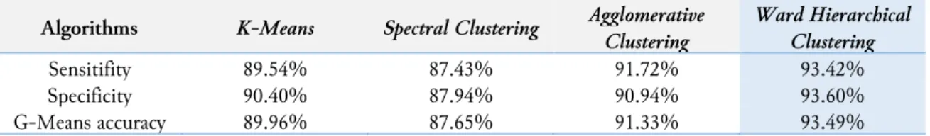
problem, we obtained the performance measure using 10-fold cross validation which uses of data as for training the algorithm and the remaining for testing purpose and repeats the process 10 times [30]. To see the optimal performance of the clustering techniques, we compared the four techniques mentioned earlier. The comparison is conducted using the same N-tree and K-fold input (n-tree = 10 and 10-fold) in the majority class data in each decision tree in the same random forest. Table 1 shows the result of the performance measurement.
Table 1. Experiment results on each Algorithms Clustering
Algorithms K-Means Spectral Clustering Agglomerative
Clustering Ward Hierarchical Clustering Sensitifity 89.54% 87.43% 91.72% 93.42% Specificity 90.40% 87.94% 90.94% 93.60% G-Means accuracy 89.96% 87.65% 91.33% 93.49%
Ward Hierarchical Clustering provides better performance than other clustering techniques. However, it is significantly different withthe Agglomerative Clustering technique. This is because these two clustering techniques have large scalability so that they can provide a large number of cluster inputs with large amounts of data. Unlike the K-Means which has a limited number of clusters eventhough it can work with large data. Among the 4 techniques of clustering, Spectral Clustering provides low performance because it is not optimal for large data and large number of clusters. Therefore, in MBRF the clustering technique used is Ward Hierarchical Clustering. Table 2 shows a comparison of the performance results when MBRF is compared to RF and BRF.
Table 2. Experiment results on each method
Evaluation Measure Random Forest
(RF) BalancedRandom Forest (BRF) Modified Balanced Random Forest (MBRF) Sensitifity 57.20% 75.93% 93.42% Specificity 99.12% 99.12% 93.60% G-Means 75.16% 86.75% 93.49% AUC 78.16% 87.52% 93.51%
Running time 435.50 Sec 80. 47Sec 57.80Sec
We compared the classification results of the Random Forest, Balanced Random Forest and Modified Balanced Random Forest. To avoid over fitting problem, we obtained the performance using 10-fold cross validation which uses 9/10 of data as for training the algorithm and the remaining for testing purpose and repeats the process 10 times.
From the Table 2 produced better value than other two methods which are Random forest without balance, Balanced Random Forest without modified balance random forest, in which G-means value has the value of 0.9349 or 93.49%, and so AUC 0.9351 or 93.51%. In the case of churn prediction, it has goal in which model has better specificity value. MBRF and BRF result recall value or sensitivity which are better than RF. It is because two methods conduct data balance in forming tree. MBRF results running time better than other algorithm, so that overall MBRF gives improvement of churn prediction and better effectiveness of running time.
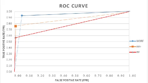
In Fig. 4, the ROC Curve was used to compare the performance of the three methods. The ROC curve consists of x (TPR) and y (1-TNR), in which the point in the curve that forms a line is based on conducting tree tests based on this curve. MBRF, which is marked in yellow, has an AUC value of 1 (bigger under curve area and approach), proving that the proposed MBRF algorithm is better than the BRF and RF algorithms. The ROC curve can be used to determine which method is best [27].
The tree parameters did not give a significant effect on the result because these could be observed as a point. This means that the AUC value is not too different (almost the same), so the parameter in this method is insensitive towards the result. However, it really affected execution time. Random Forest resulted in the longest running time, with 25 trees resulting in 621 seconds or 10 minutes. Meanwhile, the shortest running time was MBRF with 25 trees in 39.01 seconds.
Fig. 4. Comparison of ROC Curves between RF, BRF, and MBRF
4.
Conclusion
A method called the Modified Balanced Random Forest (MBRF) has been proposed. The proposed technique provides low precision between the accuracy of classifying majority classes and minority classes, produce almost the same sensitivity (TPR) and Specificity (TNR). Moreover, the new model has able to reduce the processing time. The used Random Forest parameter, did not give different result in each model due to its insensitivity. However, these parameters affect the running time as the increase of the time to form the trees. This method is inefficient for a small sample data. A future research should be conducted to overcome the weakness of MBRF.
References
[1] S. Singh and P. Gupta, “Comparative study ID3, cart and C4 . 5 Decision tree algorithm: a survey,” Int. J.
Adv. Inf. Sci. Technol., 2014, doi: 10.15693/ijaist/2014.v3i7.47-52.
[2] L. Breiman, “Random forests,” Mach. Learn., vol. 45, no. 1, pp. 5-32, 2001, doi: 10.1023/A:1010933404324. [3] H. Aydadenta and Adiwijaya, “A Clustering Approach for Feature Selection in Microarray Data Classification Using Random Forest,” J. Inf. Process. Syst., vol. 14, no. 5, pp. 1167–1175, 2018, doi:
10.3745/JIPS.04.0087.
[4] G. Esteves and J. Mendes-Moreira, “Churn perdiction in the telecom business,” in 2016 11th International
Conference on Digital Information Management, ICDIM 2016, 2016, doi: 10.1109/ICDIM.2016.7829775.
[5] A. Sonak and R. A. Patankar, “A Survey on Methods to Handle Imbalance Dataset,” Int. J. Comput. Sci.
Mob. Comput., vol. 4, no. 11, pp. 338–343, 2015, available at : Google Scholar.
[6] A. Ali, S. M. Shamsuddin, and A. L. Ralescu, “Classification with class imbalance problem: A review,” Int.
J. Adv. Soft Comput. its Appl., vol. 7, no. 3, pp. 176-203, 2015, available at: http://home.ijasca.com/data/
documents/13IJASCA-070301_Pg176-204_Classification-with-class-imbalance-problem_A-Review.pdf . [7] S. Du, F. Zhang, and X. Zhang, “Semantic classification of urban buildings combining VHR image and GIS
data: An improved random forest approach,” ISPRS J. Photogramm. Remote Sens., 2015, doi:
[8] Z. Wu, W. Lin, Z. Zhang, A. Wen, and L. Lin, “An Ensemble Random Forest Algorithm for Insurance Big Data Analysis,” in Proceedings - 2017 IEEE International Conference on Computational Science and Engineering and IEEE/IFIP International Conference on Embedded and Ubiquitous Computing, CSE and EUC
2017, 2017, doi: 10.1109/CSE-EUC.2017.99.
[9] M. Khalilia, S. Chakraborty, and M. Popescu, “Predicting disease risks from highly imbalanced data using random forest,” BMC Med. Inform. Decis. Mak., 2011, doi: 10.1186/1472-6947-11-51.
[10] V. Effendy and Z. K. a. Baizal, “Handling imbalanced data in customer churn prediction using combined sampling and weighted random forest,” 2014 2nd Int. Conf. Inf. Commun. Technol., 2014, doi:
10.1109/ICoICT.2014.6914086.
[11] E. Dwiyanti, Adiwijaya, and A. Ardiyanti, “Handling imbalanced data in churn prediction using RUSBoost and feature selection (Case study: PT. Telekomunikasi Indonesia regional 7),” in Advances in Intelligent
Systems and Computing, 2017, doi: 10.1007/978-3-319-51281-5_38.
[12] Ł. Kobyliński and A. Przepiórkowski, “Definition extraction with balanced random forests,” in Lecture Notes in Computer Science (including subseries Lecture Notes in Artificial Intelligence and Lecture Notes in
Bioinformatics), 2008, doi: 10.1007/978-3-540-85287-2_23.
[13] S. Ghosh and S. Kumar, “Comparative Analysis of K-Means and Fuzzy C-Means Algorithms,” Int. J. Adv.
Comput. Sci. Appl., 2013, doi: 10.14569/IJACSA.2013.040406.
[14] S. Venkateswara and V. Swamy, “A Survey : Spectral Clustering Applications and its Enhancements,” Int.
J. Comput. Sci. Inf. Technol., vol. 6, no. 1, pp. 185–189, 2015, available at: Google Scholar.
[15] A. Y. Shelestov, “Using the agglomerative method of hierarchical clustering as a data mining tool in capital market,” Int. J. "Information Theor. Appl., vol. 15, no. 1, pp. 382–386, 2018, available at:
http://hdl.handle.net/10525/80.
[16] K. Sasirekha and P. Baby, “Agglomerative Hierarchical Clustering Algorithm-A Review,” Int. J. Sci. Res.
Publ., 2013, doi: 10.1016/S0090-3019(03)00579-2.
[17] W. Tian, Y. Zheng, R. Yang, S. Ji, and J. Wang, “A Survey on Clustering based Meteorological Data Mining,” Int. J. Grid Distrib. Comput., vol. 7, no. 6, pp. 229–240, 2014, available at: Google Scholar. [18] A. Chowdhary, “Community Detection:Hierarchical clustering Algorithms,” Int. J. Creat. Res. Thoughts,
vol. 5, no. 4, pp. 2320–2882, 2017, available at: http://ijcrt.org/papers/IJCRT1704418.pdf.
[19] C. Chen, A. Liaw, and L. Breiman, “Using random forest to learn imbalanced data,” Univ. California,
Berkeley, 2004, available at: https://statistics.berkeley.edu/sites/default/files/tech-reports/666.pdf.
[20] D. Ramyachitra and P. Manikandan, “Imbalanced Dataset Classification and Solutions: a Review,” Int. J.
Comput. Bus. Res., vol. 5, no. 4, 2014, available at: http://www.researchmanuscripts.com/July2014/2.pdf.
[21] S. Sardari, M. Eftekhari, and F. Afsari, “Hesitant fuzzy decision tree approach for highly imbalanced data classification,” Appl. Soft Comput. J., 2017, doi: 10.1016/j.asoc.2017.08.052.
[22] E. AT, A. M, A.-M. F, and S. M, “Classification of Imbalance Data using Tomek Link (T-Link) Combined with Random Under-sampling (RUS) as a Data Reduction Method,” Glob. J. Technol. Optim., 2018, doi:
10.4172/2229-8711.s1111.
[23] M. Bekkar, H. K. Djemaa, and T. A. Alitouche, “Evaluation measures for models assessment over imbalanced data sets,” J. Inf. Eng. Appl., vol. 3, no. 10, pp. 27-38, 2013, available at: Google Scholar. [24] C. G. Weng and J. Poon, “A new evaluation measure for imbalanced datasets,” Proceedings of the 7th
Australasian Data Mining Conference., vol. 87, no. 6, pp. 27-32, 2008, available at:
http://dl.acm.org/citation.cfm?id=2449288.2449295.
[25] J. S. Akosa, “Predictive Accuracy : A Misleading Performance Measure for Highly Imbalanced Data,” SAS
Glob. Forum, 2017, available at: Google Scholar.
[26] Y. Zhang and D. Wang, “A Cost-Sensitive Ensemble Method for Class-Imbalanced Datasets,” Abstr. Appl.
Anal., 2013, doi: 10.1155/2013/196256.
[27] T. Fawcett, “An introduction to ROC analysis,” Pattern Recognit. Lett., 2006, doi:
[28] H. M and S. M.N, “A Review on Evaluation Metrics for Data Classification Evaluations,” Int. J. Data Min.
Knowl. Manag. Process, 2015, doi: 10.5121/ijdkp.2015.5201.
[29] A. K. Santra and C. J. Christy, “Genetic Algorithm and Confusion Matrix for Document Clustering,” IJCSI
Int. J. Comput. Sci. Issues, 2012, available at: Google Scholar.
[30] J. Pohjankukka, T. Pahikkala, P. Nevalainen, and J. Heikkonen, “Estimating the prediction performance of spatial models via spatial k-fold cross validation,” Int. J. Geogr. Inf. Sci., 2017, doi: