Clustering
Andrea Gaunersdorfer1and Cars Hommes2
1 Department of Business Studies, University of Vienna.
2 Center for Nonlinear Dynamics in Economics and Finance, University of
forthcoming in:
G. Teyssi`ere and A. Kirman (eds.), Long Memory in Eco-nomics, Springer-Verlag, 2005.Summary.
A simple nonlinear structural model of endogenous belief heterogeneity is proposed. News about fundamentals is an IID random process, but nevertheless volatility clustering occurs as an endogenous phenomenon caused by the interaction between different types of traders, fundamentalists and technical analysts. The belief types are driven by adaptive, evolutionary dynamics according to the success of the prediction strategies as measured by accumulated realized profits, conditioned upon price deviations from the rational expectations fundamental price. Asset prices switch irregularly between two different regimes — periods of small price fluctuations and periods of large price changes triggered by random news and reinforced by technical trading — thus, creating time varying volatility similar to that observed in real financial data.?Earlier versions of this paper were presented at the 27th annual meeting of the
EFA, August 23—26, 2000, London Business School, the International Workshop on Financial Statistics, July 5—8, 1999, University of Hong Kong, the Workshop on Expectational and Learning Dynamics in Financial Markets, University of Technology, Sydney, December 13—14, 1999, the Workshop on Economic Dynam-ics, January 13—15, 2000, University of Amsterdam, and the workshop Beyond Efficiency and Equilibrium, May 18-20, 2000 at the Santa Fe Institute. We thank participants of all workshops for stimulating discussions. Special thanks are due to Arnoud Boot, Peter Boswijk, Buz Brock, Carl Chiarella, Dee Dechert, En-gelbert Dockner, Doyne Farmer, Gerwin Griffioen, Alan Kirman, Blake LeBaron, Thomas Lux, Ulrich M¨uller, and Josef Zechner. Detailed comments by two anony-mous referees have led to several improvements. We also would like to thank Roy van der Weide and Sebastiano Manzan for their assistance with the numerical simulations. This research was supported by the Austrian Science Foundation (FWF) under grant SFB#010 (‘Adaptive Information Systems and Modelling in Economics and Management Science.’) and by the Netherlands Organization for Scientific Research (NWO) under an NWO-MaG Pionier grant.
1 Introduction
Volatility clustering is one of the most important ‘stylized facts’ in finan-cial time series data. Whereas price changes themselves appear to be unpre-dictable, the magnitude of those changes, as measured e.g. by the absolute or squared returns, appears to be predictable in the sense that large changes tend to be followed by large changes — of either sign — and small changes tend to be followed by small changes. Asset price fluctuations are thus characterized by episodes of low volatility, with small price changes, irregularly interchanged by episodes of high volatility, with large price changes. This phenomenon was first observed by Mandelbrot [40] in commodity prices.3 Since the
pio-neering papers by Engle [15] and Bollerslev [5] on autoregressive conditional heteroskedastic (ARCH) models and their generalization to GARCH models, volatility clustering has been shown to be present in a wide variety of finan-cial assets including stocks, market indices, exchange rates, and interest rate securities.4
In empirical finance, volatility clustering is usually modeled by a statisti-cal model, for example by a (G)ARCH model or one of its extensions, where the conditional variance of returns follows a low order autoregressive process. Other approaches to modeling volatility clustering and long memory by statis-tical models include fractionally integrated GARCH or similar long memory models, e.g. [24], [4], [6], and multi-fractal models [41], [42]. Whereas all these models are extremely useful as a statistical description of the data, they do not offer a structural explanation of why volatility clustering is present in so many financial time series. Rather the statistical models postulate that the phenomenon has an exogenous source and is for example caused by the clustered arrival of random ‘news’ about economic fundamentals.
The volatility of financial assets is a key feature for measuring risk under-lying many investment decisions in financial practice. It is therefore important to gain theoretical insight into economic forces that may contribute to or am-plify volatility and cause, at least in part, its clustering. The need for an equilibrium theory and a possible relation with technical trading rules and overreaction was e.g. already suggested in [36], p. 176: ‘...‘the stock market overreaction’ hypothesis, the notion that investors are subject to waves of op-timism and pessimism and therefore create a kind of ‘momentum’ that causes prices to temporarily swing away from their fundamental values,’and ‘..., a well-articulated equilibrium theory of overreaction with sharp empirical impli-cations has yet to be developed.’ More recent work in behavioral finance has also emphasized the role of ‘market psychology’ and ‘investor sentiment’ in financial markets; see e.g. [49], [48], and [27] for recent surveys.
3[40], pp. 418—419 notes that Houthakker stressed this fact for daily cotton prices,
at several conferences and private conversation.
4See, for example, [45] or [8] for further discussion of ‘stylized facts’ that are
In this paper we present a simple nonlinear structural equilibrium model where price changes are driven by a combination of exogenous random news about fundamentals and evolutionary forces underlying the trading process itself. Volatility clustering becomes an endogenous phenomenon caused by the interaction between heterogeneous traders, fundamentalists and technical analysts, having different trading strategies and expectations about future prices and dividends of a risky asset. Fundamentalists believe that prices will move towards its fundamental rational expectations (RE) value, as given by the expected discounted sum of future dividends.5 In contrast, the technical
analysts observe past prices and try to extrapolate historical patterns. The chartists are not completely unaware of the fundamental price however, and condition their technical trading rule upon the deviation of the actual price from its fundamental value. The fractions of the two different trader types change over time according to evolutionary fitness, as measured by accumu-lated realized profits or wealth, conditioned upon price deviations from the RE fundamental price.
The heterogeneous market is characterized by an irregular switching be-tween phases of low volatility, where price changes are small, and phases of high volatility, where small price changes due to random news are reinforced and may become large due to trend following trading rules. Volatility clus-tering is thus driven by heterogeneity and conditional evolutionary learning. Although our model is very simple, it is able to generate autocorrelation pat-terns of returns, and absolute and squared returns similar to those observed in daily S&P 500 data.
Recently, closely related heterogeneous agent models generating volatility clustering have been introduced e.g. in [35], [38], [39], [32], and [14]. An inter-esting feature of our model is that, due to heterogeneity in expectations and switching between strategies, the deterministic skeleton (i.e. the model with exogenous shocks shut off to zero) of our evolutionary model is a nonlinear dynamical system exhibiting (quasi)periodic and even chaotic fluctuations in asset prices and returns. Nonlinear dynamic models can generate a wide va-riety of irregular patterns. In particular, our nonlinear heterogeneous agent model exhibits an important feature naturally suited to describe volatility clustering, namely coexistence of attractors. This means that, depending upon the initial state, different types of long run dynamical behavior can occur. In particular, our evolutionary model exhibits coexistence of a stable steady state and a stable limit cycle. Hence, depending on initial conditions of the market, prices will either settle down to the locally stable fundamental steady state price, or converge to a stable cycle, fluctuating in a regular pattern around
5As a special case we will discuss an example where traders do not believe that
prices move towards a fundamental value, but believe that markets are efficient and (since the fundamental value is held constant in our model) that fluctuations are completely random. Thus, they believe that the last observed price is the best predictor for the future price.
the fundamental steady state price. In the presence of dynamic noise, the market will then switch irregularly between close to the fundamental steady state fluctuations, with small price changes, and periodic fluctuations, trig-gered by technical trading, with large price changes. It is important to note that coexistence of attractors is a structurally stable phenomenon, which is by no means special for our conditionally evolutionary systems, but occurs naturally in nonlinear dynamic models, and moreover is robust with respect to small perturbations.
Whereas the fundamentalists have some ‘rational valuation’ of the risky asset, the technical analysts use a simple extrapolation rule to forecast asset prices. An important critique from ‘rational expectations finance’ upon het-erogeneous agent models using simple habitual rule of thumb forecasting rules is that ‘irrational’ traders will not survive in the market. Brock and Hommes [9], [11] have discussed this point extensively and stress the fact that in an evolutionary framework technical analysts are not ‘irrational,’ but they are in fact boundedly rational, since in periods when prices deviate from the RE fun-damental price, chartists make better forecasts and earn higher profits than fundamentalists. See also the survey in [28] or the interview with William Brock in [52].
We would like to relate our work to some other recent literature. Agent based evolutionary modeling of financial markets is becoming quite popu-lar and recent contributions include the computational oriented work on the Santa Fe artificial stock market [3], [35], the stochastic multi-agent models of Lux and Marchesi [38], [39], genetic learning in Arifovic and Gencay [2], the multi-agent model of Youssefmir and Huberman [53], and the evolutionary markets based on out-of-equilibrium price formation rules by Farmer and Joshi [16].6Another recent branch of work concerns adaptive learning in asset
mar-kets. Timmermann [50], [51] e.g. shows that excess volatility in stock returns can arise under learning processes that converge (slowly) to RE. Routledge [47] investigates adaptive learning in the Grossman-Stiglitz model [25] where traders can choose to acquire a costly signal about dividends, and derives conditions under which the learning process converges to RE.7An important
characteristic that distinguishes our approach is the heterogeneity in expecta-tion rules, with time varying fracexpecta-tions of trader types driven by evoluexpecta-tionary competition. These adaptive, evolutionary forces can lead to endogenous asset
6An early example of a heterogeneous agent model is [54]; other examples include
[18], [30], [12], [7], and [37].
7In [47], the fraction of informed traders is fixed over time. De Fontnouvelle [17]
investigates a Grossman-Stiglitz model where traders can choose to buy a costly signal about dividends, with fractions of informed and uninformed traders chang-ing over time accordchang-ing to evolutionary fitness. [17] is in fact an application of
the Adaptive Rational Equilibrium Dynamics (ARED)framework of Brock and
Hommes [9], which is also underlying our heterogeneous agent asset pricing model, to the Grossman-Stiglitz model leading to unpredictable (chaotic) fluctuations in asset prices.
price fluctuations around the (stable or unstable) benchmark RE fundamental steady state, thus creating excess volatility and volatility clustering.
We view our model as a simple formalization of general ideas from behav-ioral finance, where markets are populated by different agents using trading strategies (partly) based on ‘psychological heuristics.’ In our framework the fractions of trading strategies change over time driven by evolutionary fit-ness, such as profits and wealth, conditioned upon market indicators.8 In
such a heterogeneous boundedly rational world simple trading strategies sur-vive evolutionary competition. A convenient feature of our model is that the traditional benchmark rational expectations model is nested as a special case within the heterogeneous framework. Our model thus provides a link between the traditional theory and the new behavioral approach to finance.
The paper is organized as follows. Section 2 presents the conditional evolu-tionary asset pricing model with fundamentalists and technical analysts. The dynamics of the deterministic skeleton of the model is discussed in section 3. In section 4 we compare the time series properties of the model, in particular the autocorrelation patterns of returns, squared returns, and absolute return with those of daily S&P 500 data. Finally, section 5 presents some concluding remarks.
2 A Heterogeneous Agents Model
Our nonlinear model for volatility clustering will be a standard discounted value asset pricing model with two types of traders, fundamentalists and technical analysts. The model is closely related to the Adaptive Belief Sys-tems (ABS), that is, the present discounted value asset pricing model with heterogeneousbeliefs and evolutionary learning introduced by [11]. However, our technical analysts condition their price forecasts upon the deviation of the actual price from the rational expectations fundamental price, similar to the approach taken in the Santa Fe artificial stock market in [3] and [35].
Agents can either invest their money in a risk free asset, say a T-bill, that pays a fixed rate of returnr, or they can invest their money in a risky asset, for example a large stock or a market index traded at pricept(ex-dividend)
at time t, that pays uncertain dividends yt in future periodst, and therefore
has an uncertain return. Wealth in periodt+ 1 of trader type his given by Wh,t+1= (1 +r)Wh,t+ (pt+1+yt+1−(1 +r)pt)zht, (1)
wherezht is the demand of the risky asset for trader typeh. LetEht andVht
denote the ‘beliefs’ (forecasts) of trader typehabout conditional expectation and conditional variance. Agents are assumed to be myopic mean-variance maximizers so that the demandzht for the risky asset by typehsolves
8[23] and [44] provide recent empirical evidence for the existence of different trader
maxz
ht {Eht[Wh,t+1]− a
2Vht[Wh,t+1]}, (2)
whereais the risk aversion parameter. The demandzhtof typehfor the risky
asset is then given by
zht= aVEht[pt+1+yt+1−(1 +r)pt] ht[pt+1+yt+1−(1 +r)pt] =
Eht[pt+1+yt+1−(1 +r)pt]
aσ2 , (3)
where the beliefs about conditional varianceVht[pt+1+yt+1−(1 +r)pt] =σ2
are assumed to be constant over time and equal for all types.9Letzsdenote
the supply of outside risky shares per investor, assumed to be constant, and let nht denote the fraction of type hat date t. Equilibrium of demand and
supply yields
H
X
h=1
nhtEht[pt+1+yaσt+12−(1 +r)pt] =zs, (4)
whereH is the number of different trader types.
In the case of zero supply of outside risky assets, i.e.zs= 0,10the market
equilibrium equation may be rewritten as (1 +r)pt=
H
X
h=1
nhtEht(pt+1+yt+1). (5)
In a world where all traders are identical and expectations are homogeneous the arbitrage market equilibrium equation (5) for the price pt of the risky
asset reduces to
(1 +r)pt=Et(pt+1+yt+1), (6)
where Et denotes the common conditional expectation of all traders at the
beginning of periodt, based on a publically available information setFtsuch
as past prices and dividends. The arbitrage equation (6) states that today’s price of the risky asset must be equal to the sum of tomorrow’s expected price and expected dividend, discounted by the risk free interest rate. It is well known that in a world where expectations are homogeneous, where all traders are rational, and where it is common knowledge that all traders are rational, the fundamental rational expectations equilibrium price, or the fundamental priceis p∗ t = ∞ X k=1 Et(yt+k) (1 +r)k, (7)
9[19] analyzes the case with time varying beliefs about variances and shows that
— in the case of an IID dividend process — the results are quite similar to those with constant ones. Therefore we concentrate on this simple case.
10In the general case one can introduce a risk adjusted dividendy#
t+1=yt+1−aσ2zs
given by the discounted sum of expected future dividends. We will focus on the simplest case of an IID dividend processyt with mean Et(yt+1) = ¯y, so
that the fundamental price is constant and given by11
p∗=X∞ k=1 ¯ y (1 +r)k = ¯ y r. (8)
It is important to note that so-called speculative bubble solutions, growing at a constant rate 1 +r, also satisfy the arbitrage equation (6) at each date. In a homogeneous, perfectly rational world the existence of these speculative bubbles is excluded by the transversality condition
lim
t→∞
E(pt)
(1 +r)t = 0,
and the constant fundamental solution (8) is the only solution of (6) satisfying this condition. Along a speculative bubble solution traders would have perfect foresight, but prices would diverge to infinity. In a homogeneous, perfectly rational world traders realize that speculative bubbles cannot last forever and therefore, they will never get started.
In the asset pricing model with heterogeneous beliefs, market equilibrium in (5) states that the priceptof the risky asset equals the discounted value of
tomorrow’s expected price plus tomorrow’s expected dividend, averaged over all different trader types. In such a heterogeneous world, temporary bubbles with prices deviating from the fundamental, may arise, when the fractions of traders believing in those bubbles is large enough. Notice that, within our heterogeneous agents equilibrium model (5) the standard present discounted value model is nested as a special case. In the nested RE benchmark, asset prices are only driven by economic fundamentals. In contrast, the heteroge-neous agent model generates excess volatility driven by evolutionary com-petition between different trading strategies, leading to unpredictability and volatility clustering in asset returns.
In order to complete the model, we have to be more precise about traders’ expectations (forecasts) about future prices and dividends. For simplicity we focus on the case where expectations about future dividends are the same for all traders and given by
Eht(yt+1) =Et(yt+1) = ¯y, (9)
for each type h. All traders are thus able to derive the fundamental price p∗ = ¯y/r in (8) that would prevail in a perfectly rational world. Traders
nevertheless believe that in a heterogeneous world prices will in general deviate from their fundamental value. We focus on a simple case with two types of traders, with expected prices given respectively by12
11Notice that in our setup, the constant benchmark fundamental p∗ = ¯y/r could
easily be replaced by another, more realistic time varying fundamental pricep∗ t. 12For example, [18] and [31] have been using exactly the same fundamental and
E1t[pt+1]≡ pe1,t+1=p∗+v(pt−1− p∗), 0≤ v ≤1, (10)
E2t[pt+1]≡ pe2,t+1=pt−1+g(pt−1− pt−2), g ≥0. (11)
Traders of type 1 are fundamentalists, believing that tomorrow’s price will move in the direction of the fundamental price p∗ by a factor v. Of special
interest is the casev= 1, for which
E1t[pt+1]≡ pe1,t+1=pt−1. (12)
We call this type of traders EMH-believers, since the naive forecast of the last observed price as prediction for tomorrow’s price is consistent with an efficient market where prices follow a random walk. Trader type 2 are simple trend followers, extrapolating the latest observed price change. The market equilibrium equation (5) in a heterogeneous world with fundamentalists and chartists as in (10)—(11), with common expectations on dividends as in (9), becomes
(1 +r)pt=n1t(p∗+v(pt−1− p∗)) +n2t(pt−1+g(pt−1− pt−2)) + ¯y, (13)
where n1t and n2t represent the fraction of fundamentalists and chartists,
respectively, at datet. At this point we also would like to introduce (additive) dynamic noise into the system, to obtain
(1+r)pt=n1t(p∗+v(pt−1− p∗)) +n2t(pt−1+g(pt−1− pt−2)) + ¯y+εt, (14)
whereεtare IID random variables representing the fact that this deterministic
model is in fact too simple to capture all dynamics of a financial market. Our model can at best be only an approximation of the real world. One can interprete this noise term also as coming from noise traders, i.e., traders, whose behavior is not explained by the model but considered as exogenously given (see, for example, [34]).
The market equilibrium equation (14) represents the first part of the model. The second, conditionally evolutionary part of the model describes how the fractions of fundamentalists and technical analysts change over time. The basic idea is that fractions are updated according to past performance, conditioned upon the deviation of actual prices from the fundamental price. Agents are boundedly rational in the sense that most of them will choose the forecasting rule that performed best in the recent past, conditioned upon de-viations from the fundamental. Performance will be measured by accumulated realized past profits. Note that realized excess returns per share over periodt to periodt+ 1, can be computed as
Rt+1=pt+1+yt+1−(1 +r)pt=pt+1− p∗−(1 +r)(pt− p∗) +δt+1, (15)
where δt+1=yt+1−y¯,Et(δt+1) = 0. In the general case where the dividend
term represents intrinsic uncertainty about economic fundamentals in a fi-nancial market, in our case unexpected random news about future dividends. Thus, realized excess returns (15) can be decomposed in an EMH-termδtand
a speculative endogenous dynamic term explained by the theory represented here.
The first, evolutionary part of the updating of fractions of fundamentalists and technical analysts is described by the discrete choice probabilities13
˜
nht= exp[βUh,t−1]/Zt−1, h= 1,2 (16)
whereZt−1=P2h=1exp[βUh,t−1] is just a normalization factor such that the
fractions add up to one.Uh,t−1 measures the evolutionary fitness of predictor
hin periodt −1, given by accumulated realized past profits as discussed be-low. The key feature of (16) is that strategies or forecasting rules are ranked according to their fitness and the higher the ranking, the more traders will fol-low that strategy. The parameterβis called the intensity of choice, measuring how fast the mass of traders will switch to the optimal prediction strategy. In the special caseβ = 0, both fractions ˜nht will be constant and equal to 1/2.
In the other extreme caseβ=∞, in each period all traders will use the same, optimal strategy.
We assume that traders use observed data for evaluating their prediction rules. Thus, a natural candidate for evolutionary fitness is accumulated realized profits,14as given by
Uht :=Rtzh,t−1+ηUh,t−1
= (pt+yt−(1 +r)pt−1)Eh,t−1[pt+yaσt−2(1 +r)pt−1)+ηUh,t−1
= 1aσ2(pt+yt−(1 +r)pt−1)(peh,t+ ¯y −(1 +r)pt−1) +ηUh,t−1. (17)
The first term defines realized excess return of the risky asset over the risk free asset times the demand for the risky asset by trader typeh. The parameterη, 0≤ η ≤1+r, in the second term is a memory parameter measuring how fast past fitness is discounted for strategy selection. In the extreme case η = 0, fitness equals realized net profit in the previous period. In the case with infinite memory, i.e. η = 1, fitness equals accumulated realized net profits over the entire past. In the intermediate case 0 < η < 1, the weight given to past
13The discrete choice probabilities coincide with the well known
‘Gibbs’-probabi-lities in interacting particle systems in physics. Discrete choice probabi‘Gibbs’-probabi-lities can be derived from a random utility model when the number of agents tends to infinity. See [43] and [1] for an extensive discussion of discrete choice models and applications in economics.
14[21] analyze the model withrisk adjustedrealized profits or, equivalently, utilities
derived from realized profits, as performance measure. The results are very similar to the model presented here, showing the robustness of the dynamic behavior of the model w.r.t. the evolutionary fitness measure.
realized profits decreases exponentially with time. Notice also that for η = 1 +rfitness (17) coincides exactly with the hypothetical accumulated wealth (1) of a trader who always would have used trading strategy h. It should be emphasized that the key feature of this evolutionary mechanism is that traders switch to strategies that have earned more money in the recent past. The memory parameter simply measures the weight given to past earnings for strategy selection.
In the second step of updating of fractions, the conditioning on deviations from the fundamental by the technical traders is modeled as
n2t = ˜n2texp[−(pt−1− p∗)2/α], α >0 (18)
n1t = 1− n2t. (19)
According to (18) the fraction of technical traders decreases more, the further prices deviate from their fundamental value p∗. As long as prices are close
to the fundamental, updating of fractions will almost completely be deter-mined by evolutionary fitness, that is, by (16)—(17). But when prices move far away from the fundamental, the correction term exp[−(pt−1− p∗)2/α] in (18)
becomes small, representing the fact that more and more chartists start be-lieving that a price correction towards the fundamental price is about to occur. Our conditional evolutionary framework thus models the fact that technical traders are conditioning their charts upon information about fundamentals, as is common practice in real markets. A similar approach is for example in [13]. The conditioning of their charts upon economic fundamentals may be seen as a ‘transversality condition’ in a heterogeneous agent world, allowing for temporary speculative bubbles but not for unbounded bubbles; see [28] for a discussion of this point.
The timing of the coupling between the market equilibrium equation (14) and the conditional evolutionary selection of strategies in (16)—(19) is im-portant. The market equilibrium pricept in (14) depends upon the fractions
nht. The notation in (16), (18) and (19) stresses the fact that these fractions
depend upon past fitnesses Uh,t−1, which in turn depend upon past prices
pt−1 and dividends yt−1 in periods t −1 and further in the past. After the
equilibrium price pt has been revealed by the market, it will be used in
evo-lutionary updating of beliefs and determining the new fractionsnh,t+1. These
new fractionsnh,t+1 will then determine a new equilibrium pricept+1, etc. In
the adaptive belief system, market equilibrium prices and fractions of different trading strategies thus coevolve over time.
3 Model dynamics
The noisy conditional evolutionary asset pricing model with fundamentalists versus chartists is given by (14), (16)—(19). In this section, we briefly discuss the dynamical behaviour of the deterministic skeleton of the model, where
the noise terms δt and εt are both set equal to zero. Understanding of the
dynamics of the underlying deterministic skeleton will be useful when we discuss the time series properties of the stochastic model in section 4.
Using the pricing equation (14) it follows easily that the unique steady state price level is the fundamental price, i.e. p=p∗. Since both forecasting
rules (10) and (11) yield the same forecast at the steady state, the steady state fractions must satisfy n∗
1 =n∗2 = 0.5. The model thus has a unique steady
state where price equals its fundamental value and fractions of the two types are equal.
In order to investigate the stability of the steady state it is useful to rewrite the model in terms of lagged prices. The actual market priceptin (14) depends
on lagged pricespt−1andpt−2and on fractionsn1tandn2t. According to (16)
these fractions depend on the fitnessUh,t−1, which by (17) depend on pt−1,
pt−2, Uh,t−2 and the forecasts peh,t−1. Finally, the forecastspeh,t−1 depend on
pt−3 and pt−4. We thus conclude that the market price pt in (14) depends
upon four lagged prices pt−j, 1 ≤ j ≤ 4, and the fitnesses Uh,t−2, so that
the system is equivalent to a six dimensional (first order) dynamical system. A straightforward computation shows that the characteristic equation for the stability of the steady state is given by (see [20] for details)15
λ2(η − λ)2λ2−1 +g+v 2(1 +r)λ+ g 2(1 +r) = 0. (20)
Thus, the eigenvalues of the Jacobian are 0,η(both of multiplicity 2) and the rootsλ1,λ2of the quadratic polynomial in the last bracket. Note that these
roots satisfy the relations
λ1+λ2= 1 +2(1 +g+r)v and λ1λ2= 2(1 +g r). (21)
Also note that the eigenvalues 0 andη always lie inside the unit circle. Thus, the stability of the steady state is determined by the absolute values of λ1
andλ2.
The fundamental valuep∗ is a unique steady state, which is locally stable
if the trend chasing parameterg <2(1+r). That is, if price does not differ too much from the fundamental value, it will converge towards it. Asgis increased, the steady state is destabilized by a Hopf bifurcation16at g= 2(1 +r) and a
stable invariant ‘circle’ with periodic or quasiperiodic dynamics (stable limit
15[22] present a detailed mathematical analysis of the deterministic skeleton of a
slightly different version of the model, where the fitness measure is defined by risk adjusted past realized profits. The dynamics of the model presented here is very similar and in particular, the local stability analysis of the steady state is exactly the same.
16A bifurcation is a qualitative change in the dynamics when parameters change.
See, for example, [33] for an extensive mathematical treatment of bifurcation theory.
cycle) emerges. The invariant circle may undergo bifurcations as well, turning into a strange (chaotic) attractor. This means, if trend chasing parameter g is large enough price will not settle down at the fundamental value but will fluctuate around it.
But even when trend chasing is weak (i.e.g <2(1 +r)) price needs not converge to the fundamental value. There exists a region in parameter space for which two attractors, a stable steady state and a stable (quasi)periodic cycle or even a chaotic attractor, coexist (see figure 1, in this example the dynamics on the ‘circle’ which surrounds the fundamental steady state is quasiperiodic). Thus, it depends on the initial price if price will converge to the fundamental value or not.17 18
So our nonlinear evolutionary system exhibits coexistence of a locally sta-ble fundamental steady state and (quasi)periodic as well as chaotic fluctua-tions of asset prices and returns. When buffeted with dynamic noise, in such a case irregular switching occurs between close to the fundamental steady state fluctuations and (quasi)periodic fluctuations triggered by technical trading.
In the next section we analyze time series properties of the model buf-feted with noise and present an example where the endogenous fluctuations in returns is characterized by volatility clustering.
4 Time Series Properties
We are interested in the statistical properties of time series generated by our model and how they compare with those of real data. In particular, we are interested in the autocorrelation structure of the returns, and absolute and squared returns generated from the heterogeneous agents market equilibrium model (14), (16), (17)—(19). Returns are defined as relative price changes,
rt= pt+1p− pt
t . (22)
We focus on a typical example in which strong volatility clustering occurs, with ‘EMH-believers’ (v= 1 in (10)) and technical traders. In the absence of
17As a technical remark, [22] show that the mathematical generating mechanism for
these coexisting attractors is a so-called Chenciner or degenerate Hopf bifurcation (see [33], pp. 404—408). Any (noisy) model with two coexisting attractors produces some form of volatility clustering. We emphasize that the Chenciner bifurcation is not special, but it is a generic phenomenon in nonlinear dynamic models with at least two parameters.
18Coexistence of attractors is ageneric, structurally stable phenomenon, occurring
for an open set of parameter values. When the stable cycle disappears and the system has a strange (chaotic) attractor intermittency occurs. Recent mathemat-ical results on homoclinic bifurcations have shown that strange attractors are persistent in the sense that they typically occur for a positive Lebesgue measure set of parameter values, see e.g. [46] for a mathematical treatment.
random shocks (εt≡ δt≡0), there are two coexisting attractors in the
exam-ple, a locally stable fundamental steady state and an attracting quasiperiodic cycle, as illustrated in figure 1.19Depending upon the initial state, the system
will settle down either to the stable fundamental steady state or to the stable cycle.
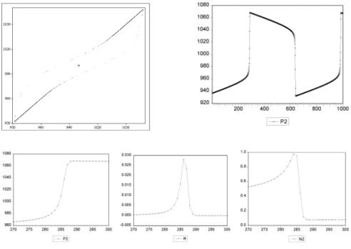
Fig. 1.
Top panel: Left figure: phase space projection of pricespt for deterministicskeleton without noise, wherept is plotted againstpt−1: coexisting limit cycle and
stable fundamental steady state p∗ = 1000 (marked as a square). Right figure:
corresponding time series along the limit cycle. Bottom panel: Time series of prices, returns, and fractions of trend followers. Parameter values:β= 2,r= 0.001,v= 1, g= 1.9, ¯y= 1,α= 1800,η= 0.99,aσ2= 1,δ
t≡0 andεt≡0.
The time series of the deterministic skeleton of prices, returns, and frac-tions of EMH believers along the cycle, as shown in the bottom pannel of fig-ure 1, yield important insight into the economic mechanism driving the price movements. Prices start far below the fundamental price p∗ = 1000. Since
the trend followers condition their trading rules upon the deviation from the fundamental price, the market will be dominated by EMH believers. Prices will slowly increase in the direction of the fundamental and the fraction of
19The memory parameter for all simulations in this paper isη= 0.99, so that for the
strategy selection decision past realized profits are slowly discounted. Simulations with other memory parameters yield similar results.
trend followers starts increasing. As the fraction of trend followers increases, the increase in prices is reinforced and trend followers earn a lot of money, which in turn causes the fraction of trend followers to increase even more, etc. At some critical phase from periods 283—288 prices rapidly move to a higher level. During this phase returns increase and volatility jumps to a high value, with a peak around period 286. As the price level moves to a high level of about 1070 far above the fundamental pricep∗ in period 288, the fraction of
trend followers drops to a low level of about 0.08, so that the market becomes dominated by EMH believers again. Prices decrease and move slowly in the direction of the fundamental price again20with small negative returns close to
zero and with low volatility. Thereafter, the fraction of trend followers slowly increases again, finally causing a rapid decrease in prices to a value of about 930, far below the fundamental, in period 640. Prices slowly move into the di-rection of the fundamental again to complete a full price (quasi)cycle of about 700 periods. The price cycle is thus characterized by a period of small changes and low volatility when EMH-believers dominate the market, and periods of rapid increase or decrease of prices with high volatility. The periods of rapid change and high volatility are triggered by technical trading; the conditioning of their charts upon the fundamental prevents the price to move too far away from the fundamental and leads to a new period of low volatility.
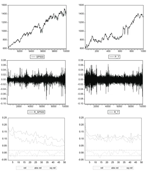
Adding dynamic noise to the system destroys the regularity of prices and returns along the cycle and leads to an irregular switching between phases of low volatility, with returns close to zero, and phases of high volatility, initiated by technical trading. Figure 2 compares time series observations of the same example buffeted with dynamic noise with daily S&P 500 data.21
Prices in our evolutionary model are highly persistent and close to having a unit root.22 In fact, simulated price series including only a sample size of
20In the case where all agents are EMH believers, the market equilibrium equation
without noise (13) reduces topt= (pt−1+rp∗)/(1+r), which is a linear difference
equation with fixed pointp∗and stable eigenvalue 1/(1+r), so that prices always
move slowly into the direction of the fundamental. Notice also that when all agents are EMH believers, the market equilibrium equation with noise (14) becomes
pt = (pt−1+rp∗+εt)/(1 +r), which is a stationary AR(1) process with mean
p∗ and root 1/(1 +r) close to 1, forrsmall. Hence, in the case when all traders
believe in a random walk, the implied actual law of motion is very close to a random walk and EMH-believers only make small forecasting errors which may be hard to detect in the presence of noise.
21The noise level was chosen high enough to destroy the regularity in the price
series such that autocorrelations in returns become insignificant for lags higher than one. But the noise should also not be too high in order not to destroy the structure imposed by the deterministic part of the model.
22Forv= 1 andr= 0 the characteristic polynomial of the Jacobian at the steady
state has an eigenvalue equal to 1. Note that the Jacobian of a linear difference equationyt=α0+PLk=1αkyt−khas an eigenvalue 1 if and only if the time series
600 800 1000 1200 1400 9200 9400 9600 9800 10000 SP500 600 800 1000 1200 1400 200 400 600 800 1000 P_T -0.10 -0.08 -0.06 -0.04 -0.02 0.00 0.02 0.04 0.06 0.08 2000 4000 6000 8000 10000 R_SP500 -0.10 -0.08 -0.06 -0.04 -0.02 0.00 0.02 0.04 0.06 0.08 2000 4000 6000 8000 10000 R_T
Fig. 2.
Daily S&P 500 data (left panel; prices: 07/11/1996—05/10/2000, returns: 08/17/1961—05/10/2000) compared with data generated by our model (right panel), with dynamic noiseεt∼ N(0,102) and other parameters as in figure 1: price series(top panel) return series (middle panel), and autocorrelation functions of returns, absolute returns, and squared returns (bottom panel).
1000 observations look ‘similar’ to real price series and the null hypothesis of a unit root is not rejected, though the series is generated by a stationary
model.23 24 The model price series exhibits sudden large movements, which
are triggered by random shocks and amplified by technical trading. (Notice the big price changes between periods 650 and 750 in the right top panel when prices are close to the fundamental p∗ = 1000, similar to the big changes in
the deterministic model, cf. figure 1.) When prices move too far away from the fundamental value 1000, technical traders condition their rule upon the fundamental and switch to the EMH-belief. With many EMH believers in the market, prices have a (weak) tendency to return to the fundamental value. As prices get closer to the fundamental, trend following behavior may become dominating again and trigger another fast price movement. However, in con-trast to the deterministic version of the model these big price movements do not occur regularly.
The middle panel of figure 2 compares return series of the S&P 500 over 40 years (where the October 1987 crash and the two days thereafter have been excluded25) with return series including 10000 observations generated by our
model. The simulated return series is qualitatively similar to the S&P 500 daily return series and exhibits clustered volatility.
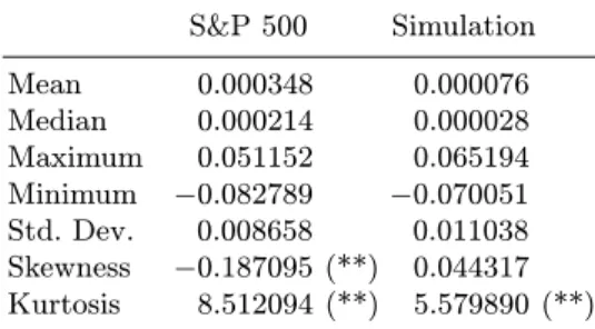
Table 1 shows some descriptive statistics for both return series. The means and medians of both return series are close to 0 and the range and standard de-viations are comparable in size. The S&P 500 returns have negative skewness, which is not the case in our example.26 This should not come as a surprise,
because our simple stylized model is in fact symmetric around the fundamen-tal steady state equilibrium, since both type of traders behave symmetrically with respect to high or low prices and with respect to positive or negative changes in prices. Finally, both return series show excess kurtosis, though the kurtosis coefficient of our example is smaller than the coefficients for the S&P 500 returns. This may be due to the fact that in our simple evolutionary system chartists’ price expectations are always conditioned upon the same distance function of price deviations from the fundamental price, i.e. upon
23For the price series presented in figure 2 test statistics for the simulated series are:
Augmented Dickey-Fuller:−0.8237 (S&P 500:−1.1858), Phillips-Perron:−0.8403
(S&P 500:−1.2238). The MacKinnon critical values for rejection of the hypothesis
of a unit root are: 1%: −3.4396, 5%:−2.8648, 10%:−2.5685.
24Notice that for price series with only 1000 observations the assumption of a
sta-tionary fundamental value seems quite reasonable. Whereas, if we would like to compare longer price series with real data we have to replace our IID dividend process by a non-stationary dividend process, e.g. by a geometric random walk. We intend to study such non-stationary evolutionary systems in future work.
25The returns for these days were about −0.20, +0.05, and +0.09. In particular,
the crash affects the autocorrelations of squared S&P 500 returns, which drop to small values of 0.03 or less for all lagsk ≥10 when the crash is included.
26Skewness statistics are not significant nor of the same sign for all markets.
Nev-ertheless, some authors examine the skewness in addition to excess kurtosis. [26] argue that skewness may be important in investment decisions because of induced asymmetries in realized returns.
the weighted distance (pt−1− p ) /αas described by (18). Nevertheless, our simple stylized evolutionary model clearly exhibits excess kurtosis.
Table 1.
Descriptive statistics for returns shown in figure 2. (**) null hypothesis of normality rejected at the 1% level.S&P 500 Simulation Mean 0.000348 0.000076 Median 0.000214 0.000028 Maximum 0.051152 0.065194 Minimum −0.082789 −0.070051 Std. Dev. 0.008658 0.011038 Skewness −0.187095 (**) 0.044317 Kurtosis 8.512094 (**) 5.579890 (**)
We next turn to the time series patterns of returns fluctuations and the phenomenon of volatility clustering. In real financial data autocorrelation functions (ACF) of returns are roughly zero at all lags. For high frequen-cies they are slightly negative for individual securities and slightly positive for stock indices. Autocorrelations functions of volatility measures such as ab-solute or squared returns are positive for all lags with slow decay for stock indices and a faster decay for individual stocks. This is the well-known stylized fact known as volatility clustering.
Figure 2 (bottom panel) shows autocorrelation plots of the first 50 lags of the return series and the series of absolute and squared returns. Both return series have significant, but small autocorrelations at the first lag (ρ1= 0.092
for the S&P 500 and ρ1 = 0.099 for our example). For the S&P 500 the
autocorrelation coefficient at the second lag is insignificant and at the third lag slightly negative significant (ρ2 = 0.005, ρ3 = −0.025), whereas in our
simulation the autocorrelation coefficient is small but significant at the second lag (ρ2= 0.070) and insignificant for the third lag (ρ3= 0.007). For all higher
order lags autocorrelations coefficients are close to zero and almost always insignificant. Our noisy conditional evolutionary model thus has almost no linear dependence in the return series.27
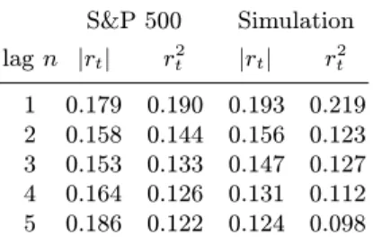
The bottom panel in figure 2 also shows that for the absolute and squared returns the autocorrelations coefficients of the first 50 lags are strongly sig-nificant and positive. Although our model is only six dimensional it is able to generate apparent long memory effects. Table 2 reports the numerical values
27[10] calibrate their evolutionary asset pricing model to ten years of monthly IBM
prices and returns. They present (noisy) chaotic time series with autocorrelations of prices and returns similar to the autocorrelation structure in IBM prices and returns. In particular, the noisy chaotic return series have (almost) no significant autocorrelations. However, these series do not exhibit volatility clustering, since there are no significant autocorrelations in squared returns.
of the autocorrelation coefficients at the first 5 lags, which are comparable in size for both series.
Table 2.
Autocorrelations of the absolute and squared returns shown in figure 2. S&P 500 Simulation lagn |rt| rt2 |rt| r2t 1 0.179 0.190 0.193 0.219 2 0.158 0.144 0.156 0.123 3 0.153 0.133 0.147 0.127 4 0.164 0.126 0.131 0.112 5 0.186 0.122 0.124 0.098Finally, we estimate a simple GARCH(1,1) model on the return series.28
As is well known, for many financial return series the sum of the ARCH(1) coefficient γ1 and the GARCH(1) coefficient γ2 is smaller than but close to
unity, representing the fact that the squared error term in the return equation follows a stationary, but highly persistent process. The estimated parameters are given in table 3.
Table 3.
GARCH(1,1) estimations for the returns shown in figure 2.γ1 γ2 γ1+γ2
S&P 500 0.069 0.929 0.998 Simulation 0.034 0.963 0.997
Our conditional evolutionary model thus exhibits long memory with long range autocorrelations and captures the phenomenon of volatility clustering. Let us finally briefly discuss the generality of the presented example. In order to get strong volatility clustering, the parameterv= 1 (orv very close to 1) is important, but the results are fairly robust with respect to the choices of the other parameter values.29 We find volatility clustering also for
para-meters where the fundamental value is a globally stable steady state. For parameter values close to the region where a stable steady state and a stable limit cycle coexist, price paths only converge slowly towards the fundamental value and look similar to price paths converging to a limit cycle. Especially,
28The estimations are done with EViews.
29As mentioned above, for v = 1 the system is close to having a unit root and
prices are highly persistent (cf. footnotes 22 and 23). [20] presents an example of strong volatility clustering for v= 0.9 for shorter time series. However, the null
when the system is buffeted with dynamic noise it is difficult to decide if parameters are chosen in or out of the global stability region.
In general, when 0 ≤ v < 1 volatility clustering becomes weaker, and sometimes also significant autocorrelations in returns may arise. The fact that v = 1 or v very close to 1 (so that type 1 are EMH-believers or fundamen-talists adapting only slowly into the direction of the fundamental), yields the strongest volatility clustering results may be understood as follows. When EMH-believers dominate the market asset prices are highly persistent and mean reversion is weak, since the evolutionary system is close to having a unit root (see footnote 20). Apparently, the interaction between unit root behav-ior far from the fundamental steady state with relatively small price changes driven only by exogenous news, and larger price changes due to amplification by trend following rules in some neighborhood around the fundamental price yields the strongest form of volatility clustering. We emphasize that all these results have been obtained for an IID dividend process and a corresponding constant fundamental price p∗. Including a non-stationary dividend process
and accordingly a non-stationary time varying fundamental process p∗ t may
lead to stronger volatility clustering also in the case 0≤ v <1. We leave this conjecture for future work.
5 Concluding Remarks
We have presented a nonlinear structural model for volatility clustering. Fluc-tuations in asset prices and returns are caused by a combination of ran-dom news about economic fundamentals and evolutionary forces. Two typical trader types have been distinguished. Traders of the first type are fundamen-talists (‘smart money’ traders), believing that the price of an asset returns to its fundamental value given by the discounted sum of future dividends or ‘EMH-believers,’ believing that prices follow a random walk. Traders of the second type are chartists or technical analysts, believing that asset prices are not solely determined by fundamentals, but that they may be predicted in the short run by simple technical trading rules based upon patterns in past prices, such as trends or cycles. The fraction of each of the two types is de-termined by an evolutionary fitness measure, given by accumulated profits, conditioned upon how far prices deviate from their fundamental value. This leads to a highly nonlinear, conditionally evolutionary learning model buffeted with noise.
The time series properties of our model are similar to important stylized facts observed in many real financial series. In particular, the autocorrelation structure of the returns and absolute and squared return series of our noisy nonlinear evolutionary system are similar to those observed in daily S&P 500 data, with little or no linear dependence in returns and high persistence and long memory in absolute and squared returns. Although the model is simple, it captures the first two moments of the distribution of real asset returns. Our
model thus might serve as a good starting point for a structural explanation — by a tractable model — of further stylized facts in finance, such as cross correlation between volatility and volume.
The generic mathematical mechanism generating volatility clustering is the coexistence of a stable fundamental steady state and a stable (quasi)perio-dic cycle. But there is also a strikingly simple economic intuition of why the phenomenon of volatility clustering should in fact be expected in our con-ditionally evolutionary system. When EMH-believers dominate the market prices are highly persistent, changes in asset prices are small and only driven by news, returns are close to zero and volatility is low. As prices move towards the fundamental, the influence of trend followers gradually increases, which reinforces the price trend. When trend followers start dominating the market, a rapid change in asset prices occurs with large (positive or negative) returns and high volatility. The price trend cannot persist forever, since prices cannot move away too far from the fundamental because technical traders condition their charts upon the fundamental. In the noisy conditionally evolutionary system both, the low and the high volatility phases, are persistent and the interaction between the two phases is highly irregular. The nonlinear interac-tion between heterogeneous trading rules in a noisy environment thus causes unpredictable asset returns and at the same time volatility clustering and the associated predictability in absolute and squared returns.
Our model is also able to explain empirical facts like ‘fat tails,’ i.e. it gen-erates excess kurtosis in the returns. This is due to the fact that the model implies a decomposition of returns into two terms, one martingale difference sequence part according to the conventional EMH theory, and an extra specu-lativeterm added by the evolutionary theory. The heterogeneity in the model thus creates excess volatility.
However, because of the simplicity of the model there are also some short-comings compared to real financial data, which we would like to discuss briefly. Our model does not generate return series which exhibit strong skewness. This is due to the fact that our agents use trading rules which are exactly sym-metric with respect to the constant fundamental value of the risky asset. As a consequence, the evolutionary model is also symmetric with respect to the fundamental price. Another shortcoming is that our model is stationary and therefore it is not able to generate long growing price series. By replacing our IID dividend process by a non-stationary dividend process, e.g. by a geomet-ric random walk, pgeomet-rices will also rapidly increase, similar to real series. We intend to study such non-stationary models within the presented framework in future work.30
Other important topics for future work are concerned with the welfare implications and the wealth distribution of our heterogeneous agents economy. What can be said about the total wealth in a multi-agent financial market where prices may (temporary) deviate from their fundamental compared to
the RE benchmark? How will wealth be distributed among traders? What would be an optimal investment strategy, a fundamentalists strategy, a trend following strategy or a switching strategy, in such a heterogeneous world? Notice that these are nontrivial questions, because although the number of trading types or strategies is only two in our setup, an underlying assumption of the discrete choice model for strategy selection is that the number of traders in the population is large, in fact infinite. To investigate wealth dynamics one thus has to keep track of the wealth distribution over an infinite population of traders. One could of course consider hypothetical wealth generated by a trader always sticking to the same type or strategy, but in our evolutionary world the majority of traders switch strategy in each time period based upon accumulated realized profits in the recent past. Addressing these important issues is beyond the scope of the present paper, but we plan to study welfare implications and wealth dynamics in future work.
In our model excess volatility and volatility clustering are created or rein-forced by the trading process itself, which seems to be in line with common financial practice. If the evolutionary interaction of boundedly rational, spec-ulative trading strategies amplifies volatility, this has important consequences for risk management and regulatory policy issues in real financial markets. Our model predicts that ‘good’ or ‘bad’ news about economic fundamentals may be amplified by evolutionary forces. Small fundamental causes may thus occasionally have big consequences and trigger large changes in asset prices. In the time of globalization of international financial markets, small shocks in fundamentals in one part of the world may thus cause large changes of asset prices in another part of the world. Our simple structural model shows that a stylized version of this theory already fits real financial data surprisingly well. Our results thus call for more financial research in this area to build more re-alistic models to asses investors’ risk to speculative trading and evolutionary amplification of changes in underlying fundamentals.
References
1. Anderson, S., de Palma, A. and Thisse, J. (1993). Discrete Choice Theory of Product Differentiation. MIT Press, Cambridge.
2. Arifovic, J. and Gencay, R. (2000). Statistical properties of genetic learning in a model of exchange rate. Journal of Economic Dynamics and Control
24
, 981—1005.3. Arthur, W.B., Holland, J.H., LeBaron, B., Palmer, R. and Taylor, P. (1997). Asset pricing under endogenous expectations in an artificial stock market, in: Arthur, W.B., Durlauf, S.N., and Lane, D.A. (Eds.),The Economy as an Evolv-ing Complex System II. Redwood City, Addison-Wesley, pp. 15—44.
4. Baillie, R.T., Bollerslev, T. and Mikkelsen, H.O. (1996). Fractionally integrated generalized autoregressive conditional heteroskedasticity.Journal of Economet-rics
74
, 3—30.5. Bollerslev, T. (1986). Generalized autoregressive conditional heteroscedasticity. Journal of Econometrics
31
, 307—327.6. Breidt, F.J., Crato, N. and de Lima, P. (1998). The detection and estimation of long memory in stochastic volatility.Journal of Econometrics
83
, 325—348 . 7. Brock, W.A. (1993). Pathways to Randomness in the Economy: EmergentNon-linearity and chaos in economics and finance.Estudios Econ´omicos
8
, 3—55. 8. Brock, W.A. (1997). Asset price behavior in complex environments, in: Arthur,W.B., Durlauf, S.N., and Lane, D.A. (Eds.),The Economy as an Evolving Com-plex System II. Addison-Wesley, Reading, MA, pp. 385—423.
9. Brock, W.A. and Hommes, C.H. (1997). A rational route to randomness. Econo-metrica
65
, 1059—1095.10. Brock, W.A. and Hommes, C.H. (1997). Models of complexity in economics and finance, in: Hey, C., Schumacher, J.M., Hanzon, B., and Praagman, C. (Eds.), System Dynamics in Economic and Financial Models. John Wiley & Sons, Chichester, pp. 3—41.
11. Brock, W.A. and Hommes, C.H. (1998). Heterogeneous beliefs and routes to chaos in a simple asset pricing model.Journal of Economic Dynamics and Con-trol
22
, 1235—74.12. Chiarella, C. (1992). The dynamics of speculative behaviour.Annals of Opera-tions Research
37
, 101—123.13. DeGrauwe, P., DeWachter, H. and Embrechts, M. (1993).Exchange rate theory. Chaotic models of foreign exchange markets. Blackwell, Oxford.
14. DeGrauwe, P. and Grimaldi, M. (2004). Exchange rate puzzles: a tale of switch-ing attractors,Working paper, University of Leuven.
15. Engle, R.F. (1982). Autoregressive conditional heteroscedasticity with estimates of the variance of United Kingdom inflation.Econometrica
50
, 987—1007. 16. Farmer, J.D. and Joshi, S. (2002). The price dynamics of common tradingstrate-gies.Journal of Economic Behavior & Organization
49
, 149—171.17. de Fontnouvelle, P. (2000). Information dynamics in financial markets. Macro-economic Dynamics
4
, 139—169.18. Frankel, J.A. and Froot, K.A. (1986). Understanding the US Dollar in the Eight-ies: the Expectations of Chartists and Fundamentalists.Economic Record, Spe-cial Issue 1986, 24—38.
19. Gaunersdorfer, A. (2000). Endogenous fluctuations in a simple asset pricing model with heterogeneous beliefs. Journal of Economic Dynamics and Control
20. Gaunersdorfer, A. (2001). Adaptive Beliefs and the Volatility of Asset Prices. Central European Journal of Operations Research
9
, 5—30.21. Gaunersdorfer A. and Hommes C.H. (2000). A Nonlinear Structural Model for Volatility Clustering — Working Paper Version. SFB Working Paper No. 63, University of Vienna and Vienna University of Economics and Business Admin-istration, andCeNDEF Working PaperWP 00-02, University of Amsterdam. 22. Gaunersdorfer, A., Hommes, C.H. and Wagener, F.O.J. (2003). Bifurcation
routes to volatility clustering under evolutionary learning. CeNDEF Working
Paper03-03, University of Amsterdam.
23. Goetzmann, W. and Massa, M. (2000). Daily Momentum and Contrarian Be-havior of Index Fund Investors.Journal of Financial and Quantitative Analysis, forthcoming.
24. Granger, C.W.J. and Ding, Z. (1996). Varieties of long memory models.Journal of Econometrics
73
, 61—77.25. Grossman, S. and Stiglitz, J. (1980). On the impossibility of informationally efficient markets. American Economic Review
70
, 393—408.26. Harvey C.R. and Siddique A. (2000). Conditional Skewness in Asset Pricing Tests.Journal of Finance
55
, 1263—1295.27. Hirshleifer, D. (2001). Investor Psychology and Asset Pricing. Journal of Fi-nance
56
, 1533—1597.28. Hommes, C.H. (2001). Financial markets as nonlinear adaptive evolutionary systems. Quantitative Finance
1
, 149—167.29. Hommes, C.H. (2002). Modeling the stylized facts in finance through simple nonlinear adaptive systems.Proc. Nat. Ac. Sc.
99
, 7221—7228.30. Kirman, A. (1991). Epidemics of opinion and speculative bubbles in financial markets, in: Taylor, M. (Ed.),Money and Financial Markets. Macmillan, Lon-don, pp. 354—368.
31. Kirman, A. (1998). On the nature of gurus.mimeo, GREQAM, Marseille. 32. Kirman, A. and Teyssi`ere, G. (2002). Microeconomic models for long memory in
the volatility of financial time series. Studies in Nonlinear Dynamics & Econo-metrics
5
, 281—302.33. Kuznetsov, Y.A. (1998). Elements of Applied Bifurcation Theory (2nd ed.). Springer Verlag, New York.
34. Kyle, A.S. (1985). Continuous Auctions and Insider Trading.Econometrica
53
, 1315—1335.35. LeBaron, B., Arthur, W.B. and Palmer, R. (1999). Time series properties of an artificial stock market.Journal of Economic Dynamics and Control
23
, 1487— 1516.36. Lo, A.W. and MacKinlay, A.C. (1990). When Are Contrarian Profits Due to Stock Market Overreaction?The Review of Financial Studies
3
, 175—205. 37. Lux, T. (1995). Herd Behavior, Bubbles and Crashes. The Economic Journal105
, 881—896.38. Lux, T. and Marchesi, M. (1999). Scaling and criticality in a stochastic multi-agent model of a financial market.Nature
397
, 498—500.39. Lux, T. and Marchesi, M. (2000). Volatility Clustering in Financial Markets: A Microsimulation of Interacting Agents.International Journal of Theoretical and Applied Finance
3
, 675—702 .40. Mandelbrot, B. (1963). The variation of certain speculative prices.Journal of Business
36
, 394—419.41. Mandelbrot, B. (1997).Fractals and Scaling in Finance: Discontinuity, Concen-tration, Risk. Springer Verlag, New York.
42. Mandelbrot, B. (1999). A multi-fractal walk down Wall Street.Scientific Amer-ican,
280 (2)
, 50—53.43. Manski, C. and McFadden, D. (1981).Structural analysis of discrete data with econometric applications. MIT Press, Cambridge.
44. Manzan, S. (2003). Essays in Nonlinear Economic Dynamics.Thesis, University of Amsterdam.
45. Pagan, A. (1996). The Econometrics of Financial Markets,Journal of Empirical Finance
3
, 15—102.46. Palis, J. and Takens, F. (1993).Hyperbolicity and Sensitive Chaotic Dynamics at Homoclinic Bifurcations. Cambridge University Press, New York.
47. Routledge B.R. (1999). Adaptive Learning in Financial Markets.The Review of Financial Studies
12
, 1165—1202.48. Shefrin, H. (2000).Beyond greed and fear. Understanding behavioral finance and the psychology of investing. Harvard Business School Press, Boston.
49. Shleifer, A. (2000). Inefficient markets. An introduction to behavioral finance. Clarendon Lectures in Economics, Oxford University Press.
50. Timmermann, A. (1993). How learning in financial markets generates excess volatility and predictability in stock prices. Quarterly Journal of Economics
108
, 1135—1145.51. Timmermann, A. (1996). Excess volatility and predictability of stock prices in autoregressive dividend models with learning. Review of Economic Studies
63
, 523—557.52. Woodford, M. (2000). An interview with William A. Brock. Macroeconomic Dynamics
4
, 108—138.53. Youssefmir, M. and Huberman, B.A. (1997). Clustered volatility in multiagent dynamics.Journal of Economic Behavior & Organization