A FULL COVERAGE FILM COOLING STUDY: THE
EFFECT OF AN ALTERNATING COMPOUND
ANGLE
by
JUSTIN HODGES
B.S. Mechanical Engineering, University of Central Florida, 2012
A thesis submitted in partial fulfillment of the requirements
for the degree of Master of Science
in the Department of Mechanical, Materials and Aerospace Engineering
in the College of Engineering and Computer Science
at the University of Central Florida
Orlando, Florida
Spring Term
2015
ABSTRACT
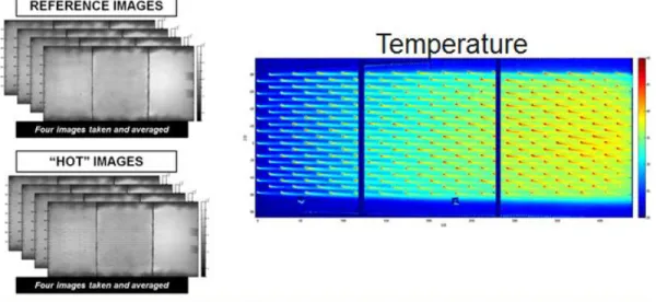
This thesis is an experimental and numerical full-coverage film cooling study. The objective of this work is the quantification of local heat transfer augmentation and adiabatic film cooling effectiveness for two full-coverage film cooling geometries. Experimental data was acquired with a scientific grade CCD camera, where images are taken over the heat transfer surface, which is painted with a temperature sensitive paint. The CFD component of this study served to evaluate how well the v2-f turbulence model predicted film cooling effectiveness throughout the array, as compared with experimental data.
The two staggered arrays tested are different from one another through a compound angle shift after 12 rows of holes. The compound angle shifts from β=-45° to β=+45° at row 13. Each geometry had 22 rows of cylindrical film cooling holes with identical axial and lateral spacing (X/D=P/D=23).
Levels of laterally averaged film cooling effectiveness for the superior geometry approach 0.20, where the compound angle shift causes a decrease in film cooling effectiveness. Levels of heat transfer augmentation maintain values of nearly h/h0=1.2. There is no effect of compound angle shift on heat transfer augmentation observed. The CFD results are used to investigate the detrimental effect of the compound angle shift, while the SST k-ω turbulence model shows to provide the best agreement with experimental results.
For my Dad. You dedicated years of your life selflessly to show me what it means to be a man.
From you, I have been afforded an amazing gift; I have become a man I am very proud to be.
Any result I may produce is poorly represented without attribution to your influence in my
life.
For my Mom. You have shown me the power and benefit of steadfast commitment to an idea,
a set of ethics, and tireless patience. You have instilled in me a non-temporal conviction to
treat others with respect, and have raised me to value a relationship with Christ.
To Jordan, Glen, Tegan, and Amy. Every friendship pales in comparison, the last 7 years
describe what most would define as ‘what it means to feel alive’.
ACKNOWLEDGMENTS
My sincere gratitude extends to my adviser, Dr. Jayanta Kapat. Years ago I was
required to meet with a faculty member in the Engineering department, as per the
curriculum, and ‘happened’ to meet with you. From the moment I sat in your office and
listened to you talk about your lab and describe your students work, I knew I had to be a
part of it. Since that hour, working in your group has been one of the best experiences I
have had. I have thoroughly enjoyed the challenging moments, the rewarding moments,
the friendships that have ensued, the doors that have opened for me professionally, and
most certainly the struggle. Thank you for all that you have done, I look to the future with
great excitement and anticipation!
I am happy to have the opportunity to thank Dr. Michael Crawford for his
incredible knowledge and leadership throughout the years. It has been an absolute
blessing to work with such a name. I attribute much of my professional growth to the
projects we collaborated on. Also, I would like to especially thank Ken Landis, Glenn
Brown, Dr. Rodriguez, and Dr. DeSilva from Siemens for the knowledge I have received, by
virtue of our work together!
I would also like to greatly thank Dr. Ali Gordon and Dr. Subith Vasu for being on
my thesis committee. I sincerely appreciate your guidance through this process.
I must also strongly thank Greg Natsui for his outstanding leadership as my direct
mentor over the past few years. We have spent countless hours working together, and I
am very lucky to have had such great development professionally, intellectually, and as a
person because of you. Some of the best moments of understanding were with you, a
textbook, some scratch paper and a felt pen, and MATLAB.
Thank you Mark Ricklick for the most embarrassing, humiliating, and character
building moment in my professional career, as you grilled me for about 15 minutes
straight in front of everybody at the lab, just after I started working there. That moment
was quite a turning point for my professional attitude, as I have never been so strict on
myself for understanding fundamentals and holding myself to a higher standard. I am
genuinely grateful for that moment and our friendship. Also, thank you for being so awful
at fishing that I get the chance to teach you and hold countless discussions with you on
how to not be so awful at fishing.
To the world’s best lab mates - Matt Golsen, Roberto, Anthony Bravato, Lucky,
Patrick, Jahed (you can do anything), Brandon, Malay (GW2 champion), Constantine, Josh
Schmitt, Josh Bernstein, Sri, Barkin (worst soccer player of all time), Marcel, Dr. Wang,
Lumaya, Marc Medina (forever weak), Lauren, Chris V, Rachel, Perry, Christian Garrett
(best work study student of all time), Joe, Craig, Daniel Gonzalez, Ahmed, Sergio, Bryan
Bernier, Luke, John Harrington, and many others. You all made it very easy to spend so
much time in a LABORatory!
I am also very thankful to work with Tyler Voet and Stephen Stafstrom. Two great
jedi padawan learners who make work less stressful and even more fulfilling.
I have made a lot of great friendships through work in the past few years, but I
would like to particularly show appreciation for the friendship and collaborative work
Zach Little and I have experienced. I really appreciate all the support from you, you are a
great friend and colleague!
A big thanks belongs to Cassandra Carpenter for also being an amazing mentor.
Your kindness, knowledge, guidance, and enthusiasm did/does not go unappreciated. You
are an ideal breed for working with and managing people, and also a great friend. I hold
great value in my newly found love for CFD, and I cannot go without thanking you for
everything you have taught me while starting out.
TABLE OF CONTENTS
LIST OF FIGURES
xiii
LIST OF TABLES
xviii
LIST OF EQUATIONS
xix
NOMENCLATURE
xxii
CHAPTER 1: INTRODUCTION AND LITERATURE REVIEW
1
1.1 The Motivation to Study Gas Turbines 1
1.2 Basis of Gas Turbine Operation 1
1.3 Gas Turbine Cooling and Heat Transfer 2
1.3.1 Convective Cooling 4
1.3.2 Impingement Cooling 4
1.3.3 Film Cooling 5
1.4 Film Cooling Basics and Literature Review 6
1.4.1 Geometric Parameters Influencing Film Cooling 6
1.4.2 Independent Parameters Used in Film Cooling 12
1.4.3 Full Coverage Film Cooling 15
1.4.3.2 Full-Coverage Film Cooling Part I: Comparison of Heat Transfer Data for Three Injection
Angles [18] 17
1.4.3.3 Full-Coverage Film Cooling Part I: Comparison of Heat Transfer Data for Three Injection
Angles [19] 18
1.4.3.4 An Investigation of the Heat Transfer for Full Coverage Film Cooling [20] 18 1.4.3.5 Film Cooling Effectiveness for Injection from Multirow Holes [21] 18 1.4.3.6 Turbulence intensity effects on film cooling and heat transfer from compound angle holes
with particular application to gas turbine blades [22] 19
1.4.3.7 Film cooling from two rows of holes with opposite orientation angles: injectant behavior
and adiabatic film cooling effectiveness [23] 19
1.5 Scope and Objective of Current Study 20
CHAPTER 2: EXPERIMENTAL SETUP AND TESTING PREPARATION
21
2.1 Geometries Tested 21
2.1.1 Independent Testing Parameters Which Influence Film Cooling 21
2.1.2 Test Matrix 25
2.1.3 Machining Process 26
2.1.4 Geometric Uncertainty 29
2.2 Wind Tunnel 30
2.2.1 Blowers 31
2.2.2 Wind Tunnel Flow Measurements 31
2.3.1 Testing Methodology – Adiabatic Film Cooling Effectiveness 36
2.3.2 Testing Methodology – Heat Transfer Augmentation 39
2.4 Uncertainty Quantification 50
CHAPTER 3: ADIABATIC FILM COOLING EFFECTIVENESS RESULTS
54
3.1 Benchmark 54
3.2 Local Physics 54
3.3 Laterally Averaged Film Cooling Effectiveness 56
3.3.1 FC.V 58
3.3.2 FC.VI 61
3.3.3 Direct Comparisons between Geometries 62
CHAPTER 4: HEAT TRANSFER AUGMENTATION RESULTS
64
4.1 Benchmark 64
4.2 Local Heat Transfer Augmentation 67
4.3 Span Average Heat Transfer Augmentation 69
4.3.1 FC.VI 69
CHAPTER 5: COMPUTATIONAL EFFORTS
71
5.1.1 Geometry 71
5.2 Mesh 74
5.3 Boundary Conditions 82
5.4 Generic Physics Models 85
5.4.1 Gradients 86
5.4.2 Hybrid LSQ Method 87
5.4.3 Ventkatakrishnan Limiter Method 87
5.4.4 Segregated Flow 88
5.4.5 Segregated Fluid Temperature 89
5.4.6 Miscellaneous Models 89
5.4.7 Initial Conditions 89
5.5 Turbulence Models 90
5.5.1 V2-f Variant of the Traditional K-ε Model 94
5.5.2 SST Variant of the K-ω Model 98
5.6 Resources 101
5.7 Results and Discussion (FC.VI, M=1.0) 101
CHAPTER 6: CONCLUDING REMARKS
111
6.1 Film Cooling Effectiveness 111
LIST OF FIGURES
Figure 1: Various popular cooling schemes in gas turbines [2] ... 3
Figure 2: Description of inclination and compound angle with sign convention ... 11
Figure 3: Description of lateral pitch (P) and streamwise pitch (X) ... 12
Figure 4: The general effect of momentum flux ratio on jet lift off ... 14
Figure 5: Literature geometric parameters compared with current study [34 -50]... 16
Figure 6: Coordinate system and nomenclature for angles describing film hole geometry ... 22
Figure 7: Geometric parameters describing an array of film cooling holes ... 23
Figure 8: Geometric parameters describing an array of film cooling holes ... 23
Figure 9: The general effect of momentum flux ratio, describing lift off... 25
Figure 10: CAD drawings for a HTC test geometry with ... 26
Figure 11: Plates were machined using a CNC ... 27
Figure 12: The spindle was rotated to achieve the desired hole inclination angle ... 27
Figure 13: A fixture was made to hold the plates at the appropriate orientation angles (for machining the compounding angle) ... 28
Figure 14: Test surface composed of three sections (plates) ... 29
Figure 15: Geometric uncertainty table ... 29
Figure 16: Experimental setup of heat transfer surface, comprised of three separate plates ... 30
Figure 17: Wind tunnel (crossflow) and plenum (secondary flow) for large film cooling array studies ... 31
Figure 18: Static pressure variation in the stream-wise direction of the duct without the pressure insert in the wind tunnel ... 32
Figure 19: CTA velocity measurements of the boundary layer for the maximum tunnel free stream velocity ... 34
Figure 20: CTA velocity measurements of the boundary layer for a low tunnel free stream ... 35
Figure 21: Inner scaling of boundary layer for the tunnels maximum free stream velocity ... 35
Figure 22: Inner scaling of boundary layer for a lower tunnel free stream velocity ... 36
Figure 23: Adiabatic film cooling effectiveness experimental setup ... 37
Figure 24: Process of processing temperature from raw data using TSP ... 38
Figure 25: Typical calibration curve for TSP (in-house) ... 39
Figure 26: Heat transfer augmentation experimental setup ... 40
Figure 27: Stainless steel type 321 temperature vs. electrical resistivity ... 42
Figure 28: Control volume and energy balance of heater surface ... 43
Figure 29: Conduction heat loss test setup ... 44
Figure 30: Conduction heat loss test results ... 45
Figure 31: Radiation heat loss results ... 46
Figure 32: Cartoon image of circuit measurement devices ... 49
Figure 33: Heated and unheated surfaces and the effect on heat transfer ... 50
Figure 34: Contributions to uncertainty in heat transfer coefficient ... 51
Figure 35: Contributions to uncertainty in adiabatic film-cooling effectiveness ... 51
Figure 36: Contributions to uncertainty in blowing ratio ... 52
Figure 37: Comparison of in-house data vs. Mayle (1975) ... 54
Figure 38: Adiabatic film cooling effectiveness (local data) for FC.V at all blowing ratios ... 55
Figure 39: Adiabatic film cooling effectiveness (local data) for FC.VI at all blowing ratios ... 56
Figure 40: Sample data (from this work) with contours and the averaging window for laterally averaged effectiveness shown ... 58
Figure 42: Comparison of effectiveness data for different freestream velocities, for FC.V, M=0.5 ... 60
Figure 43: Comparison of effectiveness data for different freestream velocities, for FC.V, M=1.0 ... 60
Figure 44: Comparison of effectiveness data for different freestream velocities, for FC.V, M=2.0 ... 61
Figure 45: FC.VI Adiabatic Film Cooling Effectiveness ... 62
Figure 46: FC.V and FC.VI effectiveness compared for all blowing ratios ... 63
Figure 47: Flat plate h0 validation ... 64
Figure 48: Validation of the M=0.5 case with (identical geometry) Mayle [3] ... 65
Figure 49: Validation of the M=1.0 case with (identical geometry) Mayle [3] ... 65
Figure 50: Validation of the M=1.5 case with (identical geometry) Mayle [3] ... 66
Figure 51: h0 testing, comparing of experiment and correlation ... 67
Figure 52: Local HTC augmentation values for FC.VI at all blowing ratios ... 68
Figure 53: FC.VI heat transfer data for M=0.50 ... 69
Figure 54: FC.VI heat transfer data for M=1.0 ... 70
Figure 55: FC.VI heat transfer data for M=2.0 ... 70
Figure 56: Isometric view of the fluid domain ... 71
Figure 57: Top view of geometry ... 71
Figure 58: Side view of geometry ... 71
Figure 59: Region defined for fluid domain ... 73
Figure 60: Fluid domain showing mesh transition from fine near heat transfer surface to coarse in free-stream ... 75
Figure 61: Domain showing recursive pattern of fine and coarse mesh in streamwise direction ... 75
Figure 62: Image on left shows filler block located between rows of holes, and image on right shows block located directly above holes ... 76
Figure 64: Cell quality over wall normal plane to heat transfer surface (from 0 to 1) ... 78
Figure 65: Histogram of cell quality (quality ranging from 0 to 1, and number of cells ranging from 106 to 1.2*107) ... 79
Figure 66: Histogram of skewness angle (skewness angle from 0 to 90, number of cells from 2*106 to 22*106) ... 80
Figure 67: Histogram of volume change metric (volume change from 0.001 to 1, number of cells from 100 to 1*108)... 81
Figure 68: Wall y+ value distribution on the heat transfer surface ... 81
Figure 69: Side view of fluid domain indicating location of the select boundaries ... 82
Figure 70: Top view of domain with location of hole sections highlighted ... 83
Figure 71: Top view of domain showing location of internal interface for periodic boundary condition ... 85
Figure 72: General tree line of the simulation ... 86
Figure 73: Initial Conditions listed in STAR-CCM+ ... 90
Figure 74: Comparison of experimental data and V2f CFD predictions (FC.VI, M=1) ... 104
Figure 75: Comparison of experimental data and SST CFD predictions (FC.VI, M=1) ... 105
Figure 76: Comparison of experimental data and EBKE CFD predictions (FC.VI, M=1) ... 106
Figure 77: Comparison of 3 turbulence models performance with experimental data ... 107
Figure 78: FC.II M=1.0 residual per iteration for the first 7k iterations in the simulation ... 108
Figure 79: Average static temperature over the heat transfer surface as per iteration ... 110
Figure 80: Comparison of laterally averaged effectiveness for several test cases at all blowing ratios ... 112 Figure 81: Local film cooling effectiveness at the compound angle shift for FC.V at the high and low
LIST OF TABLES
Table 1: Inclination angles used in studies compiled in Bunker's [12] review ... 9
Table 2: Geometric test speciman matrix for current study ... 25
Table 3: Flow measurements for wind tunnel with constant temperature anemometry ... 33
Table 4: Experimental uncertainty for heat transfer coefficient and augmentation, and effectiveness ... 53
Table 5: Experimental uncertainty in intermediate parameters ... 53
Table 6: Sample quantities used for FC.VI, M=1 computation ... 73
Table 7: Mesh settings ... 77
Table 8: Tabulated quantities for boundary conditions ... 83
Table 9: Crossflow inlet quantities for boundary condition specification ... 84
Table 10: Crossflow exit quantities for boundary condition specification ... 84
Table 11: Coefficients used for the V2f turbulence model testing ... 98
LIST OF EQUATIONS
Equation 1: Density Ratio ... 13
Equation 2: Blowing Ratio ... 13
Equation 3: Momentum Flux Ratio... 14
Equation 4: Blowing Ratio ... 24
Equation 5: Density Ratio ... 25
Equation 6: Momentum Flux Ratio... 25
Equation 7: Input Heat Flux ... 43
Equation 8: Electrical Heater Resistance ... 44
Equation 9: Heat loss as a Function of Wall Temperature ... 45
Equation 10: Radiation Heat Loss of the Experimental Rig ... 47
Equation 11: Local, Uncorrected Heat Transfer Coefficient ... 47
Equation 12: Corrected Convective Heat Flux ... 47
Equation 13: Corrected Heat Transfer Coefficient (Effectiveness Utilized) ... 47
Equation 14: Nusselt Number Flat Plate Correlation ... 50
Equation 15: Nusselt Number Correlation Involving an Unheated Starting length ... 50
Equation 16: Uncorrected Heat Transfer Coefficient Without Blowing ... 50
Equation 17: Heat Transfer Coefficient Augmentation Factor ... 50
Equation 18: Experimental Uncertainty ... 52
Equation 19: Film Cooling Effectiveness ... 57
Equation 20: Laterally Averaged Film Cooling Effectiveness ... 57
Equation 21: Weighted Least Squares Formula for Gradient Reconstruction ... 87
Equation 23: Discretized Continuity ... 88
Equation 24: Total Energy ... 89
Equation 25: Continuity ... 91
Equation 26: Momentum ... 91
Equation 27: Energy ... 91
Equation 28: RANS ... 92
Equation 29: Energy with RANS Decomposition ... 92
Equation 30: Reynolds Stress (Fluctuations in Momentum due to Turbulence) ... 92
Equation 31: Turbulent Heat Flux from RANS Decomposition ... 92
Equation 32: Reynolds Stress Defined in Terms of Eddy Diffusivity ... 93
Equation 33: Turbulent Heat Flux from RANS Decomposition in Terms of Eddy Diffusivity ... 93
Equation 34: RANS with Eddy Diffusivity Incorporated ... 93
Equation 35: Energy Equation with RANS Decomposition and Eddy Diffusivity Incorporated ... 93
Equation 36: Eddy Viscosity ... 94
Equation 37: Turbulent Transport Equation No. 1 for V2f ... 95
Equation 38: Turbulent Transport Equation No. 2 for V2f ... 95
Equation 39: V2f Definition of Eddy Viscosity ... 96
Equation 40: Transport Equation No. 3 for V2f ... 96
Equation 41: Elliptic Relaxation for 'f' in V2f Model ... 96
Equation 42: Length Scale (V2f Specific) ... 97
Equation 43: Time Scale (V2f Specific) ... 97
Equation 44: Eddy Viscosity (Specific to the K- ω Model)... 98
Equation 46: Transport Equations for the K-ω Model ... 99
Equation 47: Transport Equation No. 1 for the SST K- ω Model... 100
Equation 48: Transport Equation No. 2 for the SST K- ω Model... 100
NOMENCLATURE
Symbols
Ac Cross-sectional area As Surface area D Hole diameter DR Density ratio; 𝐷𝑅 = 𝜌𝑐⁄𝜌∞=𝑇∞⁄ (𝑓𝑜𝑟 𝑡𝑤𝑜 𝑠𝑖𝑚𝑖𝑙𝑎𝑟 𝑖𝑑𝑒𝑎𝑙 𝑔𝑎𝑠𝑒𝑠)𝑇𝑐EBKE Elliptic Blending k-ε turbulence model
hu Uncorrected heat transfer coefficient
hf Corrected heat transfer coefficient (corrected for film temperature)
h0 Heat transfer coefficient without blowing
i Current
I Momentum flux ratio; 𝐼 = (𝜌𝑢2)𝑐⁄(𝜌𝑢2)∞=𝑀2⁄𝐷𝑅
k Thermal conductivity
kf Thermal conductivity of air
L Hole axis length
M Blowing ratio; 𝑀 = (𝜌𝑢)𝑐⁄(𝜌𝑢)∞
Nux Nusselt number; 𝑁𝑢𝑥 = ℎ0𝑥 𝑘⁄ 𝑓
Nx Number of streamwise rows
Nz Number of spanwise holes
P Lateral pitch between holes, measured exit breakout to adjacent exit breakout
Pr Prandtl number
q”f Heat flux in the presence of film cooling
q”conv Heat flux loss by convection
q”cond Heat flux loss by conduction
q”rad Heat flux loss by radiation
q”gen Heat flux generated by joule heating
R Resistance
Re Film cooling Reynolds number; 𝑅𝑒 = 𝑈∞𝐷 𝜈⁄
Rex Reynolds number based on x; 𝑅𝑒 = 𝑈∞𝑥 𝜈⁄
s Equivalent slot width; 𝑠 = 𝜋𝐷 4(𝑃 𝐷⁄ ⁄ )
SST Menter’s Shear Stress Transport turbulence model
t Thickness
T Temperature
Taw Adiabatic wall temperature
Tb Backside temperature driving conduction
Tc Coolant temperature
Tref Temperature of reference picture
Tw Wall temperature
T∞ Freestream temperature
TI Turbulence intensity; TI=u’2rms/U
u[ ] Total uncertainty of [ ]
u, v, w Corresponding stream, wall normal, and lateral velocities
U Velocity magnitude
U∞ Freestream velocity magnitude
x, y, z Stream, wall normal, lateral (spanwise)
X Streamwise pitch, measured exit breakout to projected exit breakout
y+ Inner scaled wall normal coordinate;𝑦+= (𝑦√𝜏0⁄ ) 𝜈𝜌 ⁄
Greek
α Inclination angle
β Compound angle
η Adiabatic film cooling effectiveness; 𝜂 = (𝑇∞− 𝑇𝑎𝑤) (𝑇⁄ ∞− 𝑇𝑐)
θ Non-dimensional temperature between coolant, freestream and heater
ξi Unheated starting length distance ‘i’ for calculation of h0
ρel Electrical resistivity
ρc Coolant density
ρ∞ Freestream density
σ Stephan Boltzmann constant
Acronyms
CATER Center for Advanced Turbines and Energy Research
CFD Computational fluid dynamics
CCD Charged coupled device
CTA Constant temperature anemometer (hot-wire)
FCFC Full coverage film cooling (followed by; I – FY2010, II – FY2011)
FPG Favorable pressure gradient
IR Infrared
RANS Reynolds Averaged Navier Stokes
RR Recovery region
TKE Turbulent kinetic energy
CHAPTER 1: INTRODUCTION AND LITERATURE REVIEW
1.1
The Motivation to Study Gas Turbines
Gas turbine technology is widely used throughout many applications, most notably in land based power generation, aviation, and marine applications. The design of gas turbines represents one of the most exciting and challenging problems of the current age, utilizing experts of many disciplines. Research in gas turbine systems is driven by their economic and environmental impact, these machines which produce over 90% of the world's power and propel near 100% of commercial aviation [1]. Even though completely renewable energy has been given significant attention in recent years, gas turbines fired from coal and natural gas will continue to produce the majority of the world's power into the foreseeable future. This suggests that a natural step towards efficiently utilizing our natural resources is improving gas turbine technology, both for land based power generation and aviation. Such
statements warrant the need for study and motivation to study.
1.2 Basis of Gas Turbine Operation
The basis of a gas turbine is to provide a thermodynamic system which results in a positive of transfer of work using air and fuel mixtures for combustion. This positive work transfer is used in combination with generators for generating electricity, then distributed to the where the needs exists within the electrical grid network (e.g. houses, buildings, etc.). The main components in a general, basic (open) gas turbine are a compressor, combustor, and turbine. Work input is required by the compressor, as ambient air enters the gas turbine system through the compressor. After carefully compressed, the air is introduced into combustion chambers with a foreign species (fuel) for combustion. Upon combustion, the air-fuel mixture has a significant increase in temperature and
volume per unit mass, where it then enters and expands throughout the turbine section. This expansion process through the turbine is the process by which the fluid does work on the turbine blades, thus creating a positive transfer of work. Resources (e.g. work input to compressor, fuel, etc.) are successfully leveraged when the work provided through the turbine section exceeds the work required to elsewhere in the gas turbine configuration.
This process describing gas turbine operation is known as the Brayton cycle. The ideal Brayton cycle consists of: 1. isentropic compression, 2. isobaric heat addition, 3. isentropic expansion, and 4. isobaric heat extraction.
An increase in thermodynamic efficiency of the engine is dominated by engine pressure ratio and increasing the firing temperature. It is the goal of gas turbine heat transfer research to enable this firing temperature to rise even higher than the already greater than melting temperature of the gas turbine components, such that higher efficiencies can be achieved. This is a multi-discipline effort however, where many groups of experts are working to safely increase turbine firing temperatures with different technologies; new material technologies which better protect turbine walls/blades (e.g. thermal barrier coatings), various internal cooling techniques throughout turbine blade passages (e.g. impingement cooling), and several external cooling techniques over the blades (e.g. film cooling), to name a few.
1.3
Gas Turbine Cooling and Heat Transfer
As described previously, there is a clear need to increase firing temperatures in gas turbines such that higher efficiencies can be achieved, and thus human resources can be spent slower at more sustainable rates. As a result, the effort to increase firing temperatures in gas turbines is relentless and ever-growing.
Earlier in the 20th century, gas turbine technology was such that operation could presume
without the dedicated, elegant cooling systems that exist today. At that time, the capabilities in high firing temperatures were lacking such that the alloys used in combustor and turbine sections could withstand thermal loads driven by the hot gas path. Given the multidisciplinary effort of increasing gas turbine efficiency, and thus increasing combustion and hot gas path temperatures, eventually more advanced and dedicated cooling systems (in cooperation with metallurgical advances) were required to maintain the integrity of the components within gas turbines.
Several popular cooling schemes are used for protecting critical regions subject to high temperatures; turbine blades, vanes, end walls, shroud, etc. [2].
1.3.1
Convective Cooling
Until the late 1960’s, one of the most popular and few cooling systems in place for gas turbines was convective cooling systems [2]. Convective cooling is still in place and vital in modern gas turbine designs. The basis of convective cooling is that air is bled from the
compressor section, and forced into spaces within blades and/or vanes. While this air from the compressor section is still hot relative to ambient conditions, it is still relatively cold compared to the hot gas path. To maximize the convective cooling, it is needed to design the internal cavities in the blades/vanes in such a way that maximizes heat transfer from this cool air to the hot metal alloy within the blade/vane. Such a situation yields an intuitive solution: to increase the convective heat transfer one can increase the cooled area. To serve this purpose, narrow and winding passages (i.e. serpentine passages) are created within the blades to allow for a larger area being cooled, increasing the heat transfer from the cool air to the blades. To further increase heat transfer from the cool air to the metal allow in the internal blade passages, designs have utilized features within the internal serpentine passages which ‘trip’ or disturb the flow such that the heat transfer coefficient is further increased.
1.3.2
Impingement Cooling
Impingement cooling is used to cool several sections in gas turbine engines, such as the walls in the combustion section, the case and lining throughout the turbine section, with special attention to cooling the turbine blades subject to critically high temperatures [3]. Air is bled from the compressor section and fed to the turbine and combustor for impingement cooling, its high source pressure and relatively cool temperature makes it useful for this application. Impingement cooling occurs within the blades when the coolant is forced through the internal blade wall, where the flow thereafter impinges on the outside walls of the blade. Impinging jets are used typically in arrays, in order to cover large surfaces, usually to cool mid chord areas within turbine blades.
Impingement cooling is not capable of cooling the external surfaces of turbine blades, as film cooling does, which provides an immediate buffer of protection against hot gas path thermal loads.
1.3.3
Film Cooling
Goldstein defines film cooling as the introduction of a secondary fluid (coolant or injected fluid) at one or more discrete locations along a surface exposed to a high temperature
environment to protect that surface not only in the immediate region of injection but also in the downstream region [4]. In the last three decades, film cooling has received a large amount of attention in research and industrial application, due to its complexity and usefulness. Well over 2,000 publications have been made on film cooling since its inception.
The film injected for cooling acts as an enthalpy sink to the hot main-flow and reduces the temperature potential driving heat into the part, thereby reducing the heat flux into the blade and maintaining the blade surface at safe operating temperatures. In the near wake of a film cooling jet, there is a separation region which is a factory of turbulent kinetic energy. In gas turbines the main stream is already highly turbulent. The challenge is to predict the interaction of a stream jetting into a turbulent boundary layer and generating more turbulence. One thing that is needed to better understand the complex nature of film cooling is more insight into the role of turbulence. Pietrzyk [5] insists the fundamental limitation to improving film cooling performance is a lack of understanding of the fluid mechanisms (and turbulence) governing the flow. This issue remains, as Kohli [6] asserts additionally that our current knowledge still lacks a fundamental
understanding of the mechanisms governing transport of heat and momentum. The complexity of film cooling is well agreed accepted, thus warranting the need for study.
This study is on a full coverage film cooling array, which will be defined in later sections of this report. This introductory and literature review chapter will be structured such that different aspects of film cooling will be discussed and compared with literature explicitly. Such upcoming sections introducing concepts and reviewing literature are:
Geometric Parameters Influencing Film Cooling
Independent Parameters Used in Film Cooling
Full Coverage Film Cooling
1.4
Film Cooling Basics and Literature Review
1.4.1 Geometric Parameters Influencing Film Cooling
Before considering parameters specific to different test cases of the same geometric configuration, such as those parameters which may describe the thermal state or flow field in a film cooling study, let the discussion focus on geometric parameters which influence film cooling.
It is very common in film cooling studies published in literature to nondimensionalize the testing parameters which describe the study performed. Such scaling allows for comparison of a real design used in industrial application to a study performed elsewhere (e.g. a research lab) on a smaller scale. It is not feasible that a group creating a film cooling design for industrial application would find studies in literature conducted for their exact geometries and testing conditions (e.g. hole diameters used, Reynolds number present, etc.). Therefore, this nondimensionlization of testing parameters allows for greater sharing of knowledge attained through study to those surveying literature.
The first important geometric parameter to discuss is hole diameter, D. One popular metric to scale an experimental study by is the metering hole diameter, D. The word metering refers to the round hole diameter of a film cooling hole, prior to any cross sectional area change
(e.g. a diffuser, a trench, a conical section, etc.). This is a popular parameter to use in CFD for the relevant length scale of the flow field surrounding the film cooling holes.
Another important geometric parameter is hole length, L. The total hole length, L, is described as the distance along the film cooling axis from the inlet hole area (plenum side) to the exit hole area (hot gas path, or primary flow side). Shaped film cooling holes are not pertinent in this study; therefore all geometrical considerations for shaped holes will not be included in this work.
One large motivation to consider the length of a film cooling hole (i.e. in L/D) is the impact such length has on the sensitivity of the flow field at the exit of the film cooling to the entrance effects presents. More specifically, a longer hole length will cause any flow disturbances at the entrance (plenum side) of the film hole to dampen out by the exit of the film hole. Such
disturbances can be things such as the vena-contracta effect, imperfections in the hole geometry due to machining, blockages near the film hole entrance, etc. Motivation for study of the film hole length is also helpful when considering the specified wall thickness in a design application, through which the film holes will be machined. Also, the momentum of the coolant jet leaving the film is hole is dependent on the length of the hole (i.e. wetted area and friction).
Burd [6] performed a study investigating how different hole lengths and plenum
configurations influenced the flow field throughout and leaving a film hole. The main results of the study are energy content of the flow (through spectral distributions presented), dominant
frequencies present in the exit plane of the film holes, dissipation frequency bandwidths of the flow, and length scale calculations for different L/D ratios. A major conclusion for this work was that the length scales calculated were only marginally affected by the variation in L/D (2.3 < L/D < 7.0). Also, in general, the longer L/D cases exhibited smoother spectra data, where the short holes had more pronounced peaks corresponding to energy carried in the flow at certain wavelengths.
A very large number of studies in film cooling literature involve variations of L/D in their test matrix. Harrington [7] for example, conducts a study with short injection holes (both an experimental and CFD study), showing how short injection lengths affect correlations (e.g. Sellers superposition) agreement with data, how mainstream turbulence content interacts with the near hole flow field, and other characterizations of heat transfer throughout the film cooled surface. There are a large range of topics investigated in said literature, thus, all of which will not be included here for discussion on the impact of the L/D chosen for a film cooling design. It is also common to include some L/D analysis in many CFD film cooling studies, as such data is already available in the flow field solution. Examples of flow fields investigated with varying L/D include (extremely incomplete, just examples); Leylek [8, 11], and Thole [9].
The next geometric parameter to discuss is the inclination angle. This is the angle that is also referred to as surface angle, where the angle that the axis of the film cooling hole makes with the heat transfer surface is defined as the inclination angle. An inclination angle of 90°
corresponds to a film cooling hole that is injecting perpendicular to plane of the heat transfer surface, and an inclination angle of 0° corresponds to the theoretical case of the hole axis being in-line (parallel) to the heat transfer surface. Much of the research community’s intent to studying the inclination angle is for determining the tendency of a film cooling hole to produce a film jet that may or may not be attached (or covering) the heat transfer surface, based on the inclination angle. This corresponds to the principle of ‘jet lift off’, where a film cooling jet may pass through the coolant hole and be discharged into the primary flow (hot gas path) without ever touching the heat transfer surface. It is important in most design situations to avoid this result, as no additional protection is offered by this injected film, yielding a waste of coolant routed from the compressor to the turbine section for cooling.
Common inclination angles documented in literature typically range between 25° - 90°. Some studies, as in Metzger [10], generate comparisons of angled vs. normal injection, but most studies focus solely on injection cases with an acute inclination angle. Although documenting shaped film cooling holes, Bunker [12] presents a technology review on shaped film cooling hole studies. Bunker’s [12] review finds its place in this work (pertaining to cylindrical holes only) by documenting popular shaped geometries (i.e. their inclination angles). Most of the shaped geometries in this review have more significant lateral diffusion than wall normal diffusion. Therefore, crudely, one can consider the shaped hole inclination angles as ‘upper bounds’ on prospective inclination angles to be used. This is justified given that any wall normal diffusion (through the use of trenches or diffusion in the shaped geometries) will provide better coverage and less jet lift off than in the cylindrical hole case at the same inclination angle. That being said, Table 1 shows inclination angles presented in the technology review.
Table 1: Inclination angles used in studies compiled in Bunker's [12] review
α
Occurances in Bunker [10]
30
12
35
10
45
2
50
2
55
1
The next geometric parameter to discuss is the compound angle. This last geometric parameter needed to fully define a single cylindrical hole, the compound angle, is defined as the angle the hole axis makes (projected onto the heat transfer surface) with the mean flow direction (primary flow, or hot gas path). For this reason, the compound angle is commonly known as the flow angle. Introducing a compound angle causes augmented spreading of the jet laterally, and significantly changes the local flow field. This deviation from in-line injection causes further
induced turbulence, causing an immediately larger buffer of film. Also, it is seen that the
traditional (symmetric) counter rotating vortex pairs present in jet in crossflow (JICF) situations becomes highly asymmetric when a compound angle shift is used.
Certain attributes to the flow field are distinct once a compound angle shift is
implemented. Leylek [13] provides a novel computational technique documented and evaluated for film cooling holes over a range of compound angles. Velocity contours are shown in a plane through the center axis of the film cooling hole, as well as in the exit plane of the film cooling hole. Contours of turbulence intensity just above (Y/D~.2) are documented for each compound angle tested. With coefficients of pressure distribution over the surface near injection, this publication provides good physical insight into the change in flow field with respect to different compound angles.
An experimental study displaying the consequence of introducing a compound angle, in terms of resulting flow field, is provided by Lee [14]. This study utilizes heat transfer
measurements and flow visualization techniques to characterization the flow field around compounded hole configurations. This can be compared to the flow field resulting from inline injection. From the flow visualization results, it is clear that the compound angle contributes to when the hot gas path (primary flow) is ingested into the film cooling hole (secondary flow). More discussion will follow later on the results expected from introducing a compound angle shift.
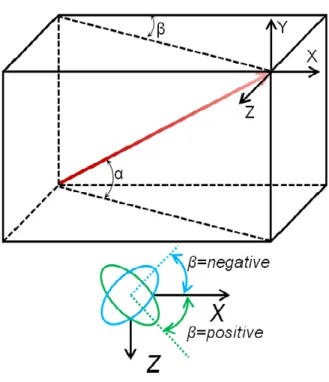
Figure 2: Description of inclination and compound angle with sign convention
Two geometric parameters are discussed here to describe the spacing of film holes within a large array or grid of film holes. The lateral (or transverse) spacing between holes is called the lateral pitch, P. The streamwise (or axial) spacing is known as the streamwise pitch, X. Each spacing is measured from the center of one hole exit area (breakout) to another, whether lateral or streamwise. Both spacing’s are traditionally nondimensionalized by hole diameter, such that comparisons can be made between studies with differing hole diameters. Figure 3 below shows a description of the lateral and transverse spacing’s described.
Figure 3: Description of lateral pitch (P) and streamwise pitch (X)
1.4.2 Independent Parameters Used in Film Cooling
The first film cooling parameter to discuss is the density ratio. The term density ratio signifies the ratio of the secondary flow (coolant) density to that of the primary flow (crossflow), as in Equation 1 . Typically laboratory film cooling studies utilize heated coolant due to
convenience of test setup. Such an action results in an inverted density ratio, where it is common that these studies have a density ratio of less than unity. Although this is opposite from the situation found industrial application, this is a common practice in the experimental research setting. This study uses heated air as the secondary fluid, maintaining an approximate density ratio of 0.8. One noteworthy precaution to take with using air as both the primary and secondary fluid while heating the secondary flow is that conduction effects on the heat transfer surface become significant. Wright et al. [15] investigates this occurrence with several different
measurement techniques, the result being that PSP is the favorable technique to avoid conducting on the heat transfer surface. To minimize this effect, this study utilizes a very low thermal
conductivity material as the heat transfer surface. The characteristics of which will be documented later in this report.
Equation 1: Density Ratio
𝐷𝑅 =
𝜌𝑐𝜌∞
=
𝑇∞
𝑇𝑐
(1)
The next film cooling parameter to discuss is the blowing ratio. The term blowing
ratio signifies the ratio of the secondary flow (coolant) mass flux to the primary flow (crossflow) mass flux, as in Equation 2 . This term accounts for the amount of coolant mass injected for cooling the heat transfer surface, relative to the mainstream flow (or hot gas path). This term involves the relative densities of the fluids, as well as the relative velocities of the fluid streams. Velocity ratio is another common scaling factor used in film cooling, which is absorbed in the blowing ratio for this study.Equation 2: Blowing Ratio
𝑀 = (𝜌𝑈)𝑐
(𝜌𝑈)∞ (2)
The next film cooling parameter to discuss is the momentum flux ratio.
The term momentum flux ratio signifies the ratio of the secondary flow (coolant) momentum flux to the primary flow (crossflow) momentum flux, as in Equation 3. The momentum flux ratio can be determined with knowledge of the density ratio and mass flux ratio. For a given laboratory test at a specified M, the DR dictates the momentum flux ratio of the film cooling jet. The momentum flux ratio is pivotal to the fluid mechanics of the coolant jet, as an increase in momentum yields a tendency for the jet to protrude through the boundary layer on the heat transfer surface, and into the mainstream of the primary flow. This condition of ‘jet lift off’ is often kept in mind when performing film cooling studies, as jet lift off causes a very poor outcome in film coolingeffectiveness over the surface. A non-specific, general case of jet lift off is pictured in Figure 4, to show the different behaviors of film cooling jets in regards to momentum flux ratios.
Goldstein [16] asserts different characteristics of each momentum flux ratio regime. In the first regime, for low momentum flux ratios, Goldstein states that the film cooling effectiveness is increased with increases in coolant mass added. At this point, the thermal inertia of the coolant is utilized fully, and because the film is so attached to the heat transfer surface, the film cooling performance is not regarded to the density ratio of the fluid streams. After an increase in
momentum flux ratio up to a sufficiently high amount, the film cooling effectiveness now depends on the flow properties present (e.g. DR, M, etc.). This regime is described as the mixing regime, and the flow structures / jet lift off now play a more significant role in the effectiveness resulting. Lastly, Goldstein asserts a regime characterized by clear lift off of the coolant jet, off of the heat transfer surface. This regime has complex turbulent structures present, as the turbulent jet penetrates into the turbulent mainstream.
Equation 3: Momentum Flux Ratio
𝐼 = (𝜌𝑈2)𝑐
(𝜌𝑈2)∞=
𝑀2
𝐷𝑅 (3)
1.4.3 Full Coverage Film Cooling
Throughout literature there are a very large number of film cooling studies, each of which may focus on a different quantity or arrangement of holes. Lot of work has been focused on discrete, single film cooling holes. Some of which focus greatly on the governing physics and flow field by using large scale film cooling holes, or even the effect of new, more complex geometries as compared to basic ones (e.g. shaped holes vs. cylindrical holes, etc.). Other studies utilize only a few holes forming a single row, whether it be to investigate the effect of lateral hole spacing on film jet interaction, or any other geometrical configuration. Many correlations and approximations can be found in literature which utilize single row data for conjecturing what the given result of interest (e.g. effectiveness, heat transfer coefficient augmentation, etc.) would be with the subsequent addition of rows of film cooling holes. Such works are also performed for cases with several rows of film cooling holes, to both validate/generate correlations and also directly
measure a given result first hand without the use of correlations. As in the case for this study, only full coverage film cooling arrays are considered in the text matrix. These arrays are composed of many rows of film cooling holes.
Even though there is an extensive amount of literature on film cooling in general, there is a much less complete look at the field of coverage film cooling. A majority of works in full-coverage film cooling are plotted with their case parameters, Figure 5. It is clear that the available literature focuses on relatively small hole spacings, <15D. Also, many studies focus on very simple hole orientations, α=90°, β=0°. The current study focuses on larger spacings, P/D=X/D=23, and angled holes, α=45°, β=-45°, +45°, described in more detail in a following section. Further novelty is achieved through implementing a compound angle shift after 12 rows into the array.
Furthermore, much of the data sets from the studies below are incomplete; they do not present both adiabatic film cooling effectiveness and heat transfer augmentation.
1.4.3.1 Multihole Cooling Film Effectiveness and Heat Transfer [17]
The effect of hole pitch-to-diameter ratio and blowing ratio is studied by determining adiabatic effectiveness and heat transfer augmentation. All the holes are inclined at α=30° and compounded at β=45°. The focus of the study is to provide more information on the influence of hole and row spacing on film cooling array performance. Tests are run at a film-cooling Reynolds number, Re, of 3600, where measurements are taken in a span-averaged manner. The reported uncertainty in heat transfer coefficient is 8%.
Mayle concludes that the integrity of each individual jet can be seen in the adiabatic film-cooling effectiveness. This is universally agreed upon in the current understanding of film
literature. The interaction and coalescence of individual jets is found to have a detrimental impact upon downstream film-cooling effectiveness. Average heat transfer augmentations up to 2.5 are measured, showing that heat transfer augmentation must be considered while designing a film-cooling array.
1.4.3.2 Full-Coverage Film Cooling Part I: Comparison of Heat Transfer Data for Three Injection Angles [18]
Heat transfer experiments are run with α=90°, β=0°, α=30°, β=0°, and α=30°, β=45°. Zero degree inclination angle produces the greatest heat transfer augmentation. Increasing the number of rows increases the downstream recovery region affected area. A compound angled, inclined hole at a mass flux ratio of 0.4 to 0.5 provides the lowest heat transfer augmentation. The highest increase in heat transfer augmentation is seen by normal injection of coolant. An increase in heat transfer augmentation for all geometries is seen at mass flux ratios greater than 0.4. Increasing the number of downstream rows keeps an elevated heat transfer coefficient while increasing the area being protected.
1.4.3.3 Full-Coverage Film Cooling Part I: Comparison of Heat Transfer Data for Three Injection Angles [19]
This study was aimed at characterizing the heat transfer augmentation produced by three film cooling hole orientations; normal injection with no compound angle, inclined at 30° with no compound angle, and finally inclined at 30° with a compound angle of 45°. As expected,
conclusions from the study indicated that heat transfer augmentation was maximized for the normal injection case, and any addition of film cooling rows yielded higher levels of heat transfer in the recovery region. Relevant to this current body of work, comparing the results in heat transfer augmentation for 90° and 45° provides insight into the physical mechanics of the film cooling jets
1.4.3.4 An Investigation of the Heat Transfer for Full Coverage Film Cooling [20]
This study is also a full coverage film cooling study, where ten rows of normally oriented film cooling holes, relative to the heat transfer surface, were tested to investigate the effect of altered levels of freestream turbulence and unheated/heated started lengths prior to the array of film cooling holes. A chief result from this experimental study was that the high and low
turbulence levels in the freestream did not indicate a change in heat transfer augmentation, likely due to the relatively large amount of disturbances and turbulence factored from the film cooling holes injecting in a normal configuration. This result from the study by Kelly and Bogard [19, 20] alleviates concern in the present study of slightly varying turbulence levels effecting heat transfer result.
1.4.3.5 Film Cooling Effectiveness for Injection from Multirow Holes [21]
This is a study investigating the comparison of full coverage array data to predictions of full coverage array data from single row data, and different methods to generate such predictions. The array tested experimentally was comprised of tightly spaced (P/D=3, X/D=5) holes, with compound angle configurations of 45°. The general conclusions were that the traditional
superposition model, and the point source model only performed with reasonable accuracy at sufficiently low blowing ratios (M<0.15), for the tighter lateral and streamwise spacing’s. The test matrix and geometric specimen in this current study exceed the low blowing conditions that were found to be accurately predicted with different models, and thus such models cannot be concluded as applicable directly (without modifications) to this current study.
1.4.3.6 Turbulence intensity effects on film cooling and heat transfer from compound angle holes with particular application to gas turbine blades [22]
This study concludes that the effect freestream turbulence has on film cooling effectiveness and heat transfer is not different for compound angled holes, compared to film cooling holes without compound angles. The effect of freestream turbulence on film cooling effectiveness is most clearly prevalent at off-center locations in the immediate injection region of compounded film holes, where the film experiences significant lateral spreading. Some more well-established links between freestream turbulence and film cooling performance are also validated in the study, such as that the freestream turbulence intensity tends to yield more uniform cooling over the heat transfer surface.
1.4.3.7 Film cooling from two rows of holes with opposite orientation angles: injectant behavior and adiabatic film cooling effectiveness [23]
Ahn, Jung and Lee investigate injectant behavior and adiabatic film cooling effectiveness for two rows of hole with opposite orientation angles. Four configurations are investigated, inline, staggered and two arrangements between the inline and staggered, where z/D=6D, 3D, 1.5D and -1.5D respectively. Inclination angles for all configurations are set to 35°. At lower blowing ratios, the injectant remains attached to the wall, therefore the spatial uniformity is seen to be a larger factor in determining the overall film cooling effectiveness than local film cooling effectiveness level. Increasing blowing ratios to 1.0 and 2.0 increases the interaction between injectant from the
upstream and downstream holes. At higher blowing ratios, inline holes provide higher adiabatic film cooling effectiveness when compared to the staggered configuration. Lower blowing ratios, near M=0.5 provide the highest adiabatic film cooling effectiveness in the near-hole region, where the higher blowing ratios provides better coverage farther downstream.
1.5 Scope and Objective of Current Study
As from the literature survey, the current study utilizes larger lateral and larger
streamwise hole spacings than found in the presented literature survey. Most of the cases from the literature survey presented here are also only considering a large array of film holes with simple hole orientations, as in normal injection without compounding. This study not only investigates arrays with larger hole-to-hole spacings, but also relatively unpopular hole
configurations, such as compound angles of both ±45°. The staggered pattern of positive/negative compound angle in this study also creates yet another unique characteristic in the film cooling arrays which is unique to cases found throughout literature. In regards to the literature surveyed, it is clear that this study proves quite unique from other cases in literature due to large hole spacings within the array (lateral and streamwise), uncommonly large compound angles, and a compound angle shift within the array.
The objective of this work is to consider the test specimen under the test conditions specified in the test matrix, Table 2, and quantify both film cooling effectiveness and heat transfer augmentation for each case.
CHAPTER 2: EXPERIMENTAL SETUP AND TESTING PREPARATION
2.1 Geometries Tested
This chapter describes the physical setup for the experimental tests of film cooling arrays, performed at the Siemens Energy Center, the Center for Advanced Turbomachinery and Energy Research at the University of Central Florida. A detailed description will be provided in this section on the fabrication and configuration of the geometry specimen tested, several technical details of the wind tunnel and crossflow environment, both experimental testing methodologies, and an uncertainty quantification.
2.1.1 Independent Testing Parameters Which Influence Film Cooling
The fundamentals of film cooling necessary to the current study are presented below. In a broad sense, there are geometric parameters and flow parameters which affect film cooling. The hole geometry and orientation have a profound effect on the behavior of the jet leaving the wall. Also, several fluid mechanic parameters dominate the performance once a hole geometry is decided.
Some concepts and parameters discussed in the first chapter will be summarized and repeated here for clarity to those readers who wish for a brief description of test parameters.
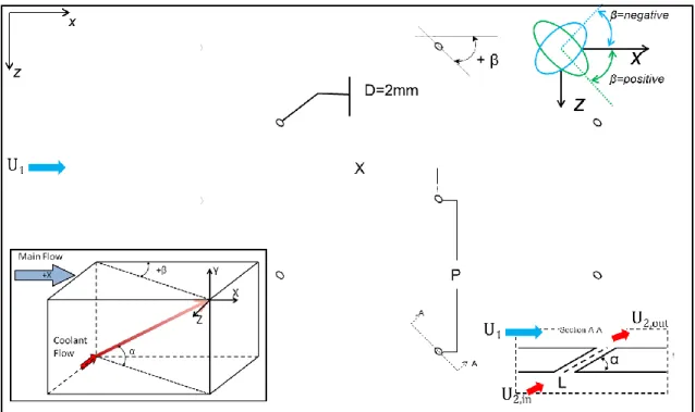
Nomenclature adopted for this body of work describing the cylindrical hole geometry is diagramed in Figure 6. Figure 7 details the geometric parameters describing multiple film cooling holes.
Figure 6: Coordinate system and nomenclature for angles describing film hole geometry
The inclination angle, or surface angle, α is typically between 15-90° for film cooling applications. The effect of α is to adjust the wall normal component of momentum of the coolant jet as it leaves the wall. The compound angle, or flow angle, β can vary anywhere between ±90°. Any deviation from 0° will cause an asymmetric vortex pair exiting the film hole. This is beneficial because it disrupts the induced wall normal velocity, and instead promotes spreading of the jet. The length-scale used for film cooling studies is generally the hole diameter, D. The lateral distance between two adjacent holes, measured from hole exit breakout to adjacent hole exit breakout, is known is the pitch, P. Finally, the stream-wise pitch, X, is the stream-wise distance between two adjacent rows and is normalized to X/D.
β
Main flow
θ
α
X Z YFigure 7: Geometric parameters describing an array of film cooling holes
Figure 8: Geometric parameters describing an array of film cooling holes
Up to this point, the geometric parameters relevant to this body of work which affect the film cooling performance have been briefly discussed. The parameters pertaining to the flow of both the primary and secondary flow are now discussed, for this jet in crossflow situation.
Shown in Equation 4, the blowing ratio (M) describes the ratio of coolant mass flux to mainstream hot gas mass flux. This ratio indicates the amount of mass injected into the boundary layer. Both the mainstream and coolant density (ρ) and average velocity magnitude (U) are used.
Equation 4: Blowing Ratio
𝑀 = (𝜌𝑈)𝑐
(𝜌𝑈)∞ (4)
Other parameters often used to describe film cooling performance are the density ratio (DR) and the momentum flux ratio (I).These are calculated using Equation 5 and Equation 6, respectively. The influence of momentum flux ratio on the dynamics of the jet is shown in Figure 9.
Equation 5: Density Ratio
𝐷𝑅 = 𝜌𝑐
𝜌∞ =
𝑇∞
𝑇𝑐 (5)
Equation 6: Momentum Flux Ratio
𝐼 = (𝜌𝑈2)𝑐
(𝜌𝑈2)∞=
𝑀2
𝐷𝑅 (6)
Figure 9: The general effect of momentum flux ratio, describing lift off
2.1.2 Test Matrix
The focus of the current study is the quantification of local heat transfer augmentation and adiabatic film-cooling effectiveness for two full-coverage film cooling surfaces. All specimen have 22 rows of holes in the streamwise direction. In the lateral direction, all full coverage film cooling rows have a total of 10 holes. All specimens have an L/D of approximately 14 for holes within the regular array. The test matrix can be seen in Table 2.
Table 2: Geometric test speciman matrix for current study
Specimen α (ᵒ) β (ᵒ) X/D P/D Nx
FC.V 45 +45/-45 23 23 12 / 10
2.1.3 Machining Process
The fabrication process for the test geometries began with creating CAD drawings. A CAD drawing for one of the geometries used in heat transfer augmentation testing can be seen in Figure 10. A CNC machine is used to machine all test geometries. Prior to machining the Rohacell plates, several fine grades of sandpaper are used to create a smooth flow side surface. Flanges are machined on the edges of the test section, as in Figure 11, such that the test plate’s surface would be flush with the surface of the wind tunnel. The spindle angle of the CNC machine was altered to vary the end mill’s angle relative to the surface, as in Figure 12. This enabled different inclination angles to be cut, in intervals of 15°. For each spindle orientation, several adapter plates had to be fastened to secure the angle of the cutting axis relative to the test surface. The spindle angle is set with an accuracy of ±0.1°, measured with a standard digital level. Gage blocks with an accuracy of ±40 seconds were also used to verify the hole angles machined. To achieve the desired set of compound angles for the test geometries, a fixture is made to change the orientation of the plate relative to the table. Figure 13 shows the fixture, where slots are made for all compound angles included in the test matrix.
Figure 11: Plates were machined using a CNC
Figure 13: A fixture was made to hold the plates at the appropriate orientation angles (for machining the compounding angle)
After machining, the geometries are measured for uncertainty. Pin gauges are used to check each hole diameter as well as smooth any roughness caused from the milling process. The uncertainty of the pin gauges is 0.0025mm.
Due to the test sections being large, 1.2m in the flow direction, the large test surfaces were broken into streamwise segments for testing. A sample CAD drawing of such breakup of the test section can be seen in Figure 14. These segmented test section pieces were installed into the wind tunnel flush with one another, so that no physical flow trips were present between plates at their transitions. This required great attention to detail when installing the plates, and sometimes required rigid metal tape or wood putty to be placed at the transition.
Figure 14: Test surface composed of three sections (plates)
2.1.4 Geometric Uncertainty
Two different cases are tested for film cooling effectiveness, and one case is tested for heat transfer augmentation. The geometric uncertainty table can be seen in Figure 15, where the uncertainty in each geometry fabricated and tested is listed. A cartoon image for clarity on experimental test setup of the heat transfer surface can be seen in
Figure 16: Experimental setup of heat transfer surface, comprised of three separate plates
2.2 Wind Tunnel
A wind tunnel is designed for the study to accommodate the large (1.2m x 0.55m) test section. This allows for a tunnel tailored for studying large arrays of film holes. The cross-section of the cross flow duct at the test section is 6”x 42”. This corresponds to a height of 73D for the film holes of D=2.06mm. This ensures the dynamics of the jets leaving the film holes are not affected by the duct. The cross section of the tunnel is sized so that the added mass due to injection is insignificant
compared to the main flow; hence, the study is conducted in a nominally zero pressure gradient boundary layer (until pressure insert is put in).
A model of the tunnel is shown in Figure 17. There is a 45cm conditioning section upstream of the test section. There are 2 honeycombs of 1.3cm cell size and L/D=6. There are also 3 screens. These were installed to reduce the turbulence intensity of the main flow. After the conditioning section there is a slight 1-D nozzle with an area ratio of 2 leading up to the test section.
Figure 17: Wind tunnel (crossflow) and plenum (secondary flow) for large film cooling array studies
2.2.1 Blowers
The coolant flow is supplied by an 11kW Spencer Vortex blower capable of 35kPa and 0.3m3/s.
The main flow is driven by a 5kW Ziehl-Abegg fan capable of -1.5kPa and 6.6m3/s. The flow originated
from the blowers is routed to the plenum through PVC piping.
2.2.2 Wind Tunnel Flow Measurements
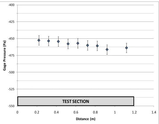
Several static pressure readings are taken along the test section to verify there is not a significant pressure gradient imposed on the flow for tests which do not utilize the pressure gradient wedge. Over the length of the 1.2m test section there is approximately a 15Pa pressure drop corresponding to a -12.5Pa/m favorable pressure gradient. Figure 18 shows the static pressure development in the streamwise direction for zero pressure gradient testing.
Figure 18: Static pressure variation in the stream-wise direction of the duct without the pressure insert in the wind tunnel
The freestream velocity, turbulence intensity, and several other flow measurements are quantified with a constant temperature anemometer (CTA), and displayed in Table 3. Two free stream velocities were tested to provide flow measurements for low and high freestream velocities. This is significant because the freestream velocity will be lowered for several cases involving a significant pressure gradient. The root mean square of the turbulent fluctuations for both freestream velocities is obtained from this data and the turbulence intensity (TI) of the mainstream is quantified at less than 1% for both cases.
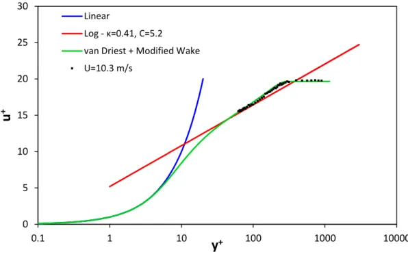
Figure 19 shows the outer scaled velocity profile normalized by the freestream velocity of 27.2 m/s. Similarly, Figure 20 shows the boundary layer thickness for a free-stream velocity of 10.3 m/s. The data was acquired at a rate of 10kHz for 3 seconds per wall normal location. The
-550 -525 -500 -475 -450 -425 -400 0 0.2 0.4 0.6 0.8 1 1.2 1.4 G a ge P re ss u re ( P a ) Distance (m) TEST SECTION