Non-Linear and Unbalanced Three-Phase Load Static Compensation with Asymmetrical and Non Sinusoidal Supply

(1)

Non-Linear and Unbalanced Three-Phase Load Static Compensation with

Asymmetrical and Non Sinusoidal Supply

Reyes S. Herrera1_{and P. Salmerón}1

1_{Electrical Engineering Department}

Escuela Politécnica Superior, University of Huelva

Ctra. Palos de la Frontera, s/n. Palos de la Frontera, Huelva 21819 (España) e-mail: Reyes.Sanchez@die.uhu.es, patricio@uhu.es

Abstract.

P-q theory has been widely used to control active power filters since its formulation in 1983. The compensation strategy used by the p-q theory users has not suffered modification; so it is used the constant power compensation strategy. In this way, the supply instantaneous power after compensation is constant. This kind of compensation strategy has obtained good results in the case of balanced and sinusoidal voltages, however it has not been appropriate in the case of unbalanced or non sinusoidal voltages. In this paper it has been researched about the modifications necessary, into the p-q theory frame, to get control strategies which allow to attack the unit power factor compensation or the balanced and sinusoidal currents compensation.

Keywords.

Instantaneous reactive power, power quality, three-phase systems, harmonics, active power filters.

1. Introduction.

The integration of power electronic in the common life has originated a considerable increase of non linear currents. The problems associated with these currents have made of its compensation a prioritary task. There are several ways to achieve the target (non linear currents compensation), and one of the most used currently is the active power filter (APF). This is a converter which supplies the non useful part of the current required by the load. Imposing a compensation target to the control circuit, it calculates the current supplied by the compensator according to the instantaneous reactive power theory.

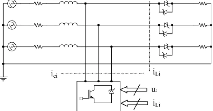
In this paper, the control strategy has been applied to a three-phase four-wire system similar to that presented in figure 1. It is a three-phase balanced and non sinusoidal voltage source. The load involves a regulator composed by bi-directional thyristors and series resistors with different values in each leg to obtain asymmetrical conditions. The compensator inject the non useful part of the current required by the load. Along the paper, lower case represents instantaneous measure, upper case average measure, subindex “L” load requirement, subindex “c” compensator supply and subindex “s” source supply.

From this theory different formulations appeared during the last decade, this work is focused on the first of them, called p-q u original instantaneous reactive power theory.

2. The Original Instantaneous Reactive

Power Theory.

It was formulated at the beginning of the eighties, [1], and this is the formulation which has experimented a largest diffusion along these years. That is the reason to be the most used as control strategy for the APF. The p-q theory was developed to be applied to phase three-wire systems with balanced and sinusoidal source voltages. The compensation target assumed was getting a constant instantaneous source power.

This theory is based on a coordinates transformation from the phase reference system (123) to the 0αβ system, figure 2. The transformation matrixes associated are as follows:

Figure 1. Compensation diagram

ui

iLi

ici iLi

Figure 2. 0αβ reference system

1 2 3 α β 0 3 2 1 120° 120° 120° 0 α β

(2)

























−

=













3 2 1 0

2

3

2

3

0

2

1

2

1

2

1

2

1

2

1

3

2 u

u

e

β α (1)

























−

=













3 2 1 0

2

3

2

3

0

2

1

2

1

2

1

2

1

2

1

3

2 i

i

β α (2)

Looking at these equations it can be deduced that:

3

0 3 2 1

i

_N

=

+

=

(3)

They are defined the different power as follows:

[ ]

          =                     − =           β α β α α β β α αβ αβ i i i P i i i e e 0 e e 0 0 0 e q p p ₀ 0 0 0 0 (4)

where p0 is the zero sequence (real) instantaneous power,

pαβ is the αβ real instantaneous power and qαβ is the

imaginary instantaneous power.

By mean of the [P0] inverse matrix it is possible to

calculate the current components knowing the different power terms. The expression is shown in the next equation:                     − =         αβ αβ α β β α αβ αβ β α q pp e e e e e e e e e e e i ii 0 0 0 0 0 2 2 0 0 0 0 0 0 1 where

e

_αβ2

=

e

_α2

+

e

_β2 (5)

The strategy assumed by this theory since its conception has been the obtention of a constant instantaneous power in the source side with the only restriction of getting a null active power exchanged by the compensator, Pc.

In this way, the first row in the table I shows the control strategy derived from this theory as it was developed originally. In fact, to calculate the compensator current, and according to the figure 1 references, it is verified that:

( )

L

( )

s

( )

L

( )

Lu

c t p t p t p t P

p = − = − (6)

Where PLu is the total active power consumed by the

load. The equation (6) means that:

( )

t p

( )

t P p

( )

t

p_cαβ = _Lαβ − _Lαβ =~_Lαβ (7)

( )

t p

( )

t P p

( )

t

p_c₀ = _L₀ − _L₀ = ~_L₀ (8)

which, effectively, fulfils that < p_c

( )

t >=0, where

( )

t pL

~ _{represents the}_p

_{( )}

_t

L variable part. On the other side,

( )

t q

( )

t

q_c = _L_αβ ₍₉₎

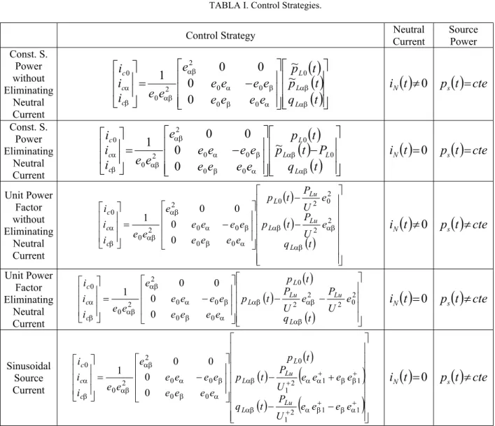
The second column in the table informs whether theory eliminates the neutral current and the fourth one informs about the active power supplied by the source after compensation, saying whether it is constant in time. The strategy shown in the first row does not eliminate the neutral current but the active power exchanged by the compensator is null.

To impose this new restriction, in the p-q theory context, it is only necessary a simple modification: the zero sequence power used to calculate the compensator current is the zero sequence power required by the load, [2]:

( )

t i

( )

t

i_c₀ = _L₀ (10)

( )

t p

( )

t

pc0 = L0 (11)

The third column shows that, effectively, this new strategy eliminates the neutral current. Moreover, the instantaneous power supplied by the source goes on being constant.

3. Other Compensation Strategies.

A compensation strategy widely used along the time is the unit power factor compensation. The target is to get source currents with the same distortion and symmetry conditions as source voltages. It means that the source currents are collinear to the supply voltages. In this situation, the source supplies the load active power, but the instantaneous real power is not constant after compensation, [3].

When source voltages are sinusoidal and balanced, constant power and unity power factor compensations results are the same. In fact, for sinusoidal and balanced source voltages, if compensation currents cancel reactive components, load current distortion and asymmetry, source currents will be sinusoidal and balanced in the same way as voltage. And for that reason, instantaneous power supplied by the source will be constant. However, when supply voltage is unbalanced and non sinusoidal the situation won’t be the same.

The table I third row shows the control strategy, based on the p-q theory, which gets unit power factor in the source side after compensation. Up now it has not been planned this strategy adoption in the p-q theory frame. Now, the source current must be proportional to the voltage supplied:

(3)

e G

ir_s = _er (12)

To go on satisfying that the active power exchanged by the compensator is null, the proportionality constant must be fixed to the next value:

2 U P

G_e = Lu ₍₁₃₎

where U2_≡_E2_{is the square of voltage vector rms value.}

The compensator instantaneous power is the difference between the total real instantaneous power required by the load and the part supplied by the source as it has been explained above. Table I presents the compensator currents equations in 0αβ coordinates.

TABLA I. Control Strategies.

Control Strategy Neutral _Current Source _Power

Const. S. Power without Eliminating Neutral Current

( )

_

























−

=













t

q

t

p

t

p

e

i

L L L c c c αβ αβ α β β α αβ αβ β α

~

0

1

0 0 0 0 0 2 2 0 0

( )

t

≠

0 i

_N

p

_s

( )

t

=

cte

Const. S. Power Eliminating Neutral Current

( )

_













−













−

=













t

q

P

t

p

t

p

e

i

L L L L c c c αβ αβ α β β α αβ αβ β α 0 0 0 0 0 0 2 2 0 0

~

0

1 _{( )}

0 =

t

i

_N

p

_s

( )

t

=

cte

Unit Power Factor without Eliminating Neutral Current

( )

                  − −           − =           t q e U P t p e U P t p e e e e e e e e e e e i i i L Lu L Lu L c c c αβ αβ αβ α β β α αβ αβ β α ₂ 2 2 0 2 0 0 0 0 0 2 2 0 0 0 0 0 0 1

_{( )}

0 ≠

t

i

_N

p

_s

( )

t

≠

cte

Unit Power Factor Eliminating Neutral Current

( )

           − −           − =           t q e U P e U P t p t p e e e e e e e e e e e i i i L Lu Lu L L c c c αβ αβ αβ α β β α αβ αβ β α ₂ 2 ₂ 02 0 0 0 0 0 2 2 0 0 0 0 0 0 1

_{( )}

0 =

t

i

_N

p

_s

( )

t

≠

cte

Sinusoidal Source Current

( )

(

)

( )

(

)

                    − − + −           − =           + + + + + + 1 1 2 1 1 1 2 1 0 0 0 0 0 2 2 0 0 0 0 0 0 1 α β β α αβ β β α α αβ α β β α αβ αβ β α e e e e U P t q e e e e U P t p t p e e e e e e e e e e e i i i Lu L Lu L L c c c

( )

t

=

0 i

_N

p

_s

( )

t

≠

cte

This control strategy does not permit to eliminate the neutral current. To satisfy this restriction, the strategy must be change to the form shown in the table I fourth row. In this case, the power factor is a little lower than the unit. Nevertheless, the neutral current is eliminated even in the case that voltages are not balanced or sinusoidal.

For last years, both compensation objectives presented in this paper are not enough to solve the new problems appeared. It is necessary to define a new compensation target based on an ideal reference case.

Due to the fact that the electrical companies produce, generally, the electrical power as sinusoidal and direct sequence voltages, it has been got as reference condition in the supply. A resistive load, balanced and linear is considered as the ideal reference load. A reference voltage applied to an ideal reference load will generate sinusoidal and balanced currents, in phase with voltages, [4]-[5]. Anything which produces a no conformity with these reference conditions supposes a poor electric power quality. Compensation devices must achieve that the source current are sinusoidal, balanced, on positive sequence and in phase with voltages positive sequence fundamental component. It must be fulfilled for any supply voltages conditions and load kinds. Those

(4)

requirements involve the ideal reference conditions for supply current and they are the currents that define the last compensation objectives assumed in this paper. If voltages are balanced and sinusoidal, ideal currents will be (as in earlier strategy) proportional to the voltages. The proportionality constant must have the value established in the equations (12) and (13), too. If voltages are balanced no sinusoidal, the ideal reference current must be proportional to its fundamental component. The proportionality constant is fixed to satisfy the restriction of having null active power exchanged by the compensator. The ideal current expression is as follows, [6]-[7]: 1 2 1

u

U

P

i

u s

r

₌

(14) 1

u

r

represents the voltage fundamental component and 2

1 2

1 E

U ≡ the square of the voltage fundamental component rms value.

If voltages are unbalanced non sinusoidal, the source current expression becomes as shown in equation (15).

+ +

=

₂ ₁ 1

u

U

P

i

u s

r

₍₁₅₎ + 1

ur represents the voltage positive sequence fundamental

component and 2

1 2 1+ ≡E+

U the square of the voltage positive sequence fundamental component rms value. Now, ir_s in (15) is proportional to the voltage positive sequence fundamental component. The proportionality constant value is got imposing the restriction of null active power exchanged by the compensator as shown in the earlier equation.

In the table I last row it is shown the compensation equations to get balanced and sinusoidal supply currents. They are, as earlier strategies, in 0αβ coordinates. In this case it must be noted that, at first time, it is necessary to impose restrictions not only to the instantaneous real powers p0(t) and pαβ(t), even besides to the instantaneous

imaginary power qαβ(t). This new restriction is necessary

to get sinusoidal and balanced source currents even voltages are non sinusoidal.

Moreover, this strategy achieves to eliminate the neutral current with a null active power exchanged by the compensator.

4. Simulation Practical Results

The five strategies presented in previous items and shown in table I have been applied to the simulation platform shown in figure 1.

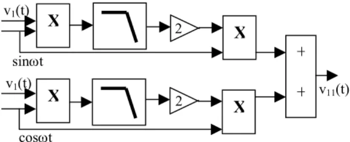
The method used to obtain voltage fundamental component necessary to by the last strategy is based in the use of pass band filters, multipliers and adders as it is shown in figure 3.

The product composed by voltage vector one phase v1(t)

and the signal senωt has a constant term: ½V1cosϕ1 being

V1 the phase 1 voltage fundamental component

amplitude and ϕ1 the phase 1 voltage fundamental

component phase.

On the other hand, the product composed by the same voltage vector v1(t) and the signal cosωt has a constant

term: ½V1sinϕ1. Multiplying both constant terms per 2

and per senωt and cosωt, respectively, as it can be seeing in figure 3, phase 1 voltage fundamental component waveform is built.

To get the other two phases, the procedure may be the same.

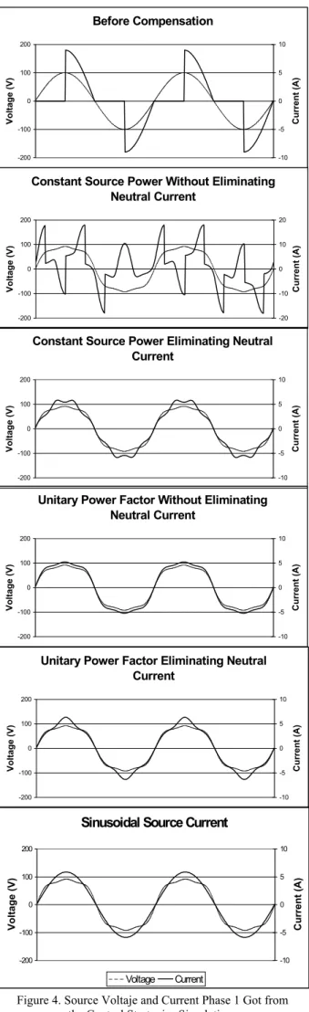
The results got from the different strategies simulations are presented in figure 4. All of them represent the phase 1 source voltage and current waveforms correspondent to the different strategies simulation.

The first graph in figure 4 shows the voltage and current required by the load or the source current before compensation. It is a strongly non linear current load. The second graph presents the current source after compensation according to the first control strategy shown in the table I first row. This strategy looks for getting constant instantaneous power supplied by the source after compensation. The source current is non sinusoidal and it still presents a high distortion. Nevertheless, the third graph shows that, with the only additional restriction of eliminating the neutral current in the same strategy (getting constant the instantaneous power supplied by the source), the current distortion is widely reduced. This second strategy does not get sinusoidal source current as can be seen in the third graph. Both strategies get constant instantaneous power supplied by the source after compensation.

The fourth graph in figure 4 presents the current source after compensation according to the third strategy shown in the table I third row. This is the unit power factor strategy without taking into account the neutral current elimination.

Figure 3. Procedure to get voltage fundamental component

+

X

₂ 2 v1(t) v1(t) sinωt cosωt v11(t)

(5)

In this case, the source current waveform is collinear to voltage. Imposing the additional restriction of eliminating the neutral current, both waveforms (voltage and current) are not collinear. This new strategy is shown in table I fourth row. Nevertheless, the distortion is low in this case, too. Both strategies presented in this paragraph do not get constant instantaneous power supplied by the source after compensation. The power factor is the unit in the fist one and almost the unit in the other.

The current waveform shown in figure 4 sixth graph is the only sinusoidal one. It corresponds to the strategy presented in table I last row, which imposes getting sinusoidal and balanced source currents in phase with the voltages and carrying the active power required by the load. This strategy does not get constant instantaneous power or unit power factor after compensation. However, this is the only case which obtains a source current waveform without any distortion.

5. Conclusion

It has been presented in this paper an exhaustive analysis of the p-q instantaneous reactive power theory. Besides, it has been carried out a new analysis where it is shown that, with few modifications in the control strategy developed by the authors of the original theory, it may be achieve any compensation target imposed to the system. The results are corroborated by the correspondent simulations in the Matlab-Simulink environment.

References

[1]. H. Akagi, Y. Kanazawa, and A. Nabae, “Instantaneous Reactive Power Compensators Comprising Switching Devices Without Energy Storage Components”, IEEE Trans. Ind. App.,vol.IA-20,No.3,pp.625-630, 1984.

[2]. H. Akagi, S. Ogasawara, H. Kim, “The Theory of Instantaneous Power in Three-Phase Four-Wire Systems: A Comprehensive Approach”, Conf.Rec.of IEEE IAC, Vol.1,1999,pp. 431-439.

[3]. A. Cavallini, G. C. Montanari. “Compensation Strategies for Shunt Active-Filter Control”. IEEE Transactions on Power Electronics, Vol. 9, No. 6, November 1994, pp. 587-593. [4].P. Salmerón Revuelta, R. S. Herrera, “Application of the Instantaneous Power Theories in Load Compensation with Active Power Filters”, EPE 2003.

[5]. Fang Z. Peng, Leon M. Tolbert, “Compensation of Non-Active Current in Power Systems –Definitions from Compensation Standpoint”-, Power Enginnering Society Summer Meeting, 2000, Volumen: 2, 2000, pp 983-987.

[6]. P. Salmerón, J.C. Montaño, J. R. Vázquez, J. Prieto and “A. Pérez, Practical Application of the Instantaneous Power Theory in the Compensation of Four-Wire Three-Phase Systems”, IECON’02, Sevilla, 2002, Volumen 4, pp 650-655.

[7]. P. Salmeron, J.C. Montaño, J.R. Vázquez, J. Prieto and A. Pérez, “Compensation in Non-Sinusoidal, Unbalanced Three-Phase Four-Wire Systems with Active Power Line Conditioner”, IEEE Trans on Power Delivery, in press.

[8]. A. Horn, L. A. Pittorino, J. H: R. Enslin, “Evaluation of Active Power Filter Control Algorithms Under Non-Sinusoidal and Unbalanced Conditions”, Proc. of the 7th International conference on Harmonics and Quality of Power, ICHQP 1996, pp 217-224.

[9]. H. Kim, Hirofumi Akagi, “The Instantaneous Power Theory on the Rotating p-q-r Reference Frames”, PEDS’99. Figure 4. Source Voltaje and Current Phase 1 Got from

the Control Strategies Simulations

Constant Source Power Without Eliminating Neutral Current -200 -100 0 100 200 Voltage (V) -20 -10 0 10 20 Current (A)

Constant Source Power Eliminating Neutral Current -200 -100 0 100 200 Voltage (V) -10 -5 0 5 10 Current (A) Before Compensation -200 -100 0 100 200 Voltage (V) -10 -5 0 5 10 Current (A)

Unitary Power Factor Without Eliminating Neutral Current -200 -100 0 100 200 Voltage (V) -10 -5 0 5 10 Current (A)

Unitary Power Factor Eliminating Neutral Current -200 -100 0 100 200 Voltage (V) -10 -5 0 5 10 Current (A)

Sinusoidal Source Current

-200 -100 0 100 200 Voltage (V) -10 -5 0 5 10 Current (A) Voltage Current

(6)

[10]. A. Gosh and A. Joshi, “A new approach to load balancing and power factor correction in power distribution system”, Power Delivery, IEEE Transactions on, Volume: 15, Issue: 1, Jan. 2000, pp. 417–422.

[11]. M.C. Ben habib, E. Jacquot, S. Saadate, “An advanced Control Approach for a Shunt Active Power Filter” ,

ICREPQ’03, Vigo, 2003.

[12]. M. Depenbrock, V. Staudt and H. Wrede, “A Concise Assesment of Original and Modified Instantaneous Power Theory Applied to Four-Wire Systems”, PCC, 2002, Proc of the vol 1, pp: 60-67.