Integrating Stream Parallelism and Task
Parallelism in a Dataflow Programming Model
by
Drago§ Dumitru Sbirlea
A
THESIS SUBMITTEDIN PARTIAL FULFILLMENT OF THE REQUIREMENTS FOR THE DEGREE
Master of Science
APPROVED, THESIS COMMITTEE:
Vivek Sarkar
Professor of Computer Science E.D. Butcher Chair in Engineering
L. John and Ann H. Doerr Professor of Computational Engineering
~-~
Associate Professor of Electrical and Computer Engineering
Jun Shirako Research Scientist
Computer Science Department
Houston, Texas
Integrating Stream Parallelism and Task Parallelism in a Dataflow Programming Model
by
Drago§ Dumitru Sbirlea
As multicore computing becomes the norm, exploiting parallelism in applications becomes a requirement for all software. Many applications exhibit different kinds of parallelism, but most parallel programming languages are biased towards a specific paradigm, of which two common ones are task and streaming parallelism. This results in a dilemma for programmers who would prefer to use the same language to exploit different paradigms for different applications. Our thesis is an integration of stream-parallel and task-stream-parallel paradigms can be achieved in a single language with high programmability and high resource efficiency, when a general dataflow programming model is used as the foundation.
The dataflow model used in this thesis is Intel's Concurrent Collections (CnC). While CnC is general enough to express both task-parallel and stream-parallel paradigms, all current implementations of CnC use task-based runtime systems that do not de-liver the resource efficiency expected from stream-parallel programs. For streaming programs, this use of a task-based runtime system is wasteful of computing cycles and makes memory management more difficult than it needs to be.
We propose Streaming Concurrent Collections (SCnC), a streaming system that can execute a subset of applications supported by Concurrent Collections, a general
allows application developers to benefit from the efficiency of stream parallelism as well as the generality of task parallelism, all in the context of an easy-to-use and general dataflow programming model.
To achieve this integration, we formally define streaming access patterns that, if respected, allow CnC task based applications to be executed using the streaming model. We specify conditions under which an application can run safely, meaning with identical result and without deadlocks using the streaming runtime. A static analysis that verifies if an application respects these patterns is proposed and we describe algorithmic transformations to bring a larger set of CnC applications to a form that can be run using the streaming runtime.
To take advantage of dynamic parallelism opportunities inside streaming applica-tions, we propose a simple tuning annotation for streaming applicaapplica-tions, that have traditionally been considered with fixed parallelism. Our dynamic parallelism con-struct, the dynamic splitter, which allows fission of stateful filters with little guidance from the programmer is based on the idea of different places where computations are distributed.
Finally, performance results show that transitioning from the task parallel runtime to streaming runtime leads to a throughput increase of up to 40x.
In summary, this thesis shows that stream-parallel and task-parallel paradigms can be integrated in a single language when a dataflow model is used as the foundation, and that this integration can be achieved with high programmability and high resource efficiency. Integration of these models allows application developers to benefit from the efficiency of stream parallelism as well as the generality of task parallelism, all in the context of an easy-to-use dataflow programming model.
I would like to thank my advisor, Professor Vivek Sarkar, for his guidance during my graduate studies. His advice has always been insightful and realistic and helped keep this work on track. His management skills insured that non-research related problems did not cause delays. I am also grateful to him for the opportunity of working in such a wonderful group as the Habanera team.
I express my appreciation for my committee members: Prof. Keith D. Cooper, Prof. Lin Zhong and Jun Shirako, their careers have served as models and inspiration for my approach to research.
Jun Shirako has been always willing to help; it has been a pleasure to work with him on both personal and professional level.
My fellow graduate students from the Habanera group have enriched my research experience. Great ideas are born from interaction and I appreciate the discussions I had with all of them. I owe a lot of thanks to Sagnak Tasirlar who guided me through the tools used in this work.
Last but definitely not least, without my wife's support and patience this thesis would never have been possible.
Abstract Acknowledgments List of Illustrations List of Tables
1 Introduction
2 Previous Work
2.1 Streaming Languages .2.2 The Concurrent Collections Model 2.3 Habanero Java
2.4 Phasers . . . .
2.5 Phaser accumulators and streaming phasers
ii iv viii X
1
4
4 8 11 12 143 Streaming extensions for Concurrent Collections
16
3.1 Streaming CnC . . . 16
3.2 Well-formed Streaming CnC graphs 16
3.3 Comparing SCnC to streaming and to CnC . 18
3.4 Step-local collections . . . 22
3.5 Dynamic Parallelism support 23
4 Towards automatic conversion of Macro-dataflow
Pro-grams to Streaming ProPro-grams
4.1 Transforming a CnC graph to a well formed shape .
25
274.1.1 Possibility and Profitability of a CnC to SCnC transformation 27 4.1.2 Algorithm for converting a CnC graph to well formed shape 28 4.1.3 Algorithm analysis . . . 34 4.2 Identifying streaming patterns in a well formed CnC graph
4.3 Deadlock . . . . 4.4 Deadlock freedom .
4.5 Converting CnC tags to Streaming CnC tags .
5 Efficient Implementation of SCnC
5.1 Use of streaming phasers . . . . 5.2 Implementation of Dynamic Parallelism .6 Results
6.1 Implementation status 6.2 Testing methodology 6.3 Applications . . . . 6.3.1 FilterBank . 6.3.2 BeamFormer . 6.3.3 FMRadio . .6.3.4 Facility Location without dynamic parallelism 6.3.5 Facility Location with dynamic parallelism . . 6.3.6 Sieve of Eratosthenes with dynamic parallelism
7 Related work
8 Conclusion and future work
8.1 Conclusion . . 8.2 Future Work . 35 43 45 4749
49 5463
63 63 65 65 66 70 71 74 7479
84
84 843.1 A CnC Step-local item collection with its corresponding step collection 22
4.1 The workflow of converting a CnC application to Streaming CnC . . 26 4.2 Conversion of environment from multiple producer to single producer
by adding an additional step . . . 29 4.3 Conversion of a control collection with multiple prescribed step
collections to a control collections that prescribes a single step collection 30 4.4 Conversion of a collection with multiple producers to a collection
with a single producer . . . 32 4.5 Conversion of a collection from multiple consumers to a collection
with a single consumer . . . 33 4.6 The SCnC graph for the 2 branches of the Filter Bank application,
annotated with item-put, item-get and tag-put and tag-get functions
(after step 5 of the algorithm) . . . 38 4. 7 The SCnC graph for the 2 branches of the Filter Bank application,
annotated with producer and consumer functions for item collections, after applying the algorithm . . . 39
5.1 The Streaming CnC graph with dynamic parallelism: step S1 and 81' correspond to a single step collection, 81 processing the class of tags
5.2 The Streaming CnC dynamically parallel execution of a step that consumes one item and produces one item. The item is produced only after both places have signaled, but parallelism can still be exploited in this situation.
6.1 The workflow for using a CnC application for SCnC. The only
58
manual transformations are marked with a star, the rest are automatic. 64 6.2 The SCnC graph for the FilterBank application is identical for SCnC 66 6.3 The CnC graph for BeamFormer application . . . .
6.4 The StreamingCnC graph for BeamFormer application 6.5 The dynamic StreamingCnC graph for Sieve application.
6.6 The dynamic StreamingCnC graph for Sieve application pipeline version.
68
69
762.1 Types of edges in a CnC graph . . . 10
3.1 Mapping between CnC concepts and streaming concepts . . . 19 3.2 Comparison between CnC and SCnC: the number of producers and
consumers supported by different building blocks . . . 19 3.3 Comparison between Streaming and Streaming CnC: number of
producers and consumers supported by different building blocks 20 3.4 Comparison between Streaming and Streaming CnC: number of input
and output streams for a step . . . 20 3.5 Comparison between Streaming and Streaming CnC item get semantics 21
6.1 SCnC, CnC and streaming phasers performance for FilterBank (Core i5) 67 6.2 SCnC, CnC and streaming phasers performance for FilterBank (Xeon) 67 6.3 SCnC, CnC and streaming phasers performance for Beamformer (Xeon) 70 6.4 SCnC, CnC and streaming phasers performance for Beamformer
(Core i5) . . . 70 6.5 SCnC, CnC and streaming phasers performance for FMRadio (Xeon) 71 6.6 SCnC, CnC and streaming phasers performance for Facility Location
(Core i5 system) . . . 73 6. 7 SCnC, CnC and streaming phasers performance for Facility Location
6.8 SCnC dynamic parallelism execution time, compared to the SCnC implementation, 16 core Xeon . . . . 6.9 SCnC dynamic parallelism execution time compared to SCnC
75
Chapter 1
Introduction
As modern processors hit the power and frequency walls, multicore architectures are the solution to allow future processors to continue scaling. For the software developer to take advantage of the new various types of processing power available, new programming models are needed, that can the express the multiple types of parallelism that an application might have.
Two common paradigms for parallelism are task parallelism and stream paral-lelism. There is a large family of task-parallel programming languages and libraries currently available including OpenMP 3.0[1], Java Concurrency, Intel Threading Building Blocks[2], .Net Parallel Extensions[3], Cilk[4], and Habanero-Java[5]. Like-wise, a number of stream-parallel programming languages have been proposed in the past, with Streamit[6] being the most recent exemplar for the stream-parallel paradigm.
Applications for the streaming paradigm are common and becoming more and more prevalent. Up to 37% of Internet traffic is done by streaming video and have been estimated to take up to 90% of compute cycles as early as 2000s[7]. DSP ap-plications, cell phone network call processing, database and classification algorithms, media streaming, HDTV video and audio processing and other compute-intensive applications are candidates for efficient parallel implementation using streaming lan-guages. However, the expressiveness of streaming languages and programming models is usually limited to streaming parallelism and they are unable to express other forms
of parallelism easily.
Macro dataflow programming languages such as the Intel Concurrent Collections ( CnC) [8] are well suited for multicore execution of tasks because they separate the definition of the tasks from their scheduling, thereby making exploitation of different types of parallelism easier. The current CnC implementations only take advantage of the task based parallelism, like many other parallel programming models. As a result, the performance of applications following the streaming parallelism patterns suffers greatly if written in standard CnC. Integration of the two models would provide the best of both worlds: the generality and ease of use of task-based programming models, together with the performance streaming can offer to particular kinds of applications. The Streaming CnC extensions introduced in this thesis bring the benefits of stream-ing parallelism with some of the flexibility of task based parallelism through a dynamic split-join parallel construct; this construct allows dynamic creation of streaming filters in certain situations, bringing the parallelism to higher values to potentially match the parallelism of the machine.
Many previous streaming languages or frameworks do not offer either determinism or deadlock-freedom guarantees. This work preserves the determinism guarantees of CnC and provides an algorithm that can statically adjust the size of the buffers to ensure a deadlock equivalence between the streaming and task based execution: no extra deadlocks can happen with streaming compared to task based and if task based is deadlock free, so is the streaming execution.
The structure of the thesis is as follows. Chapter 2 looks at previous work on which this thesis builds, including streaming languages, the Concurrent Collections language and the Habanero Java language which is used to build both the task based and streaming runtime proposed. Chapter 3 describes the design and features of
Streaming CnC, the CnC subset that can be run using the streaming runtime. It describes interesting patterns that can be streaming-optimized and shows the dynamic parallelism feature that we propose. Chapter 4 describes how we can identify through analysis if an application conforms to the streaming restrictions and how we can obtain deadlock freedom guarantees if this is the case.
Chapter 5 and 6 describe the implementation of the streaming runtime and the performance results obtained on the set of benchmarks. In Chapter 7 we discuss and compare the related works and we conclude in Chapter 8 with future work directions.
4
Chapter 2
Previous Work
This work builds on past work on streaming languages (Section 2.1) and Habanera Concurrent Collections(Section 2.2), Habanera Java (Section 2.3), phasers, accumula-tors and streaming phasers (Sections 2.4 and 2.5). Streaming Concurrent Collections, the streaming system proposed in this thesis is related to streaming languages; as a notable example of such languages, Streamlt, has provided a rich source of streaming applications to test our work on.
2.1
Streaming Languages
Streaming parallelism is a type of parallelism encountered for applications that work over data that is structured as a "stream" . Characteristics of such applications have been suggested [6], and the most important are:
• Processing large streams of data. The application has to execute operations on a large dataset, viewed
as
a sequence of data items that might not have a specific end point (unbounded size). However, each item must have a limited lifetime.• Stream filters process the input sequence through specific operations that allow reading input items from the input stream and producing items to an out-put stream. The filters are connected to each other through the streams they process: the output stream of one filter can be the input to another, thereby
forming the streaming graph. Filters are relatively independent with few com-munications between them outside of the streams.
• The streaming graph structure does not change often.
The Streamit language was designed to better express and take advantage of the structure of these applications. The original paper [6) allowed for static flow rates through single input and single output filters with special split and join nodes. It supported three main constructs that, combined, could allow concise descriptions of stream applications: the pipeline, split-join and feedback loop patterns. Listing 2.1 shows a Streamit pipeline with 3 filters (lines 20-22), one of which is a finite impulse response filter (FIR Filter), defined through a class with an initialization function (lines 4-9) and a work function (lines 10-17). The processing of the filter is done in the work function, but the initialization is needed to set members to their initial values and also describe the type of data items contained by the stream.
1 class FIRFilter extends Filter {
2 float[] weights;
3 int N;
4 void in it (float[] weights) {
s setinput (Float. TYPE); setOut put (Float. TYPE);
s set Push (N) ; set Pop ( 1) ; set Peek (N) ;
7 this.weights =weights;
s this .N = weights .length;
9 }
10 void work () {
11 float sum = 0;
12 for ( int i =0; i<N; i++)
13 sum -t= input. peek ( i) *weights [ i } ;
6
15 output. push (sum);
16 } 17 }
18 class Main extends Pipeline {
19 void init () {
20 add (new DataSource () ) ;
21 add(new FIRFilter(N));
22 add(new Display());
23 } 24 }
Listing 2.1: Example of a Streamit filter and its use when building a simple pipeline based application
An example of connecting filters using split and join nodes is shown in Listing 2.2. The filter presented consists of a splitter node that duplicates its input so that each child branch gets the same items (line 3) followed by a delay on each of the two branches (lines 4 and 5). The two delay filters feed into a join filter that takes input alternatively from the two branches (line 6). Together, the round robin join and delays with different amounts create an echo effect.
1 class EchoEffect extends SplitJoin {
2 void init () {
3 set Splitter (Duplicate());
4 add (new Delay (100));
5 add(new Delay(O));
6 setJoiner (RoundRobin());
7 }
8 }
Listing 2.3 shows the use of the feedback loop pattern in building a Fibonacci string. The filter result stream is duplicated (line 15) after computing the sum of the previous values(line 12) and the value fed to its round robin join node that outputs only items from the feedback loop: 0 from the the normal edge, 1 from feedback (line 4).
1 class Fibonacci extends FeedbackLoop { 2 void init () { 3 setDelay (2); 4 setJoiner (RoundRobin(O ,1)); 5 setBody(new Filter() { 6 void init () { 7 setlnput(Integer.TYPE);
8 setOutput (Integer .TYPE);
9 set Push ( 1) ; setPop ( 1) ; set Peek ( 2) ;
10 }
n void work() {
12 output. push (input . peek ( 0 )+input. peek ( 1)) ;
13 input. pop() ;
14 }} ) ;
15 s e t S p 1 i t t e r ( D up li cat e () ) ; 16 }
17
18 int initPath(int index) {
u return index; 20 }
21 }
2.2 The Concurrent Collections Model
The Concurrent Collections(CnC) programming model[8] is a macro dataflow parallel programming system that uses components of three types to model programs: item collections, control collections and step collections. These collections and their rela-tionship are defined statically for each application in a CnC specification file and the code of the application, split in tasks-like steps, can be written in any one of multiple languages for which there is a CnC runtime available.
Step collections are procedures in today's programming languages. Control col-lections drive the control flow of the program, by executing a procedure corresponding to a step collection when a control tag is "put" in the control collection(prescribed). The task that is executed is called step instance and receives the control tag as pa-rameter. The step instance can then cause other step instances to run by putting new control tags in control collections.
Item collections play the role of variables in other programming languages and are sets of key-value pairs. Each item represents a value, which is put in an item collection with an assigned tag once during the execution of a program, respecting a single assignment rule. The tag can later be used to access that item (by the same step, or by another). The only restriction is that the step has to be registered as a producer on the control or item collection to which it puts tags.
Tag collections, also called control collections are the data that characterize the control flow of a step. A put into a tag collection leads to a step instance being prescribed. A prescribed step can start executing, but cannot finish executing until the items it reads become available through put operations performed by other step instances.
item, control and step collections in a CnC application. It is used by the runtime to ensure the access of the steps to the correct values in item collections, the execution of the correct steps when a tag is put into a control collection; the graph is also useful for the programmer, as an execution model that shifts the complexity of synchronization and communication between tasks from the programmer to the system,
The CnC graph is a directed graph whose nodes belong to the union of envi-ronment node, item, tag and step collections and edges consist of item-put edges (source: step, destination: item collection) representing producer relationship, item-get (source: item collection, destination: step) representing consumer relationship, tag-put (source: step, destination: control collection) representing control relation-ship, prescription edges (source : control colleCtion, destination: step collection) and environment edges (from the environment node).
In this work, the following restrictions are implied for a CnC graph to be valid:
1. At least one tag collection is produced by the environment (There is at least an edge X-
>
T where X is the environment node and T a control collection).2. For each step collection , there is at least a possible execution that contains the execution of a step instance in that step collection.
Definition 2.1 The CnC control graph is the CnC subgraph restricted to only the environment node and control collections and step collections nodes and the tag-put and prescription edges.
Theorem 2.1
Tbere is a patb in tbe CnC control grapb from tbe environment to any step collection. Proof 2.1 Proof by contradiction. Presume there is a step collection SCO for which there no path from the environment. According to the second restriction stated above,
10
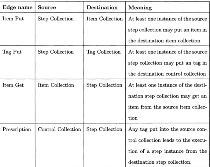
Edge name Source Destination Meaning
Item Put Step Collection Item Collection At least one instance of the source step collection may put an item in the destination item collection Tag Put Step Collection Tag Collection At least one instance of the source
step collection may put an tag in the destination control collection Item Get Item Collection Step Collection At least one instance of the desti-nation step collection may get an item from the source item collec-tion
Prescription Control Collection Step Collection Any tag put into the source con-trol collection leads to the execu-tion of a step instance from the destination step collection.
11
at least one step instance from that step collection has to be able to execute. For this to take place, there has to be another step collection SC1 that produces tags to execute steps in SCO and has a path from the environment, so that it is executable. Thus, we discovered the path Env -+ ... -+ SC1 -+ SCO, which contradicts our hypothesis. D
Theorem 2.2
The CnC control graph is weakly connected.
Proof 2.2 A directed graph is weakly connected if by replacing all its directed edges with undirected ones, the resulting (undirected) graph is connected. Proof by con-tradiction. I presume there is a step collection V and there is no path from it to another step collection T. But we know from Theorem 2.1 that for any node there is a path to the environment. For step collection V, this path would be: Env-+ N1-+ N2-+ .... -+ V and forT, the path is: Env-+ M1-+ M2-+ ... -+ T. Thus, if we consider an undirected graph, V and T must be connected via Env, which contradicts our hypothesis. D
2.3 Habanero Java
The Habanero Java (HJ) [9] language is a programming language derived from XlO and developed in the Habanero Multicore research group which offers primitives for productive parallel programming. The base unit for parallel programming are tasks called asyncs, that are accompanied by a finish termination construct. Habanero Java supports a superset of Cilk's [10] spawn-sync parallelism. It eliminates the Cilk requirement that parallel computations should be fully strict: in HJ, join edges don't have to go to the parent in the spawn tree [11].
2.4 Phasers
Phasers [12] are Habanero Java synchronization constructs that unify for point to point and collective synchronization for a dynamically variable number of tasks. The phaser registration mode models the type of synchronization required: signal-only and wait-only modes for producer and consumer synchronization patterns and signal-wait for barrier synchronization. In our work, we mainly use the producer consumer synchronization and only use collective synchronization (barriers) for the dynamic parallelism feature.
The Habanero Java implementation of phasers works by registering the phaser in the desired mode to each async that will use it. For the purposes of this work, one async will be the producer and one the consumer, so the code looks as shown in Listing 2.4. The producer task (line 5-8) creates an item (line 7) and then signals (line 9) the consumer task. The consumer task can then proceed past the wait call in line 15 on the same phaser used by the producer for signalling. Notice the phaser registrations that accompany the task creations(lines 6 and 13): signal mode for the producer and wait mode for the consumer.
An important detail is that this use of phasers - with explicit wait and signal operations - is, in general, not deadlock free. This desirable properly is offered by only using special next operations. Next operations are expanded to a sequence of signal and wait and in the absence of other signal and wait operations cannot deadlock [12] . Our choice of having multiple input streams per filter meant we have to wait for a variable number of times on each phaser, which is incompatible with the next operation.
The choice of using phasers for synchronization in this work was also supported by their ability of accommodate a dynamically varying number of tasks, unlike normal
barriers. Their particular speed obtained by busy waiting in certain specific scenarios and have proved very efficient on current multicore processors.
2 final Item item= new ProducerConsumerltem();
3
I I
phaser declared with both signal and wait capabilities4 final phaser phl =new phaser(phaserMode.SIG_WAIT);
5
6
I I
the producer task is registered in signal mode 7 async phased ( phl <phaser Mode . SIG >) {8 item. produce() ;
9
I I
signal mode registration allows the signal operation10 phl. signal();
11 }
12
13
I I
and the consumer in wait mode 14 async phased ( phl <phaser Mode . WAIT'>) {15
I I
wait mode enables the call to phaser. wait16 phl. wait();
17
I I
the consumer is blocked at the wait call18
I I
until the signaller performs the signal operation19 item. consumer();
20 }
2.5 Phaser accumulators and streaming phasers
Phaser accumulators [13] are a reduction construct built over the synchronization capabilities of Habanera phasers. Each producer (which is registered in signal mode) sends a value to be reduced in the current phase and then, when all producers have signalled to the phaser, the consumer (which is registered in wait mode) can be unblocked and use the reduced value, as shown in Listing 2.5. An accumulator is associated with a phaser (ph) and needs to know the type of the values it is reducing (int) and what is the reduction operation (SUM). The consumers can send their values and then signal the phaser. The producer will get unblocked from its wait call after all signals have been received and it can access the reduced value through the accumulator result call.
1 final phaser phl =new phaser(phaserMode.SIG_WAIT);
2 accumulator ace =new accumulator(ph, int. class, SUM);
a
I I
multiple producers which reduce their produce values4 for ( int i =0; i< N; i++)
s async phased (phl<phaserMode.SIG>) {
s in t val = produce() ;
1 ace . send (val) ;
s phl. signal() ;
9 } 10
11 async phased (phl<phaserMode. WAlT>) {
12 phl.wait();
1a int reducedValue ace. result();
14 }
We use an extension of accumulators and phasers that is useful for streaming, called bounded phasers or phaser beams [14]. This extension eases the use of these constructs for streaming programs by adding support for bounded buffer synchronization in phasers and accumulators.
A bounded phaser is created with a given bound, k. In our work the bound is 1000. For phasers, the producer can proceed at most k phases ahead of the consumer. A bounded accumulator contains an internal circular buffer whose size matches the bound k that is used to store the additional items before they are consumed. Access to previously consumed elements is permitted, in the limits of the internal buffer, by providing an additional parameter to the result() call. The parameter is used as an offset from the current position in the buffer. These primitives provide the means for implementing our streaming runtime.
Chapter 3
Streaming extensions for Concurrent Collections
3.1 Streaming CnC
In this chapter, we introduce Streaming CnC (SCnC) as a subset of the CnC model (graph specifications, corresponding code generator and runtime library) that al-lows implementation and runtime support for building CnC applications that exploit streaming parallelism as opposed to task parallelism.
To make this possible, we need a mapping between CnC concepts and streaming concepts.We identified this mapping and it is shown in table 3.1. A subset of the CnC graphs where this mapping is valid and can be implemented efficiently has to be found. Theoretical characterization of this subset is presented in section 3.2 and the engineering considerations behind our choice is presented in section 5.1. A comparison between CnC, its SCnC subset and streaming graph shapes can be found in Section 3.3.
3.2 Well-formed Streaming CnC graphs
Only a subset of the graphs that are legal CnC graphs can be used as input for SCnC. This is because of the nature of streaming (not any application is a stream-ing application) and because of implementation considerations (underlystream-ing phaser beams reduction restriction). This section describes this subset in detail, but does not describe the restrictions on what item gets and puts are legal in SCnC.
The conceptual requirement on the shape of the CnC graph is that the CnC graph is well formed and its the CnC control graph is a directed tree. The analysis of the shape of this graph will prove useful when we try and formalize the requirements of streaming applications, specifically when we loop at streaming access patterns.
Definition A well formed CnC graph respects the following conditions:
1. Control collections have only one producing step collection and one prescribed step collection.
2. Item collections have only one producing and one consuming step collections.
3. The environment only puts tags into a single tag collection and has no other put edge (to any other tag or item collection). This tag collection whose tags are supplied by the environment is the root of the tree and has a single child, the entry step of the graph.
The data is provided through the control tags that get put from the environment; each tag can store also a data point of the stream.
Theorem 3.1
The CnC control graph of a well formed graph is a directed tree.
Proof 3.1 A directed tree is a directed graph with no cycles. We know from Th 2.2 the CnC control graph is weakly connected, need to prove the absence of cycles. As both step and tag collections have only one predecessor and at the same time the environment has none and it is connected to all nodes, this conclusion is obvious. No cycles and weak connectivity limply the desired conclusion. D
The root of the CnC control graph could be considered to be the environment. For uniformity, as the environment is not a standard step and because it is restricted
to a single child, we can consider the root of the tree to be the sole child of the environment: the control collection of the entry node .
Theorem 3.2
The CnC control graph with the entry control collection as its root is an arborescence. An arborescence is a directed, rooted tree in which all edges point away from the root. The CnC control graph with entry control collection as root is a directed tree, as Theorem 3.1 showed. We know that there is a directed path from the environment to each step collection (Theorem 2.1). As the entry control collection is the singular child of the environment all paths pass through it, so there must be a path from the entry control collection to every node.
The paths starting from the root start from tag collection and end in control collections, which is the correct orientation of the prescription edges in the CnC control graph, or they might go from step collection to tag collection, which is the correct orientation for control put edges. There is no other type of edges in the control graph.
3.3 Comparing SCnC to streaming and to CnC
The design of Streaming CnC started from the observation that some CnC concepts map naturally to streaming concepts: item collections can be viewed as streaming queues and steps as filters. Of course, there are differences such as the explicit control flow in CnC and the formalization of the environment. The mapping between streaming constructs and SCnC constructs is in table 3.1
Control collections support just a subset of the item collections operations ("put last" and "get first" instead of "put anywhere" and "get from anywhere"). The restriction on their operations compared to item collections comes from the fact that
CnC name Streaming name I tern collection Queue between filters
Control collection No exact match in streaming as control flow is not explicit. Step collection Filter
Environment Not formalized (input stream)
Table 3.1 : Mapping between CnC concepts and streaming concepts
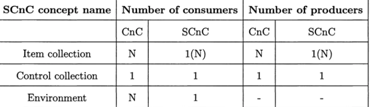
SCnC concept name Number of consumers Number of producers
CnC SCnC CnC SCnC
Item collection N l(N) N 1(N)
Control collection 1 1 1 1
Environment N 1 -
-Table 3.2 : Comparison between CnC and SCnC: the number of producers and con-sumers supported by different building blocks
in streaming applications there is a specific order in which the filters process data: the order in which the items are put. Realizing that control collections for streaming applications are in fact queues too queues,we mapped hem to the same primitives as item collections which are item queues.
A comparison of the number of producer / consumer edges supported by the different component types of SCnC and streaming and CnC is found in tables 3.2 and 3.3. Note that the number of consumers and producers of item collections is limited to 1 in SCnC. The restriction on multiple consumers of an item collection relaxed for dynamic parallelism; there, the consumers are "synchronized" consuming the same items in the same order and and are prescribed the same number of times.
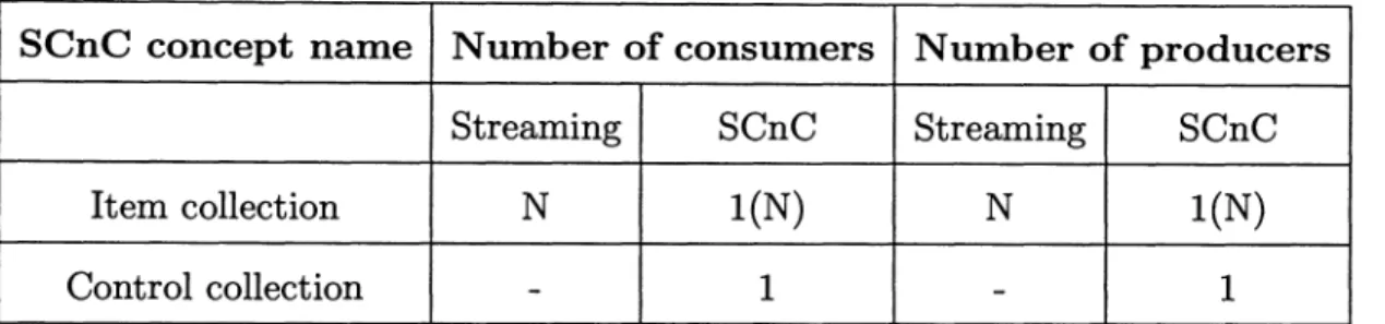
SCnC concept name Number of consumers Number of producers
Streaming SCnC Streaming SCnC
Item collection N 1(N) N 1(N)
Control collection
-
1-
1Table 3.3 : Comparison between Streaming and Streaming CnC: number of producers and consumers supported by different building blocks
SCnC concept name Number of consumers Number of producers
Streaming SCnC Streaming SCnC
Step collection 1 N 1 N
Table 3.4 : Comparison between Streaming and Streaming CnC: number of input and output streams for a step
The single consumer restriction for item collections does not necessarily decrease the number of programs that can be expressed, it just makes the distributions/du-plications explicit in the SCnC graphs by split and join nodes. Distribution and collection (join operation) - the patterns of communication affected by the change - are actually operations themselves, it is natural for them to be explicit in a CnC based model. These operations are discussed in detail in Section 4.1.
Having join operations as explicit steps helps solve the determinism problems that might happen in a multiple producer/consumer scenarios otherwise, because the join step explicitly states the order of the gets and puts. Furthermore, a single SCnC step can operate on a number of inputs and output collections larger than one, as opposed to the limitation of Streamlt to a single input and output, as seen in Table 3.4.
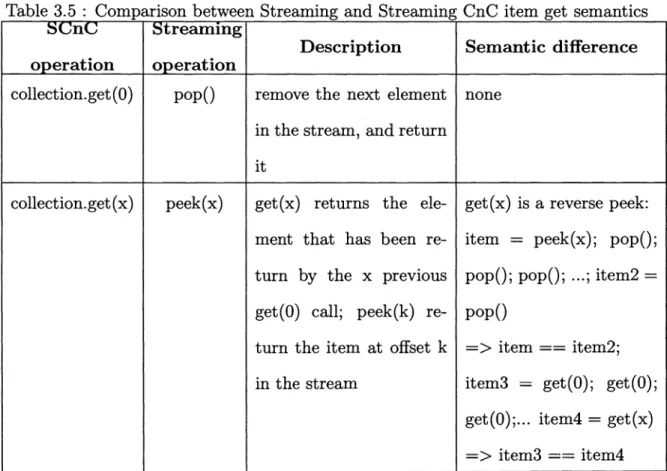
Table 3.5: Comparison between Streaming and Streaming CnC item get semantics
::Streammg
operation operation
collection.get ( 0) pop()
collection.get ( x) peek(x)
Description Semantic difference
remove the next element none in the stream, and return
it
get(x) returns the ele- get(x) is a reverse peek: ment that has been re- item = peek(x); pop(); turn by the x previous pop(); pop(); ... ; item2 = get(O) call; peek(k) re- pop()
turn the item at offset k =>item== item2; in the stream item3 = get(O); get(O);
get(O); ... item4 = get(x) => item3 == item4
Item Collection
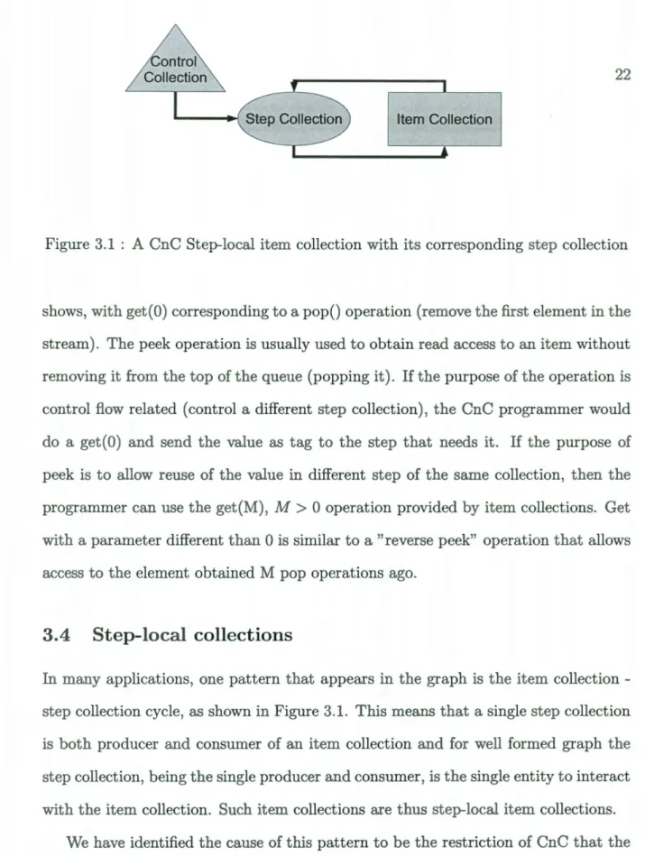
Figure 3.1 : A CnC Step-local item collection with its corresponding step collection
shows, with get(O) corresponding to a pop() operation (remove the first element in the stream). The peek operation is usually used to obtain read access to an item without removing it from the top of the queue (popping it). If the purpose of the operation is control flow related (control a different step collection), the Cn C programmer would do a get(O) and send the value as tag to the step that needs it. If the purpose of peek is to allow reuse of the value in different step of the same collection, then the programmer can use the get (M), M
>
0 operation provided by item collections. Get with a parameter different than 0 is similar to a "reverse peek" operation that allows access to the element obtained M pop operations ago.3.4
Step-local
collections
In many applications, one pattern that appears in the graph is the item collection-step collection cycle, as shown in Figure 3.1. This means that a single collection-step collection is both producer and consumer of an item collection and for well formed graph the step collection, being the single producer and consumer, is the single entity to interact with the item collection. Such item collections are thus step-local item collections.
We have identified the cause of this pattern to be the restriction of CnC that the steps are stateless (that is, there is no state information preserved between different step instance executions). If the application access pattern is streaming, these
collec-tions can be transformed back to step-local variables as state is permitted in SCnC. The definition of streaming access pattern will be covered in Chapter 4.
3.5 Dynamic Parallelism support
Changing the structure of a streaming graph is rarely required by the semantics of streaming applications [6). It might, however, be a feature that allows better performance for many applications, due to the dynamic adaptation. Streaming CnC offers a way of expressing a limited type of such changes through dynamic split-join nodes. This optimization is similar to the Streamlt fission optimization[15), only that in our case it is dynamic: the number of parallel branches of a split node can vary dynamically. In fact initially tehre does not need to be a split node.
We based the dynamic parallelism approach on the notion of places in XlO and HJ. A change to the meaning of CnC tags was performed: when a control tag is put, there one can supply an additional dimension for the tag, a place id. The code of a single filter runs in different places in parallel. When a new place id is used for the first time, the corresponding instance instance of the filter is instantiated and inserted in the graph with the same connections as the filter being prescribed , thus forming a dynamic split-join node. Each of the nodes maintain their own local data fields whose values can be used between iterations. This approach works well for situations when the programmer is aware of the additional parallelism, but does not need to write any low level synchronization or task management code. It proved useful for situations such as clustering applications or load balancing, as the Facility Location and Sieve applications described in sections 6.3.6 and 6.3.4 show.
For steps that do not use local state between step instances, we describe a com-piler transformation that would make the parallelism transparent to the code inside
the step for steps. In combination with adding automatic place distribution in the runtime, this approach has the potential of obtaining performance gains without the need for programmer-managed parallelism. As the algorithm involves knowledge of the implementation details, specifically of some phaser restrictions, it is presented later, in Section 5.2.
Chapter 4
Towards automatic conversion of Macro-dataflow
Programs to Streaming Programs
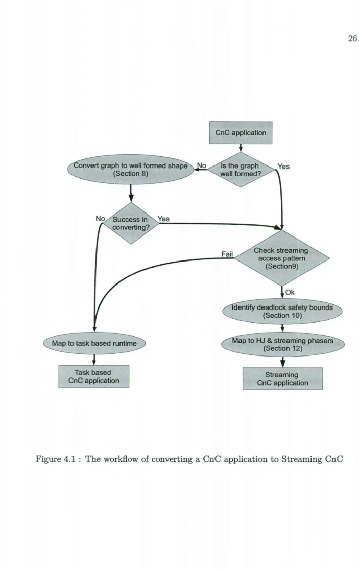
This chapter deals with automatic transformation of a CnC application that follows the classic model to one that runs on the Streaming CnC runtime, when legal to do so. The process should be similar for any transformation of a macro dataflow application to exploit streaming parallelism. In order to implement such a transformation, we considered three major steps as illustrated in Figure 4.1.
The first step is transforming the graph shape of the CnC application to a form that can be supported by theSCnC model- this transformation might not even be possible and for this step the "success in converting" will return "No". The algorithm and detailed description for this step are located in Section 4.1 .
Then, we need to check the streaming access patterns, which filters out additional non-streaming applications. We show how to do this in Section 4.2. The approach assumes the availability of functions that identify the tags (keys) for item operations performed by steps. They are under development in the Habanera CNC system, but until their implementation is complete, the contents of this chapter remains in the algorithmic realm.
As a last step, we need to convert the tags of the collections from CnC to SCnC; our approach is described in Section 4.5. This is an integral step in the mapping from the CnC API to the streaming API;our implementation is discussed later.
Convert graph to well formed shape (Section 8)
Fail Check streaming access pattern
(Section9)
4.1
Transforming a CnC graph to a well formed shape
4.1.1 Possibility and Profitability of a CnC to SCnC transformation
Some programs written for the classic CnC runtime do not respect the restrictions of SCnC mentioned in the previous chapter on interaction with the environment, on the number of producers and consumers and the number of step collections prescribed by a control collection. If they were rewritten to a SCnC conforming (well formed) shape and found to respect some runtime behaviour restrictions, as the next sections show, some of these programs could run on the streaming runtime.
In some cases, it might not be profitable to run a CnC program using the stream-ing runtime if the graph needed alteration in order to conform to the well-formed shape. Although the overhead of streaming is less than the overhead of task based runtimes and there are memory management advantages too, the parallelism of the streaming runtime is usually fixed to the number of filters in the program, whereas the parallelism in task based runtimes can potentially approach the number of dy-namic tasks in the program. We offer a solution for the limited parallelism exploited by classic streaming applications by the dynamic parallelism extension presented in later sections, but the parallelism in the classic CnC model could still be higher. At what point does the lower overhead become less profitable than simply using more parallelism is a matter of experience and practice. All our test applications benefit greatly from the streaming runtime, but it might not be always the case, depending on the parallelism available in the target hardware.
4.1.2 Algorithm for converting a CnC graph to well formed shape
The steps through which a CnC graph specification is rewritten to adhere to Stream-ing CnC well-formed shapes are the followStream-ing:
1. Rewrite the graph by adding a new step collection and control collection for interaction with the environment. The instances of this new entry collection serve as sources for the items that would have been put from the environment before transformation. To perform the transformation, redirect all starting points of item put-edges from the environment to instead start from the entry node step collection. Redirect all the put-edges from the environment to end at this node and add a control-put edge from the environment to the control collection of entry step collection. Figure 4.2 illustrates this transformation.
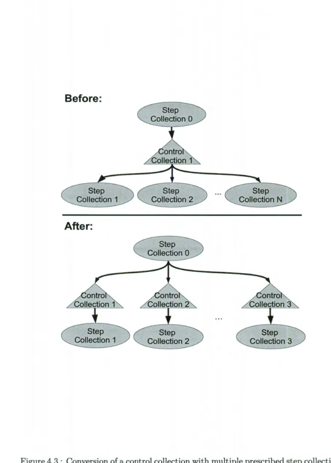
2. Rewrite the graph by adding new control collections where there are multi-prescription control collections. Do this by replacing the control collection with N prescribed step collections with N control collections. Add prescription edges from each of the new control collections to one of the step collections and edges from the producer of the initial control collection to the new control collec-tions.Figure 4.3 illustrates this transformation.
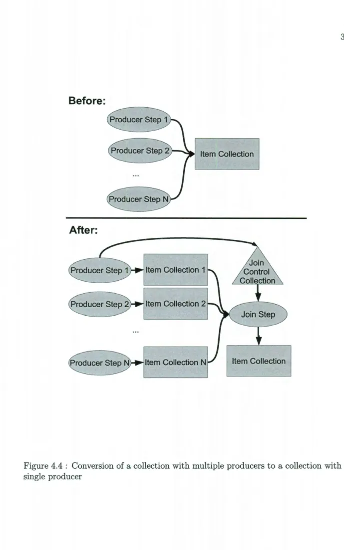
3. Reshape the graph to eliminate any multiple producer item collections. This is done by splitting the item collection and adding a step prescribed by one of the producer steps that functions as a custom join step: it gets items from all split collections and puts them into a single result collection. All the put-edges should be redirected to this step. Add a put-edge from the step to the item collection. This transformation requires also code to be inserted in the new step to perform the correct puts in the correct order, so as to obtain a custom join
Before:
Item Collection 1 Item Collection 2 Item Collection 3A
ft
e
r:
1Figure 4.2: Conversion of environment from multiple producer to single producer by adding an additional step
Before:
After:
Figure 4.3: Conversion of a control collection with multiple prescribed step collections
that assures determinism. Figure 4.4 illustrates this transformation.
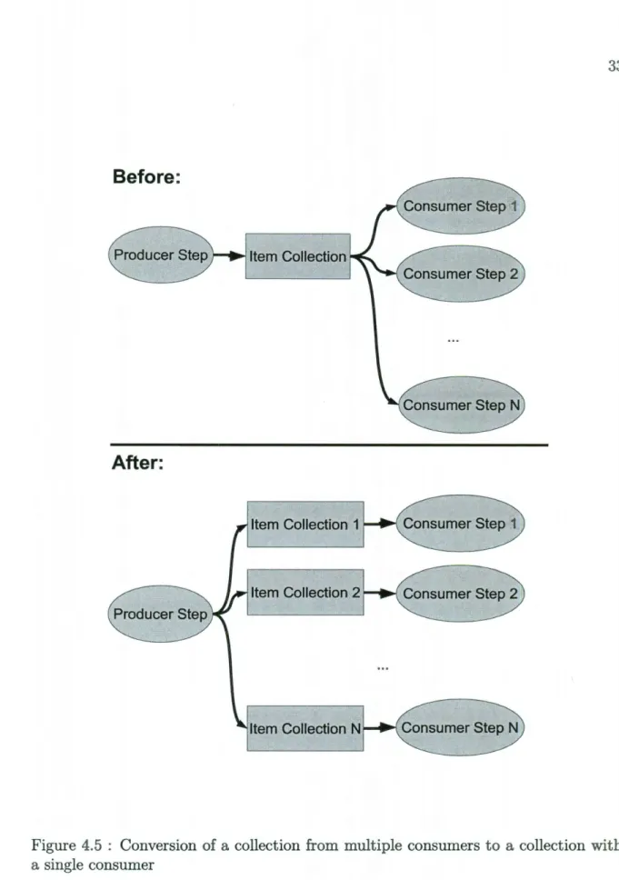
4. Duplicate any multiple consumer item collections such that they become single consumer, by duplicating the put-edges that produce items to each clone of the collection, and keeping a different single get-edge from each clone to a consumer. Figure 4.5 illustrates this transformation.
The pseudocode for the transformation algorithm follows.
1 If (environment is multiple-producer) {
2 insert new step EntryStep and prescription collection EntryTags
3 add prescription edge EntryTags -> EntryStep
4 redirect edges starting from environment to start from EntryStep
5 add producer edge from the environment to EntryTags
6 }
7 / / correct the control collections first
s insert all control collections in the worklist
9 while (worklist not empty) {
10 pop control collection crt from the worklist
n if (crt is multiple prescription) {
12 add n control collections
13 add a edges from one collection to one of the step collections
14 add edge from producer of crt to each new collection
15 remove crt and its edges
16 } 17 }
1s Insert all item collections in the worklist
19 while (worklist not empty) {
20 pop item collection crt from worklist
21 If (crt has multiple producers) {
Before
:
Item Collection
After
:
Item Collection 1
Item Collection 2
Item Collection N Item Collection
Figure 4.4 : Conversion of a collection with multiple producers to a collection with a single producer
Before
:
Producer Step Item Collection
Consumer Step N
After
:
Item Collection 1 Consumer Step 1
Item Collection 2 Consumer Step 2
Producer Step
Item Collection N
Figure 4.5 : Conversion of a collection from multiple consumers to a collection with a single consumer
23 r e d ire c t each edge to one of the item c o ll e c t i o n s
24 add collections
ci
to worklist25 add tag collection TJ and join step collection SJ
26 add prescription edge T J- > SJ
27 add item consumer edges from each Ci to SJCi- > SJ
28 add item producer edge from SJ to crt SJ- >crt
29 }
30 If (crt has multiple consumers) {
31
I I
crt has a single producer now32 remove crt
33 add an item collection Ci for each consumer crt had
34 add each Ci to the worklist
35 add item consumer edges from each Ci to a consumer
36 add item producer edges from the producer step or crt p to each Ci
37 }
38 }
4.1.3 Algorithm analysis
In this section, we analyze the complexity of the transformed graph relative to the input graph. Of course, if the input graph is already well formed, then no further transformation is needed.
The addition of nodes and edges in the course of the transformations mentioned could lead to two sources of overhead: additional memory consumption because of the new item collections added and additional synchronization from the additional edges added. For example, a conversion from a multiple producer item collection to single producer adds N item collections, one for each separate producer, and a new step collection with associated control collections. The space requirements grows N
+
1times (N item collections+ 1 control collection), though this space requirement may be reduced in a later transformation when item collections are replaced with bounded buffers.
Synchronization requirements cannot be easily compared because the CnC syn-chronization is different from SCnC one. Let us assume that synsyn-chronization overhead is proportional to the number of edges (in SCnC, a pair of edges results in the use of a phaser; in CnC depending on the runtime, synchronization mechanisms vary, but the synchronization overhead remains proportional to the number of collections ) .
For the same example of multiple to single producer transformation for item col-lections, the number of edges in the figure increases from 4 to 9. In the general case of N producers, the number of edges increases from N to 2*N+2+1 edges, which leads to a doubling in the number of buffers.
Another limitation, caused by our use of explicit join nodes as opposed to implicit joins, is the inability of performing optimizations based on the relative flow rates as these are hidden inside user code. We considered the option of having the puts and joins of a step be part of its signature, but we chose not to do so - we would lose the flexibility of variable input output rates and thus not been able to support all well formed SCnC graphs.
4.2 Identifying streaming patterns in a well formed CnC
graph
The Concurrent Collections model allows for the distinction between the domain ex-pert (who writes the CnC graph and maybe the step code) and the tuning exex-pert (who optimizes the application for best performance, by setting CnC scheduling
pa-rameters, adding scheduling restrictions and optimizing the step code).
As the streaming runtime is more restrictive than the task based one, additional checks have to be made before using it. First, the expert has to determine if the application can be rewritten to a streaming shape. To do this, we proposed in Section 4.1 an algorithm that can check for the structural graph requirements of the streaming parallel model. The current section deals with the required checks for the streaming access patterns on a well-formed graph, as in the output of the algorithm presented in Section 4.1.2. In this section, we take the well-formed shape of the application graph as a given and use the theorems 3.1 and 3.2 to support our analysis.
The proposed algorithm has two phases: graph analysis (computing auxiliary information) and streaming checks. The second phase can throw errors indicating that the application cannot be transformed to streaming form using our algorithm.
Any step that requires the computation of a function that cannot be solved (func-tion does not exist) will fail and lead to early termina(func-tion of the algorithm with an output of FALSE (application cannot be converted to streaming form using simple rewrite rules).
The graph analysis phase consists of the following steps:
1. Require the tags of the EntryStep collection (the Env-
>
EntryTags edge) to be consecutive integers starting from 0 and the tags of all other control collections to be integers. It is possible to relax this restriction by allowing tags that contain an integer component.2. Annotate each item-put edge (between a step T and an item collection 0) with at least one put-function with domain the possible step prescription tags for step T and codomain the tags of the items that are put. There should be a
put-function for each tag that can possibly correspond to an item put by the step. If a step instance puts at least k items, there have to be at least k put-functions, to model the relationship between the tag of the step and the tag of the items produced.
3. Annotate each tag-put relationship with (at least one) function f1agPut with the same eaning as in the previous step.
4. Annotate each item-get relationship with (at least one) function fftemGet similar to the previous functions, but for item get operations.
5. Label each prescription edge with the identity function ftagGet(x) = x.
6. Do a traversal of the CnC control graph (which, for a well formed CnC graph, is an arborescence according to Theorem 3.2), labelling each step collection and attached item collection with the result of the composition of the func-tions through which the path from the root of the tree passes to reach that particular step. We call this label function a producer function for that step. f;: = fnUn-1Un-2( ...
fi))))
where the path from root EntryStep to Stepn passes though Steps n-1, n-2, .... , 1 and Step1 is EntryStep. The identify functions can safely be folded away in this chain. The traversal is easily done in a preorder traversal of the CnC control graph, thus incurring only a linear complexity cost. At each step collection node in the graph, label it with the same producer func-tions of its parent tag collection. At each tag collection node, label it with the composition of the producer functions of the parent and its incoming tag-put function. The producer functions for each step collection there will result in an associated set of producer functions, as control collections can have multiple incoming tag-put functions, depending on the producing step collection code.f ta Put (t)
=
t Bank1_0id f (t)=
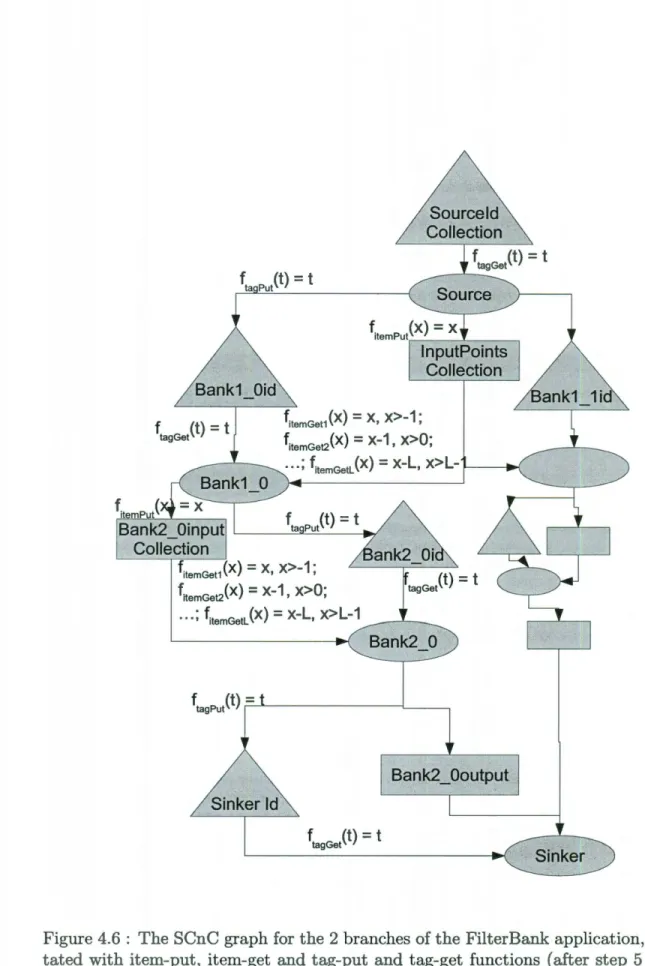
t tag Get fitemGet1(X) =X, X>-1; fitemGet2(x) = X-1' x>O; ·· .; fitemGetL(x) =X-L, x>l-~----~~ Ban k2 _ Oinput '---'-~~-__..,. Collection fitemGet1 (X) = X, X>-1; fitemGet2(x) = x-1' x>O; ... ; fitemGetL (x) = X-L, x>l-1 f tagPut (t)-r----"~---1___----, f tag Get (t)=
tFigure 4.6: The SCnC graph for the 2 branches of the Filter Bank application, anno-tated with item-put, item-get and tag-put and tag-get functions (after step 5 of the algorithm)
f ta Put (t)
=
tfc
1(x) =X, x>-1; f (x)=
x-1 x>O· c2 ' '... ;
fc
L (x)=
x-L, x>L-1 f (t)=
t inker I f (t)=
t tag Get Source f (x) = x itemPut (x)=
X lnputPoints Collection Bank2 0 f (x) = x p 1 - - - , f (x)=
x c Bank2_ Ooutputfc(x)
=
X..__ _ _ - - - i f tag Get (t) = tFigure 4.7: The SCnC graph for the 2 branches of the Filter Bank application,
anno-tated with producer and consumer functions for item collections, after applying the algorithm
7. For each item collection, label it with a consumer-function fc by composing the get function fltemGet of the item collection outward edge with the producer function of the consumer step.
8. For each item collection, label it with (at least one) producer-function by com-posing the get function fltemGet of the item collection producer edge with the producer function of the producer step. Both steps are made possible because the CnC graph we are working on has previously been reshaped to a well formed shape.
9. For each step compute the minimum consumer function, defined as the minimum of the values of all the consumer functions for each pair of (step, consumed item collection),
f
em in (y) = minx Ucx(y)),
\ly ·All these functions will be used in the testing phase to ensure that the application access patterns are streaming. Note that, according to Theorem 3.2 if there are functions for steps 2 to 5, then the composition of functions required for step 6 exists (the set of producer functions that are attached to each node will have at least one element). The only way this algorithm can fail is if steps 2-4 in the testing phase fail to find a function.
The purpose of the test phase is to test the fact that the graph functions respect the streaming access restrictions to items. It consists of the following steps:
1. Using the consumer-functions and producer-functions of the item collections, we can test if the application is streaming or not. There may be multiple producer functions and multiple consumer functions for a single item collection and they will all have to be taken into consideration. Producer functions have to output consecutive increasing values for consecutive increasing inputs.
2. Test that the producer functions inverse and consumer functions for all item collections respect the following three conditions:
a. "producer precedence" constraint, expressed through the following equation: fp-1(y)
<
J;
1(y), 'r:/y>
0. If there is no inverse for either producer or consumerfunctions for any item collection or if the previous relationship does not hold, the application is not a SCnC streaming application.
b. "bounded buffer" constraint: there exists a constant N such that for any pair of consumer functions
fc
1 andfc
2 of a step collection, the difference between the value of the consumer functions is smaller than N. The constraint is expressed though the equation where x the time iterations/sequence numbers put from the environment as tags in step 1 of the analysis phase:l(fc1 - !c2)(x)l
<
N, 'r:/x and 'r:/
fc
1 and 'r:/fc
2 consumer-functions of a single step collection. This is a restriction of the more general streaming requirement that once item i with tag t has been accessed, one can only access items with tags higher thant-N.
c. "sliding window" constraint: For a single step collection, but different con-secutive step instances tagged y and y+1, the minimum value of the tag that can be consumed by that step tagged y+1 is not lower than the minimum value that can be consumed by step instance tagged y.
f
cmin (y)< f
cmin (y + 1) The bounded buffer and sliding window constraints guarantee that we will never need a buffer size larger than N for an item collection.d. "bounded lifetime" constraint: For any item tagged t, produced in iteration
t1 and consumed in iteration t2 , there is N2 constant such that t2 - t1
<
N2 Bounded buffer, sliding window and bounded lifetime assure that we will notneed a buffer size larger than N1 or N2 to satisfy get calls on an item collection. e. "unique timestep" constraint: Each step instance performs no more than a single put in each of its output control collections. This constrain assures us that, for a given step collection there will never be more than one step instance with the same iteration number (started by a single ancestor).
If the functions of all item collections respect the previous constraints, then the algo-rithm outputs TRUE. Otherwise it outputs FALSE.
Theorem 4.1
For an application with a well formed CnC graph, if the producer and consumer func-tions exist and respect the bounded buffer, producer precedence and sliding window rules and the CnC application terminates (with no suspended steps/deadlocks), then the corresponding SCnC application, if it terminates, terminates with the exact same state than the CnC application. The state of the CnC application consists of the items it has produced in each of the item collections.
Proof 4.1 In order to have item collections with the same items, the same steps should run and steps must have the same inputs and must produce the same outputs.
The first condition for this to happen is for the desired inputs to be available; the proof for this is as follows. The "bounded buffer" and "sliding window" constraints prohibit the access to items that are not in the streaming buffer of size N: bounded buffer means that a single step execution will need to access more items than the buffer has space for (accesses max N elements) and the sliding window rule shows that no step will need access to items that have already been removed (they can only access items that are "newer" than the oldest item consumed by the previous step). If neither the execution of a single step nor the sequence of two step executions lead
to accessing an item that will not correspond to the CnC one, then, by induction, any execution will not lead to this situation.
The second condition is that the steps executed are the same in both SCnC and CnCand have identical inputs and outputs. They are, as no code changes are needed for well formed graphs, except the conversion of tags, but that transformation affects only the the tag keys, not the values accessed by them. Steps are executed on the same input identified as a subset from the codomain of the item put functions, by the step code, whose control flow is governed by the control tags which are explicitly and identically sent through the corresponding stream. As proved in the previous paragraph, the selected items are available. As the control flow is identical, then the items produced are identical. 0
4.3 Deadlock
The question remains: can the SCnC version "hang" when the CnC application does not? We show that the SCnC application hangs only because of insufficient buffer-size problems that are common to all streaming programs.
First, let's look at when a CnC application can hang. A CnC application can hang if a step hangs. A step hangs if an item that is the target of a get is not produced in a finite amount of time. This can happen if the producer step hangs(reducing the problem to a previous step) or the producer step is not run because it is never prescribed. If we presume the CnC application does not hang, then none of these problems appear for the SCnC implementation.
A SCnC application can hang for any of the causes that a CnC application can hang, plus the following: