University of Huddersfield Repository
Zhang, Wei Emma, Sheng, Quan Z., Taylor, Kerry, Qin, Yongrui and Yao, Lina
Learningbased SPARQL Query Performance Prediction
Original Citation
Zhang, Wei Emma, Sheng, Quan Z., Taylor, Kerry, Qin, Yongrui and Yao, Lina (2016) Learning
based SPARQL Query Performance Prediction. In: The 17th International conference on Web
Information Systems Engineering (WISE), November 7 10, 2016, Shanghai, China.
This version is available at http://eprints.hud.ac.uk/29767/
The University Repository is a digital collection of the research output of the
University, available on Open Access. Copyright and Moral Rights for the items
on this site are retained by the individual author and/or other copyright owners.
Users may access full items free of charge; copies of full text items generally
can be reproduced, displayed or performed and given to third parties in any
format or medium for personal research or study, educational or notforprofit
purposes without prior permission or charge, provided:
•
The authors, title and full bibliographic details is credited in any copy;
•
A hyperlink and/or URL is included for the original metadata page; and
•
The content is not changed in any way.
For more information, including our policy and submission procedure, please
contact the Repository Team at: [email protected].
http://eprints.hud.ac.uk/
Prediction
Wei Emma Zhang1
, Quan Z. Sheng1
, Kerry Taylor2
, Yongrui Qin3
, and Lina Yao4
1
School of Computer Science, The University of Adelaide, Australia
2
Research School of Computer Science, Australian National University, Australia
3
School of Computing and Engineering, University of Huddersfield, UK
4
School of Computer Science and Engineering, UNSW Australia, Australia
Abstract. According to the predictive results of query performance, queries can be rewritten to reduce time cost or rescheduled to the time when the resource is not in contention. As more large RDF datasets appear on the Web recently, predicting performance of SPARQL query processing is one major challenge in managing a large RDF dataset ef-ficiently. In this paper, we focus on representing SPARQL queries with feature vectors and using these feature vectors to train predictive models that are used to predict the performance of SPARQL queries. The eval-uations performed on real world SPARQL queries demonstrate that the proposed approach can effectively predict SPARQL query performance and outperforms state-of-the-art approaches.
Keywords: SPARQL, Feature Modeling, Prediction
1
Introduction
The Semantic Web, with its underlying data model RDF and its query lan-guage SPARQL, has received increasing attention from researchers and data consumers in both academia and industry. RDF essentially represents data as a set of three-attribute tuples, i.e., triples. The attributes aresubject, predicate
andobject, where predicate is the relationship betweensubject andobject. Over the recent years, RDF has been increasingly used as a general data model for conceptual description and information modeling. Since the number of publicly available RDF datasets and their volume grow dramatically, it becomes essential to provide efficient querying of large scale RDF datasets. This is an important is-sue in the sense that whether to obtain knowledge efficiently affects the adoption of RDF data as well as the underlying Semantic Web technologies.
Substantial works focus on the prediction of query performance (e.g., execu-tion time) [16, 9, 1]. Predicexecu-tion of query execuexecu-tion performance can benefit many system management decisions, including workload management, query schedul-ing, system sizing and capacity planning. Studies show that cost model based query optimizers are insufficient for query performance prediction [2, 6]. There-fore, approaches that exploit the machine learning techniques to build predictive
models have been proposed [2, 6]. These approaches treat the database system as a black box and focus on learning a query performance predictive model, which are evaluated as feasible and effective [2]. These works extract the fea-tures of queries by exploring the query plan which can provide estimations such as execution time, row count and these two estimations for each operator.
However very few efforts have been made to predict the performance of SPARQL queries. SPARQL query engines can be grouped into two categories: RDBMS-based triple stores and RDF native triple stores. RDBMS-based triple stores rely on optimization techniques provided by relational databases. How-ever, due to the absence of schematic structure in RDF, cost-based approaches show problematic query estimation and cannot effectively predict the query per-formance [15]. RDF native query engines typically use heuristics and statistics about the data for selecting efficient query execution plans [14]. Heuristics and statistics based optimization techniques generally work without any knowledge of the underlying data, but in many cases, statistics are often missing [15]. Has-san [8] proposes the first work on predicting SPARQL query execution time by utilizing machine learning techniques. The key contribution of the work is to model a SPARQL query to a feature vector, which can be used in machine learning algorithms. However, in practice, we observe that modeling approach is very time consuming. To address this issue, we leverage both syntactical and structural information of the graph-based SPARQL queries and propose to use the hybrid features to represent a SPARQL query. Specifically, we transform the algebra and BGPs of a SPARQL query into two feature vectors respectively and perform a feature selection process based on heuristic to build hybrid features from these two feature vectors. Our approach reduces the computation time of feature modeling in orders of magnitude. Once the features are built, we use machine learning algorithms to train the prediction model. The input of the al-gorithm is the feature matrix of the training queries (we concatenate the feature vectors of individual queries into a matrix) and the query performance of these queries (here we only consider the elapsed time used to perform a query and get the result). The output is the trained prediction model. When a new query q is issued, we obtain its feature vector using our feature modeling approach. Then we use the trained prediction model to predict the performance of q. K-Nearest-Neighbor (KNN) regression and Support Vector Regression (SVR) are both considered as the predictive model. We develop a two-step prediction pro-cess to improve the prediction result compared to one-step prediction.Moreover, we evaluate our approach on both cold (i.e., fresh queries) and warm (i.e., re-peated queries) stages of the system. In cold stage, elapsed time consists of both compile and execution time while in warm stage, elapsed time equals to the exe-cution time. The reason we can ignore the compile time is because our work only considers static querying data. Thus a repeated query has the same execution plan each time it is issued and the system only compiles once. The consideration of cold stage is useful as the knowing of execution performance for unseen queries is more important for system management than to previously seen queries.
Our approach can be applied in the situation that no estimation of query ex-ecution performance are provided, or such estimations are implicit or inaccurate. In practice, this applies to most triple stores that are publicly accessible. More-over, no domain expertise is required. All the methods are easy to reproduce as we choose the most commonly used algorithms in the the machine learning field. In a nutshell, the main contributions of this work are summarized as follows:
– We adopt machine learning techniques to predict the SPARQL query perfor-mance before their execution. We transform the SPARQL queries to feature vectors that is required by the machine learning algorithms. Hybrid feature modeling is proposed based on the features that can be obtained without the information of the underlying systems.
– We consider both warm and cold stage prediction, and the latter one has not been discussed in the state-of-the-art works, but is important to the examination of execution performance of a query.
– We perform extensive experiments on real-world queries obtained from widely accessed SPARQL endpoints. The triple store we used is one of the most widely used systems in the Semantic Web community. Thus our work can benefit a large population of users. Moreover, our approach is system inde-pendent that can be applied to other triple stores.
The remainder of this paper is structured as follows. Existing research efforts on the related topics are discussed in Section 2. In Section 3, the background knowledge is briefly introduced. Section 4 describes our prediction approaches in detail. Section 5 reports the experimental results. Finally, we discuss some issues we observed and conclude the paper in Section 6.
2
Related Work
There are very limited previous works that pertain to predicting query perfor-mance via machine learning algorithms in the context of SPARQL queries. We introduce here the works of predicting SQL queries performances that we draw ideas from and discuss the work in [8].
Akdere et al. [2] propose to predict the execution time using Support Vec-tor Machine (SVM). They build predicVec-tors by leveraging query plans provided by the PostgreSQL optimizer. The authors also choose operator-level predictors and then combine the two with heuristic techniques. The work studies the ef-fectiveness of machine learning techniques for predicting query latency of both static and dynamic workload scenarios. Ganapathi et al. [6] consider the prob-lem of predicting multiple performance metrics at the same time. The authors also choose query plan to build the feature matrix. Kernel Canonical Correla-tion Analysis (KCCA) is leveraged to build the predictive model as it is able to correlate two high-dimension datasets. As addressed by the authors, it is hard to find a reverse mapping from feature space back to the input space and they consider the performance metric of KNN to estimate the performance of target query. Hassan [8] proposes the first work on predicting SPARQL query execution
time by utilizing machine learning techniques. In the work, multiple regression using SVR is adopted. The evaluation is performed using benchmark queries on an open source triple store Jena TDB5
. The feature models are extracted based onGraph Edit Distances (GED) between each of training queries. However, in practice, we observe that the calculation of GED is very time consuming, which is not a desirable method when the training dataset is large. Our work draws idea from this work and improves it by largely reducing the computation time.
3
Preliminaries
3.1 SPARQL Query
A SPARQL query can be represented as a graph structure, the SPARQL graph [7]. Given the notation B, I, L, V for the (infinite) sets of blank nodes, IRIs, literals, and variables respectively, a SPARQL graph pattern expression is defined recursively (bottom-up) as follows [11]:
(i) A valid triple pattern T ∈ (IV B)×(IV)×(IV LB) is a basic graph pat-tern (BGP), where a triple patpat-tern is the triple that any of its attributes is replaced by a variable.
(ii) ForBGPi andBGPj, the conjunction (BGPi andBGPj) is a BGP. A BGP
is a graph pattern.
(iii) IfPi andPj are graph patterns, then (PiANDPj), (Pi UNIONPj) and (Pi
OPTIONALPj) are graph patterns.
(iv) If Pi is a graph pattern andRi is a SPARQL build-in condition, then the
expression (Pi FILTERRi) is a graph pattern.
3.2 Multiple Regression
Multiple Regression focuses on finding the relationship between a dependent variable and multiple independent variables (i.e., predictors). It estimates the expectation of the dependent variable given the predictors. Given a training set (xi, yi), i= 1, ...n, wherexi ∈Rmis am-dimensional feature vector (i.e., m
predictors), the objective of multiple regression is to discover a functionyi=f(xi)
that best predicts the value ofyi associated with eachxi [12].
Support Vector Regression is to find the best regression function by selecting the particular hyperplane that maximizes the margin, i.e., the distance between the hyperplane and the nearest point [13] . The error is defined to be zero when the difference between actual and predicted values are within a certain amount ξ. The problem is formulated as an optimization problem:
minwTw, s.t. yi(wTxi+b)≥1−ξ, ξ≥0 (1)
5
✁ ✂ ✄☎✆ ☎ ✆✝✟✠ ✡✂ ☎✡☛ • ☞✡✌✍ ✎✡ • ✏✑ ✒ ✂ ✄✌✒☎✆ ✓ ✍✂ ✔✄✒ ☎ ✍✆ • ✕✡✔✍✖✡☎✆✖✄✗☎ ✎✘✠ ✡ ✂ ☎✡☛ &ĞĂƚƵƌĞDŽĚĞůůŝŶŐ WƌĞĚŝĐƚŝǀĞDŽĚĞůdƌĂŝŶŝŶŐ ✌✗✡✄✆✘✠ ✡ ✂ ☎ ✡☛ ✙✡✄✒✠ ✂✡✔✄✒ ✂☎✑ • ✙✡✄✒✠✂✡✚✡✗✡ ✌✒ ☎ ✍✆ • ✕✡ ☛✌ ✄✗☎✆✝ ✟✠ ✡ ✂✛✕✡✘✠✡☛ ✒ ĂƚĂWƌĞͲƉƌŽĐĞƐƐŝŶŐ ✜ ✂✡✎☎ ✌ ✒✡ ✎✂✡ ☛ ✠✗✒☛ ✙✡✄✒✠✂✡✖✡✌✒ ✍✂ ✜✂✡✎☎✌✒☎ ✍✆ ✢ ✍✎✡✗ ✣✗✄☛☛☎✓ ☎ ✌ ✄✒☎ ✍✆ ✞✤✥✦✧✤ ★ ✩✪✤✫ ✬✭ ✧✬✮ ✞ ✯✰✮ ✥✦✧✤★ ✩✪✤✫ ✬✭ ✧✬✮ ✞ ✁ ✂ ✄☎✆☎ ✆ ✝ ✟✠ ✡ ✂ ☎✡ ☛ ✱✄✲✡✗☎✆ ✝
Fig. 1.Steps for Query Performance Prediction
where parameter b
kwk determines the offset of the hyperplane from the origin
along the normal vectorw. If we extend the dot product ofxi·xj to a different space of larger dimensions through a functional mappingΘ(xi), then SVR can
be used in non-linear regression. Θ(xi)·Θ(xj) is called kernel function. An
advantage of SVR is its insensitivity to outliers [17].
K-Nearest Neighbours is a non-parametric classification and regression method [3]. The KNN regression predicts based on K nearest training data. It is often successful in the cases where the decision boundary is irregular, which applies to SPARQL queries [8]. By training the KNN model, the predicted query time can be calculated by the average time of its K nearest neighbours.
tQ = 1 k k X i=1 (ti) (2)
whereti is the elapsed time of theith nearest query.
4
SPARQL Query Performance Prediction
Our prediction process consists of four main phases, namelyData Pre-Processing,
Feature Modeling,Predictive Model Training andPrediction(one-step and two-step) (Figure 1). Both training and new requested queries are cleaned in the
Data Pre-Processing phase, valid queries are extracted during this phase. In theFeature Modeling phase, queries are represented as a set of features. In the
Predictive Model Trainingphase, predictive models are derived from the train-ing queries with observed query performance metrics. In the Prediction phase, trained predictive models are used to predict the performance of a new issued
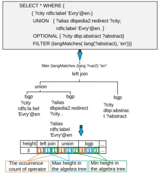
?city rdfs:la bel 'Evry'@en ?alias dbpedia2:redirect ?city . ?alias rdfs:label 'Evry'@en bgp ?city dbp:abstrac t ?abstract bgp bgp union left join filter (langMatches (lang ?var2) "en"
left join union bgp
1 1 1 1 2 2 3 3 3 The occurrence
count of operator
Max height in the algebra tree
Min height in the algebra tree
... ... height
3
SELECT * WHERE {
{ ?city rdfs:label 'Evry'@en.}
UNION { ?alias dbpedia2:redirect ?city; rdfs:label 'Evry'@en. } OPTIONAL { ?city dbp:abstract ?abstract} FILTER (langMatches( lang(?abstract), 'en'))}
Fig. 2.Algebra Feature Modelling on Example Query
query. Compare to one-step prediction, the two-step prediction has labeling be-fore predictive model training and classification step bebe-fore prediction. We focus on discussion of feature modeling in Section 4.1 and describe the predictive mod-els training and two-step prediction in Section 4.2. We ignore the description of data pre-processing due to the space constraint.
4.1 Feature Modeling
In order to utilize machine learning algorithms for SPARQL query performance prediction, we transform the SPARQL query into vector representation where each value in a vector is regarded as a feature instance of a query. The perfor-mance of prediction highly depends on how much information the features can represent the data. In this study, we use only static, compile time features that are extracted prior to execution. The algebra and BGP features are obtained by parsing the query text (Section 4.1.1 and 4.1.2). The hybrid features are gener-ated by applying a selection algorithm on the algebra and BGP features (Section 4.1.3). We concatenate the feature vectors of a set of training queries and form a feature matrix as the input of learning algorithms.
4.1.1 Algebra Feature The algebra of a SPARQL query can be presented
as a tree where the leaves are BGPs and nodes are operators presented hierar-chically. The parent of each node is the parent operator of current operator. We
✁
✂✄ ☎ ✂✄ ✁ ✂☎ ✆✂✄✝✁✝☎✟ ✆✂✄✝✁✝✂☎✟
Fig. 3.Example Triple Patterns
traverse the tree to construct a set of tuples {(opti, ci, maxhi, minhi)}, where opti is the operator name,ciis the occurrence count ofopti in the algebra tree, maxhi and andminhi areopti’s maximum height and minimum height in the
algebra tree, respectively. We then concatenate all the tuples sequentially to form a vector. We further insert the tree’s height at the beginning of the vector. Figure 2 illustrates an example of algebra feature modelling.
4.1.2 BGP Feature Algebra features takes occurrences and some
hierarchi-cal information of operators into consideration, but fails to represent BGPs, the most widely used subset of SPARQL queries [4]. To represent BGPs, we propose to build BGP features. We examine that BGPs consist of sets of triple patterns (Section 3) thus can also be represented as tree structure. But we choose not to use similar transform approach (i.e., record occurrences and maximum/min-imum heights) as in algebra feature modelling. Instead, we propose a new way to transform BPGs to vector representation for comparison.
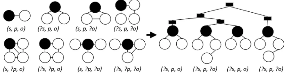
Specifically, we leverage the edit distance between graphs to build BGP fea-tures because it can capture complete information of a BGP graph. Figure 3 illustrates the graph representation of two triple patterns(?s, p, o) and(?s, p, ?o) where the subject(s) and object(o) are nodes and predicate(p) are edges. The question mark indicates that the corresponding component is a variable. However, it is hard to tell the differences between the two graphs, as they are structurally identical. To address this problem, we propose to map the 8 types of triple patterns to 8 structurally different graphs, as shown in Figure 4(left). The black circles are inner conjunction nodes. To exemplify, we model the triple patterns of BGPs in the example query in Figure 2, to a graph, which is depicted in Figure 4(right). The black rectangles are outer conjunction nodes.
✁✂✄✆✄✝✞ ✟ ✁✝ ✂✄✆✄✞✟ ✁✂ ✄✆✄✞✟ ✁✂✄✝ ✆✄✝ ✞ ✟ ✁✂✄✝ ✆ ✄✞ ✟ ✁✝ ✂✄✆✄✝✞✟ ✁✝✂✄✝✆ ✄✝✞ ✟ ✁✝✂ ✄✝✆ ✄✞ ✟ ✁ ✝ ✂ ✄✆ ✄✞✟ ✁✝✂✄✆✄✝ ✞✟ ✁✝✂✄✆✄✞✟ ✁ ✝ ✂ ✄✆ ✄✝✞ ✟
Fig. 4.Mapping Triple Patterns to Graphs. Left: 8 types of triple patterns are mapped to 8 structurally different graphs. Right: mapping example query in Figure 2 to a graph.
We then calculate the Graph Edit Distance (GED)6
between the graph of a queryqand graphs of some representative queries and regard each distance as an instance of a feature. Thus we obtain an-dimensional feature vector forq, where nis the number of representative queries. We choose to use the 18 valid out of 22 templates from DBPSB benchmark [10] to generate representative queries. We build the graph for each of the 18 queries and record the GED between q and these graphs. Thus we obtain a 18-dimension feature vector forq.
4.1.3 Hybrid Feature We build hybrid feature vector forqby selecting the
most predictive features based on the algebra and BGP features. Most feature selection approaches rank the candidate features (often based on their corre-lations) and use this ranking to guide a heuristic search to identify the most predictive features. In this paper, we use a similar forward feature selection al-gorithm, but we choose the contribution to overall prediction performance as the heuristic. The algorithm starts with building predictive model (we use KNN as the predictive model here) using a small number of features and iteratively build more complex and accurate model by using more features. In each iter-ation, a new feature is tested and added to the feature set. If it improves the overall prediction performance, the feature is selected. Otherwise, it is removed from the feature set. Finally, we simply consider the completion of traversing all features as the stopping condition. The output of the algorithm is the list of selected features that form the feature vector for each query.
4.2 Prediction
We propose two prediction processes, namely one-step prediction and two-step prediction. In the one-step prediction, feature vector of a new query is input into the trained predictive model obtained in the predictive model training phase. The output is the predicted value of the query performance metrics. The two-step prediction differs with one-two-step prediction by adding classification two-step. We present the predictive models used in this work in Section 4.2.1 and describe how we do two-step prediction in Section 4.2.2.
4.2.1 Predictive Models We choose two regression approaches SVR and
KNN regression in this work (Section 3.2). The models are trained with the actual query performance of training queries and then be used to estimate the performance of a new issued query. Both models require the features vector-represented. We compare several variations of these two models in this work. The description is as follows.
6
Graph edit distance is the minimum amount of edit operations (i.e., deletion, inser-tion and substituinser-tions of nodes and edges) needed to transform one graph to the other.
SVR Four commonly used kernels are considered in our model: namelyLinear,
Polynomial, Radial Basis and Sigmoid, with different kernel parameters γ and r:
– Linear:K(xi,xj) =xTi xj
– Polynomial:K(xi,xj) = (xTi xj)r
– Radial Basis:K(xi,xj) =exp(−γ||xi−xj||2
), γ >0
– Sigmoid:K(xi,xj) =tanh(γxTi xj) +r
KNN We apply three variations of KNN regression by considering different weighting methods to the neighbors.
– Average. We assign equal weights to each of the K nearest neighbors and get the average of their elapsed time as the predicted time:
tQ= 1 k k X i=1 (ti) (3)
whereti is the elapsed time of theith nearest query.
– Power. The weights in Power is the power value of weighting scale α. The predicted query time is calculated as follows:
tQ = 1 k k X i=1 (αi∗ti) (4)
whereαi is the weight of theith nearest query.
– Exponential. We apply an exponential decay function with decay scaleβ to assign weights to neighbors with different distance.
tQ= 1 k k X i=1 (e−di∗β∗ ti) (5)
wheredi is the distance between target query and itsith nearest neighbor.
All the scaling parameters are chosen through 5-fold cross-validation.
4.2.2 Two-Step Prediction We observe that the one-step prediction, where
all the training data are fed into a single predictive model, gives undesirable performance. A possible reason is the fact that our training dataset has queries with various different elapsed time ranges. Fitting a curve for such irregular data points is often inaccurate. Then we propose a two-step prediction process, where we split queries according to their elapsed time and train different predictive models. Specifically, we firstly put the training queries in four bins, namelyshort,
medium short, medium, and long. The time ranges in these four bins are<0.1 seconds, 0.1 to 10 seconds, 10 to 3,600 seconds, and>3,600 seconds respectively. We correspondingly label all the training queries with these four labels. Then we
train four predictive models and one for each bin (or class). When a new query qarrives, we perform classification forqand obtain its label (or class). Here we use Support Vector Machine (SVM) as classification algorithm as it is the mostly used classification algorithm. Then we use the trained predictive model for the class that qis labelled to predictq’s performance.
5
Experiments
5.1 Setup
Data We used real world queries gathered from USEWOD challenge7
, which provides query logs from DBPedia’s SPARQL endpoint8
(DBpedia3.9). We ran-domly chose 10,000 valid queries in our prediction evaluation. Then these queries were executed 11 times as suggested in [7], including the first time as cold stage, and the remaining 10 times as the warm stage. Finally, we split the collection to training and test sets according to the 4:1 tradition. We set up a local mirror of DBpedia3.9 English dataset to execute the queries.
System The backing system of our local triple store is Virtuoso 7.2, installed on 64-bit Ubuntu 14.04 Linux operation system with 32GB RAM and 16 CPU. All the machine learning algorithms are performed on a PC with 64-bit Windows 7, 8GB RAM and 2.40GHZ Intel i7-3630QM CPU.
Implementation We used SVR for kernel and linear regression available from LIBSVM [5]. KNN and weighted KNN regression was designed and implemented using Matlab. The algebra tree used for extracting algebra features was parsed using Apache Jena-2.11.2 library, Java API. Graph edit distance was calculated using the Graph Matching Toolkit9
.
Evaluation Metric We followed the suggestion in [2] and used themean relative erroras our prediction metric:
relativeerror= 1 N N X i=1 |actuali−estimatei| actualmean (6) The difference with the calculation in [2] is that we divideactualmeaninstead of actuali because we observe there are zero values foractuali.
5.2 Models Comparison
We compared the Linear SVR and SVR with three kernels, namely Polynomial, Radial Basis and Sigmoid with KNN when K=1. The feature model used in
7 http://usewod.org/ 8 http://dbpedia.org/sparql/ 9 http://www.fhnw.ch/wirtschaft/iwi/gmt
Table 1.Relative Error of Elapsed Time Prediction (One-step) Elapsed time (Cold) Elapsed time (Warm)
SVR-Linear 99.69% 97.59%
SVR-Polynomial 99.46% 97.33%
SVR-RadialBasis 99.74% 97.86%
SVR-Sigmoid 99.68% 97.57%
KNN (K=1) 21.94% 20.89%
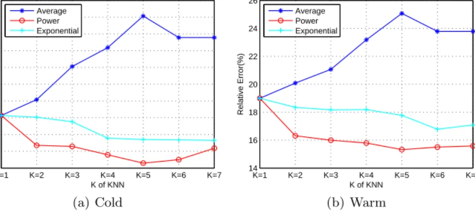
the experiments was the hybrid feature. Table 1 shows the performances of the four models in one-step prediction. SVR models perform poorer than KNN. We investigate this phenomenon and find two possible reasons. One is that the elapsed time has a broad range and SVR considers all the data points in the training set to fit the real value, whereas KNN only considers the points close to the test point. The other reason is that we use mean of actual values in Equation 6, and the values that are far from average will lead to distortion of mean value. Given this result, we chose to use KNN model by default in the following evaluations. K=1 K=2 K=3 K=4 K=5 K=6 K=7 18 19 20 21 22 23 24 25 26 27 28 K of KNN Relative Error(%) Average Power Exponential (a) Cold K=1 K=2 K=3 K=4 K=5 K=6 K=7 14 16 18 20 22 24 26 K of KNN Relative Error(%) Average Power Exponential (b) Warm
Fig. 5.Performance Comparison of Different Weighted KNN Model (One-step)
We evaluated three weighting schemes for KNN regression discussed in Sec-tion 4.2.1, namely Average, Power andExponential. From Figure 5 we observe that the power weighting gives the best performance. In the warm stage, the 15.32% relative error is achieved when K=5. The trend of relative error returns to upward after K=5. Average weighting is the worst weighting method for our data. Exponential weighting does not perform as well as we expected although it is better than average weighting. Weighting schemes show similar performances when the query execution is in the cold stage, i.e., when K=5, the power
weight-ing achieves the lowest relative error of 18.29%. We therefore used K=5 power weighting in following evaluations.
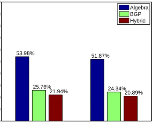
Cold Warm 0 10 20 30 40 50 60 70 80 90 100 53.98% 51.87% 25.76% 24.34% 21.94% 20.89% Relative Error(%) Algebra BGP Hybrid
Fig. 6.Feature Model Selection (One-step)
We also compared the three feature models:Algebra,BGPandHybrid. Figure 6 shows the prediction performance of elapse time on both warm and cold stages. The hybrid feature performs the best and the BGP feature performs better than the algebra feature. Thus we chose hybrid features in following evaluations.
5.3 Performance of Two-Step Regression
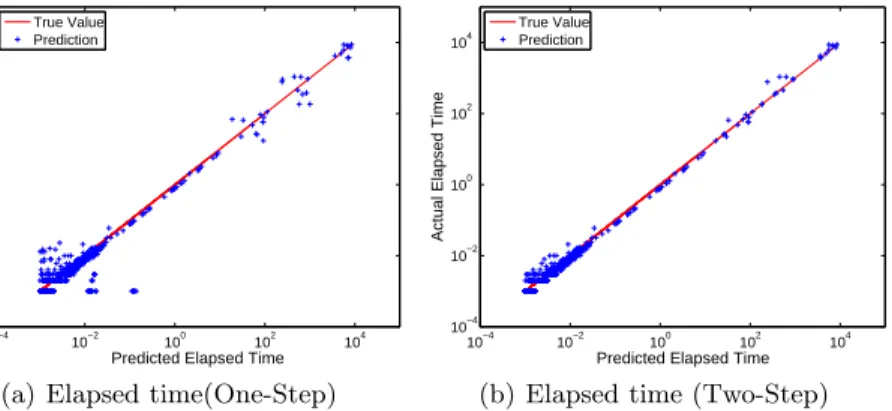
We used SVM for the classification task and achieved accuracy of 98.36%, indi-cating that we can accurately predict the time range. Table 2 shows the result of two-step prediction comparison between KNN and SVR-Polynomial on both warm and cold stage. It shows that SVR regression model still does not perform desirably. It also shows the two-step prediction performs better than one-step prediction. In Figure 7 we compare one-step and two-step prediction on elapsed time in warm stage using log-log plotting.
Table 2. Relative Errors (%) of Two-Step Prediction with KNN and SVR. In the parentheses are the values from one-step prediction
Predictive model Elapsed Time (Cold) Elapsed time (Warm)
5NN(α= 0.3) 11.06(21.94) 9.81(20.89)
10−4 10−2 100 102 104 10−4 10−2 100 102 104
Predicted Elapsed Time
Actual Elapsed Time
True Value Prediction
(a) Elapsed time(One-Step)
10−4 10−2 100 102 104 10−4 10−2 100 102 104
Predicted Elapsed Time
Actual Elapsed Time
True Value Prediction
(b) Elapsed time (Two-Step)
Fig. 7.Elapsed Time Prediction Fitting in Warm Stage(log-log)
5.4 Comparison to the State-of-the-Art
We compare the approach in the work [8] with our approach, as it is the only work that exploits machine learning algorithms to predict SPARQL query. Table 3 shows the result of comparison on warm stage querying. The training time includes feature modelling, clustering and classification for work in [8]. The first part takes the most time because the calculation of GED for all training queries is time-consuming. In our approach (Section 4.1.2), we reduce the GED calculation drastically. But this calculation still takes most time in the prediction process. The time gap of training process between ours and the approach in [8] will be enlarged when more training queries are involved because their approach takes squared time. We do not have clustering process, which further reduces the time used. Our approach also shows better prediction performance with lower relative error for the prediction metric.
Table 3. Comparison to the State-of-the-Art Work. Training time for 1000 queries (Time1k) are compared as well as the relative errors for elapsed time.
Models Time1k Relative Error
Ours SVM+Weighted KNN 51.36 sec 9.81%
[8] X-means+SVM+SVR 1548.45 sec 14.39%
6
Discussions & Conclusion
In this section, we first discuss some observations and issues of this work. Then we conclude this paper.
Plan Features There are two obstacles for using query plan as features in our work. Firstly, this information is based on the cost model estimation, which has been proven as ineffective [2, 6]. Secondly, most of the open source triple stores fail to provide explicit query plans. Thus we turn to choose structure-based features that can be obtained directly from query texts. From our practical experience in this work, we observed that although it leads to distortion of the prediction, the error rate is acceptable based on limited features we can acquire.
Training Size Larger size of the training data would lead to better prediction performance. The reason is that more data variety is seen and the model will be less sensitive to unforeseen queries. However, in practice, it is time consuming to obtain the query elapsed time of a large collection of queries. That is the possible reason why many other works only use small size of queries in their evaluation. This fact will cause the bias of the prediction result and makes similar works hard to compare. Although our experimental query set is larger than theirs, we will consider to further enlarge the size of our query set to cover more various queries in the future.
Dynamic vs Static Data In dynamic query workloads, the queried data is up-dated. Therefore, the prediction might perform poorly due to lack of update of the training data. Our work focuses on prediction on static data and we expect training to be done in a periodical manner. In the future we plan to investigate the techniques to make prediction more available for continuous retraining which reflects recently executed queries.
To conclude, in this paper, we build feature vectors for SPARQL queries by exploiting the syntactic and structural characteristics of the queries. We observe that KNN performs better than SVR on predicting the elapsed time of real-world SPARQL queries. The proposed two-step prediction performs better than one-step prediction because it considers the broad range of observed elapsed time. The prediction in the warm stage is generally better than in the cold stage. We identify the reason comes from same structured queries because many queries are issued by programmatic users, who tend to issue queries using query templates. Our work is on static data and we will consider dynamic workload in the future. Techniques that can incorporate new training data into an existing model will also be considered.
References
1. M. Ahmad, S. Duan, A. Aboulnaga, and S. Babu. Predicting completion times of batch query workloads using interaction-aware models and simulation. InProc. of the 14th International Conference on Extending Database Technology (EDBT 2011), pages 449–460, Uppsala, Sweden, March 2011.
2. M. Akdere, U. C¸ etintemel, M. Riondato, E. Upfal, and S. B. Zdonik.
Learning-based query performance modeling and prediction. In Proc. of the 28th
Interna-tional Conference on Data Engineering (ICDE 2012), pages 390–401, Washington DC, USA, April 2012.
3. N. S. Altman. An Introduction to Kernel and Nearest-Neighbor Nonparametric Regression. The American Statistician, 46(3):175–185, 1992.
4. D. Bursztyn, F. Goasdou´e, and I. Manolescu. Optimizing reformulation-based query answering in RDF. InProc. of the 18th International Conference on Extend-ing Database Technology (EDBT 2015), pages 265–276, Brussels, Belgium, March 2015.
5. C. C. et al. LIBSVM: A library for support vector machines.ACM TIST, 2:27:1–
27:27, 2011.
6. A. Ganapathi, H. A. Kuno, U. Dayal, J. L. Wiener, A. Fox, M. I. Jordan, and D. A. Patterson. Predicting Multiple Metrics for Queries: Better Decisions Enabled
by Machine Learning. In Proc. of the 25th International Conference on Data
Engineering (ICDE 2009), pages 592–603, Shanghai China, March 2009.
7. A. Gubichev and T. Neumann. Exploiting the query structure for efficient join
ordering in SPARQL queries. In Proc. of the 17th International Conference on
Extending Database Technology (EDBT 2014), pages 439–450, Athens, Greece, March 2014.
8. R. Hasan. Predicting SPARQL Query Performance and Explaining Linked Data. In Proc. of the 11th Extended Semantic Web Conference (ESWC 2014), pages 795–805, Anissaras, Crete, Greece, May 2014.
9. J. Li, A. C. K¨onig, V. R. Narasayya, and S. Chaudhuri. Robust Estimation of
Resource Consumption for SQL Queries using Statistical Techniques. The VLDB
Endowment (PVLDB), 5(11):1555–1566, 2012.
10. M. Morsey, J. Lehmann, S. Auer, and A. N. Ngomo. Usage-Centric
Benchmark-ing of RDF Triple Stores. In Proc. of the 26th AAAI Conference on Artificial
Intelligence., Toronto, Canada, July 2012.
11. J. P´erez, M. Arenas, and C. Gutierrez. Semantics and Complexity of SPARQL.
ACM Transactions on Database Systems, 34(3), 2009.
12. A. Rajaraman and J. D. Ullman.Mining of Massive Datasets. Cambridge
Univer-sity Press, 2011.
13. A. Smola and V. Vapnik. Support Vector Regression Machines.Advances in neural
information processing systems, 9:155–161, 1997.
14. M. Stocker, A. Seaborne, A. Bernstein, C. Kiefer, and D. Reynolds. SPARQL
Basic Graph Pattern Optimization Using Selectivity Estimation. In Proc. of the
17th International World Wide Web Conference (WWW 2008), pages 595–604, Beijing, China, April 2008.
15. P. Tsialiamanis, L. Sidirourgos, I. Fundulaki, V. Christophides, and P. A. Boncz.
Heuristics-based query optimisation for SPARQL. In Proc. of the 15th
Interna-tional Conference on Extending Database Technology (EDBT 2012), pages 324– 335, Uppsala, Sweden, March 2012.
16. W. Wu, Y. Chi, S. Zhu, J. Tatemura, H. Hacig¨um¨us, and J. F. Naughton.
Pre-dicting query execution time: Are optimizer cost models really unusable? InProc. of the 29th International Conference on Data Engineering (ICDE 2013), pages 1081–1092, Brisbane Australia, April 2013.
17. X. Wu, V. Kumar, J. R. Quinlan, J. Ghosh, Q. Yang, H. Motoda, G. J. McLachlan, A. F. M. Ng, B. Liu, P. S. Yu, Z. Zhou, M. Steinbach, D. J. Hand, and D. Steinberg.
Top 10 algorithms in data mining. Knowledge and Information Systems, 14(1):1–