Segmentation with Auxiliary
Information
Tao Wang
A thesis submitted for the degree of
Doctor of Philosophy
of The Australian National University
November 2016
c
Copyright by Tao Wang 2016
Although supervisors always play an instrumental role in one’s journey towards thesis com-pletion, I believe my own supervisors, Xuming He and Nick Barnes, deserve a very special mention for their continual encouragement, exceptional guidance and unwavering support over the years. I am deeply indebted to Xuming, for his dedication and understanding in vision and learning opened up a whole new world for me. Xuming has always been a role model, a caring mentor and a close friend of mine. I want to thank him for encouraging me develop a well-rounded understanding of the problems I wanted to tackle, for providing very practical guidance while it was difficult to make progress, and for repeatedly helping me with presenting my findings in a logical and lucid manner. It is fair to say that I would not be who I am now had I not worked with him. I am deeply grateful to Nick, for the countless times of inspiring and encouraging discussions, for the many insightful ideas he contributed, and also for tirelessly fixing imperfections in my presentations and writings. It has been a privilege and an infinite source of gratitude to be guided by Nick who has always been understanding and supportive throughout my study.
I would like to extend my sincerest thanks to my supervisory panel, Chunhua Shen and Richard Hartley for their sound advice and thought-provoking questions. In particular, I have learned a great deal from discussions with Chunhua in the first year of my study. I also appre-ciate his encouragement and support while I write up my thesis. Furthermore, I am fortunate to have been a member of the BVA vision processing team, the NICTA computer vision re-search group and the broader ANU vision and robotics group. I have immensely benefited from seminars, summer schools and other group activities which allow me to meet and learn from students and scholars from around Australia. I want to especially thank Hanxi Li, Miao-miao Liu and Mathieu Salzmann for the excellent discussions and enlightenment in our weekly reading groups. In addition, I want to thank NICTA’s Intelligent Transport Systems project for providing me an opportunity to work as a part-time research programmer.
I also want to thank my lab mates for their many insightful ideas on my thesis project, their company, and friendship: Buyu Liu, Lin Gu, Fang Wang, Weipeng Xu, Wei Zhuo, Zongyuan Ge, Zeeshan Hayder, Lachlan Horne, Samunda Perera, David Feng, Kyoungup Park, Zhihui Hao, Cong Phuoc Huynh. . . The days we worked in the same lab and the happy times we spent together in the beautiful landscapes of Canberra have been seared in my memory.
Last but not least, thank all my friends outside my academic life. Thanks to my parents, for their life-long love and encouragement.
One fundamental problem in computer vision and robotics is to localize objects of interest in an image. The task can either be formulated as an object detection problem if the objects are described by a set of pose parameters, or an object segmentation one if we recover object boundary precisely. A key issue in object detection and segmentation concerns exploiting the spatial context, as local evidence is often insufficient to determine object pose in the presence of heavy occlusions or large object appearance variations. This thesis addresses the object detection and segmentation problem in such adverse conditions with auxiliary depth data pro-vided by RGBD cameras. We focus on four main issues in context-aware object detection and segmentation: 1) what are the effective context representations? 2) how can we work with limited and imperfect depth data? 3) how to design depth-aware features and integrate depth cues into conventional visual inference tasks? 4) how to make use of unlabeled data to relax the labeling requirements for training data?
We discuss three object detection and segmentation scenarios based on varying amounts of available auxiliary information. In the first case, depth data are available for model training but not available for testing. We propose a structured Hough voting method for detecting objects with heavy occlusion in indoor environments, in which we extend the Hough hypothesis space to include both the object’s location, and its visibility pattern. We design a new score function that accumulates votes for object detection and occlusion prediction. In addition, we explore the correlation between objects and their environment, building a depth-encoded object-context model based on RGBD data. In the second case, we address the problem of localizing glass objects with noisy and incomplete depth data. Our method integrates the intensity and depth information from a single view point, and builds a Markov Random Field that predicts glass boundary and region jointly. In addition, we propose a nonparametric, data-driven label trans-fer scheme for local glass boundary estimation. A weighted voting scheme based on a joint feature manifold is adopted to integrate depth and appearance cues, and we learn a distance metric on the depth-encoded feature manifold. In the third case, we make use of unlabeled data to relax the annotation requirements for object detection and segmentation, and propose a novel data-dependent margin distribution learning criterion for boosting, which utilizes the in-trinsic geometric structure of datasets. One key aspect of this method is that it can seamlessly incorporate unlabeled data by including a graph Laplacian regularizer. We demonstrate the performance of our models and compare with baseline methods on several real-world object detection and segmentation tasks, including indoor object detection, glass object segmentation and foreground segmentation in video.
Several contributions presented in this thesis have been published elsewhere by the author. We list these below:
• Chapter 3 - Structured Hough Voting for Joint Object Detection and Occlusion Prediction:
Tao Wang, Xuming He and Nick Barnes, ‘Learning Structured Hough Voting for Joint Object Detection and Occlusion Reasoning’, InProceedings of IEEE International Con-ference on Computer Vision and Pattern Recognition (CVPR 2013), Portland, USA, 2013.
• Chapter 4 - Glass Object Segmentation by Joint Inference of Boundary and Depth: Tao Wang, Xuming He and Nick Barnes, ‘Glass Object Localization by Joint Inference of Boundary and Depth’, InProceedings of IEEE International Conference on Pattern Recognition (ICPR 2012), Tsukuba, Japan, 2012.
• Chapter 5 - Glass Object Segmentation by Label Transfer on Joint Depth and Ap-pearance Manifolds:
Tao Wang, Xuming He and Nick Barnes, ‘Glass Object Segmentation by Label Trans-fer on Joint Depth and Appearance Manifolds’, InProceedings of IEEE International Conference on Image Processing (ICIP 2013), Melbourne, Australia, 2013.
• Chapter 6 - Laplacian Margin Distribution Boosting for Learning from Sparsely Labeled Data:
Tao Wang, Xuming He, Chunhua Shen, Nick Barnes, ‘Laplacian Margin Distribution Boosting for Learning from Sparsely Labeled Data’, InProceedings of IEEE Interna-tional Conference on Digital Image Computing: Techniques and Applications (DICTA 2011), Noosa, Australia, 2011.
Acknowledgments v
Abstract vii
Publications ix
1 Introduction 1
1.1 Our research problems . . . 4
1.2 Object detection with depth-encoded context . . . 6
1.3 Glass segmentation by joint inference of boundary and region . . . 8
1.4 Depth-aware features and label transfer . . . 9
1.5 Learning from sparsely labeled data . . . 11
1.6 Thesis outline . . . 11
1.7 Major contributions . . . 13
2 Literature Review 15 2.1 Object detection in computer vision . . . 15
2.1.1 Sliding window detectors . . . 16
2.1.2 Hough transform detectors . . . 20
2.1.3 Object detection with RGBD data . . . 27
2.1.4 Occlusion reasoning for object detection . . . 28
2.1.5 Context modeling for object detection . . . 31
2.2 Object segmentation in computer vision . . . 33
2.2.1 Foreground object segmentation . . . 34
2.2.2 Context modeling with Markov Random Fields . . . 36
2.2.3 Inference in Markov Random Fields . . . 41
2.2.4 Glass object segmentation . . . 43
2.3 Boosting for learning from sparsely labeled data . . . 47
2.4 Summary . . . 51
3 Structured Hough Voting for Joint Object Detection and Occlusion Prediction 53 3.1 Introduction . . . 53
3.2 Our approach . . . 55 xi
3.2.1 Structured Hough voting . . . 55
3.2.2 Depth-encoded context . . . 58
3.2.2.1 Second-order features . . . 59
3.3 Model learning and inference . . . 60
3.3.1 Joint inference for object detection and occlusion prediction . . . 60
3.3.2 Learning with depth-augmented data . . . 62
3.4 Experimental evaluation . . . 63
3.4.1 Dataset and setup . . . 63
3.4.2 Model details . . . 64
3.4.3 Quantitative results . . . 64
3.4.4 Segmentation performance analysis . . . 67
3.4.5 More detailed examples . . . 68
3.5 Conclusion . . . 69
4 Glass Object Segmentation by Joint Inference of Boundary and Depth 77 4.1 Introduction . . . 77
4.2 Our approach . . . 79
4.2.1 Boundary and region graph . . . 79
4.2.2 A Markov Random Field on boundaries and superpixels . . . 83
4.2.3 Joint prediction . . . 87
4.2.4 Depth reconstruction . . . 89
4.3 Experimental evaluation . . . 89
4.3.1 Dataset and setup . . . 89
4.3.2 Recall statistics for glass proposal . . . 89
4.3.3 Segmentation results and comparisons . . . 91
4.3.4 Qualitative analysis for joint inference . . . 93
4.4 Conclusion . . . 95
5 Glass Object Segmentation by Label Transfer on Joint Depth and Appearance Manifolds 99 5.1 Introduction . . . 99
5.2 Our approach . . . 101
5.2.1 Superpixels and features . . . 101
5.2.2 Boundary label transfer . . . 102
5.2.3 Object model and inference . . . 103
5.3 Experimental evaluation . . . 104
5.3.1 Data specifications and setup . . . 104
5.3.3 Results and discussion . . . 107
5.3.4 Building subset-specific manifolds . . . 109
5.4 Conclusion . . . 111
6 Laplacian Margin Distribution Boosting for Learning from Sparsely Labeled Data115 6.1 Introduction . . . 115
6.2 Our approach . . . 117
6.2.1 Margin distribution and Laplacian MDBoost . . . 117
6.2.2 Semi-supervised Laplacian MDBoost . . . 119
6.3 Experimental evaluation . . . 121
6.3.1 Datasets and setup . . . 122
6.3.2 Laplacian MDBoost for supervised learning . . . 123
6.3.3 Semi-supervised Laplacian MDBoost . . . 124
6.3.4 Video segmentation with Semi-supervised Laplacian MDBoost . . . . 125
6.3.5 RGBD glass object segmentation with Semi-supervised Laplacian MD-Boost . . . 126
6.4 Conclusion . . . 128
7 Conclusion 135 7.1 Primary contributions . . . 135
7.2 Future work . . . 137
7.2.1 3D scene structure reasoning . . . 137
7.2.2 Holistic scene understanding . . . 138
7.2.3 Other types of auxiliary information . . . 138
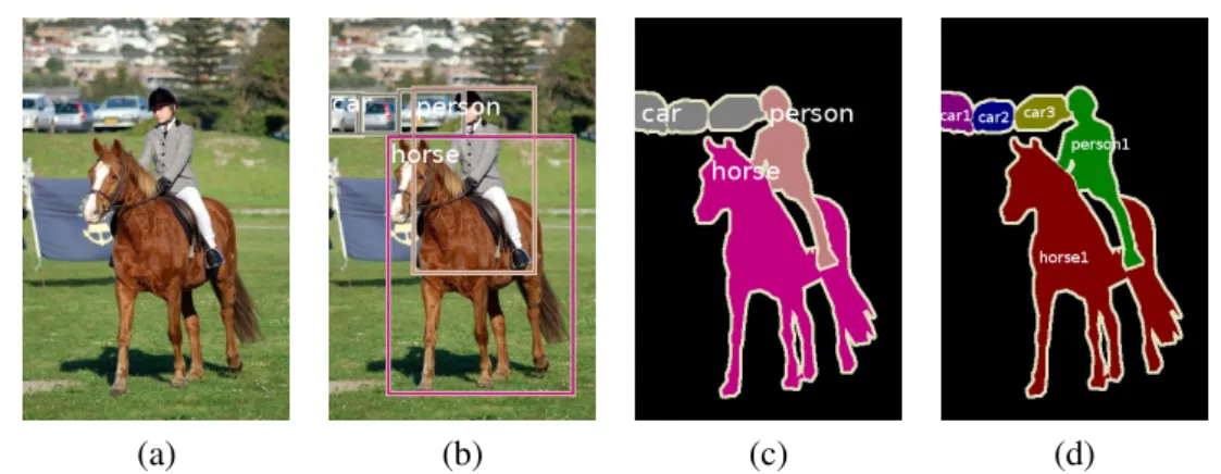
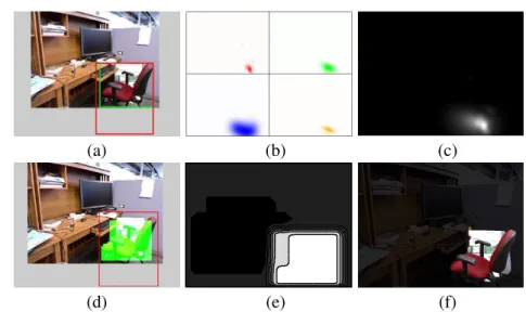
1.1 Example of object detection and segmentation. (a) input image. (b) object detection with bounding boxes. (c)semantic segmentation.(d)object instance segmentation. . . 2 1.2 Illustration of the proposed object detector. (a)RGB frame with object
bound-ing box (red) and visible part boundbound-ing box (green). (b)Object centroid voting from multiple layers. (c)Combined object centroid voting results. (d) Detec-tor output (red) with visibility pattern prediction (green). (e)Object visibility pattern prediction results.(f)Final segmentation results. . . 7 1.3 Illustration of the proposed glass object segmentation system. (a) Intensity
image with ground truth foreground mask overlaid. (b)Edge detector output. (c)Triangulation result.(d)Boundary classifier output (magnified).(e) Super-pixel classifier output (magnified).(f)Reconstructed depth with joint inference result overlaid. . . 8 1.4 Top: Illustration of feature manifold based glass boundary classification. We
use a learned feature manifold to match every boundary fragment in a test scene (shown as image patches) to training set in order to predict its label. Bottom: Large variation on glass boundaries: patches examples. . . 10 2.1 Visualization of HOG feature space.(a)input image.(b)HOG cells and local
gradient orientations.(c)A visualization of HOG features using method in [208]. 17 2.2 Example of RGBD imagery. The point cloud was reconstructed from a video
sequence including the color and depth frames. Depth images are color coded so that pixels close to the camera are shown in blue, and far-away pixels are in red. Missing depth values are shown in white. . . 27 2.3 The frontal views of two visually similar chairs (cropped). For each chair the
original image is shown on the left ((a) and(c) ), with the visualized HOG feature map [208] on the right ((b)and(d)). For the partially occluded chair, the seat and the base are occluded by a table in the front. See text for details. . . 29 2.4 Example of indoor scenes. Note how objects are occluded or truncated by
image boundaries. Groups of objects are also arranged together to facilitate human interactions. . . 31
2.5 Two examples of neighborhood graphs for Markov Random Fields.Left Panel: A 4-connected grid of image pixels.Right Panel:An 8-connected grid of im-age pixels. . . 36 2.6 The factor graph of the pairwise MRF in Equation 2.20. For simplicity, only
three nodes are shown. . . 37 2.7 Example of image labeling results with TextonBoost [185] using unary terms
only, and with pairwise terms added. (a)input image. (b)ground-truth label-ing. (c)image labeling result with unary terms only. (d)image labeling result with pairwise terms added. . . 40 2.8 Example RGBD image pairs containing glass objects. Note the distinctive but
irregular missing patterns in and around glass regions. See text for details. . . . 44 3.1 Illustration of structured Hough voting. (a)RGB frame with object bounding
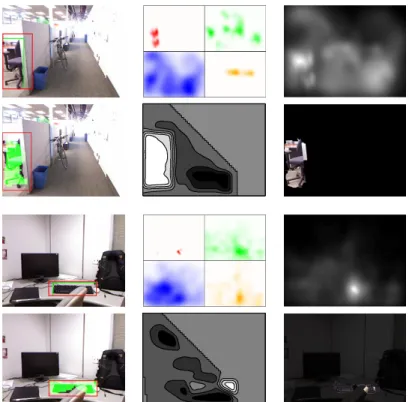
box (red) and visible part bounding box (green). (b)Object centroid voting from multiple layers. (c)Combined object centroid voting results. (d) Detec-tor output (red) with visibility pattern prediction (green). (e)Object visibility pattern prediction results.(f)Final segmentation results. . . 54 3.2 Top-ranked clusters (presented with the patches closest to the cluster centers)
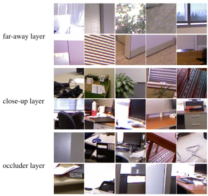
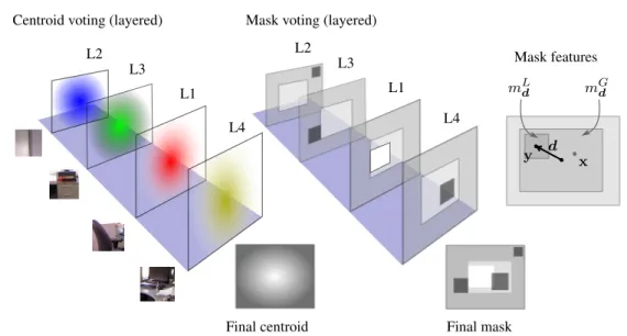
for 3 contextual layers on the Berkeley 3D object dataset. . . 55 3.3 Illustration of multiple layered object centroid and mask voting. L1
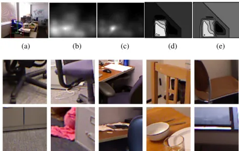
corre-sponds to the object layer, and L2, L3, L4 correspond to far-away context, close-up context and occluder layers, respectively. For mask voting, brighter regions indicate a higher response, while darker regions indicate a lower re-sponse. . . 56 3.4 Illustration of the impact of patch pair terms on hypothesis scoring. Upper
panel: A specific example, with (a)RGB frame with an example of a patch pair (in blue rectangles). (b)Object centroid voting results without patch pair terms.(c)Object centroid voting results with patch pair terms added.(d)Shape voting results without patch pair terms.(e)Shape voting results with patch pair terms added. Lower panel: The highest ranked patch pairs on the Berkeley 3D object dataset. The first row shows on-object patches, and the second row shows off-object patches. Each column corresponds to a patch pair. . . 59 3.5 An illustration of how iterative inference updates the object centroid and
sup-porting mask hypotheses. The first row on the right shows object centroid vot-ing, with the corresponding supporting mask estimations shown in the second row. . . 62 3.6 Detection examples of our approach. See text for details. . . 65
3.7 Detection precision-recall curves on the Berkeley 3D Object dataset (left) and the NYU Depth dataset (right). The solid curve corresponds to our approach (Ours). The dashed curves correspond to baseline methods: Deformable Parts Model (DPM) [46], Max-margin Hough transform (M2HT) [129], and Max-margin Hough transform with 2D geometric context (2D). See details in text.
. . . 66 3.8 Detection precision-recall curves on the Berkeley 3D Object dataset (left) and
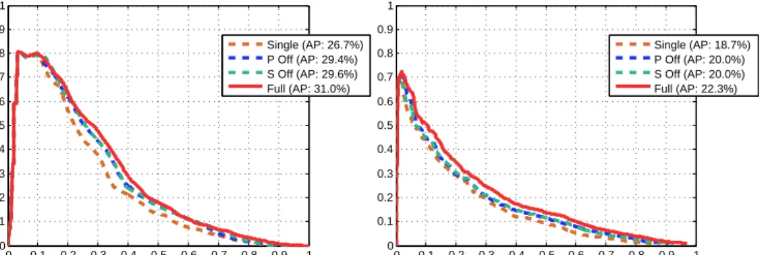
the NYU Depth dataset (right). The solid curve corresponds to our full model (Full). The dashed curves correspond to diagnostic results with various com-ponents in our full model turned off, i.e., single layer context (Single), patch pair term off (P Off), and segmentation off (S Off). See details in text. . . 66 3.9 Precision-recall curves on the Berkeley 3D Object dataset (left) and the NYU
Depth dataset (right) for segmentation at50%recall rate in Figure 5.5. Simul-taneously voting for local feature position and whole object hypothesis yields the best segmentation results. . . 68 3.10 More experimental results of the proposed approach on Berkeley 3D Object
Dataset [77] and NYU Depth Dataset [145]. Each row corresponds to a specific instance on a test image. See text for detailed discussion. . . 69 3.11 Per-class detection precision-recall curves on the Berkeley 3D Object dataset
(B3DO). The solid curve corresponds to our approach (Ours). The dashed curves correspond to baseline methods: Deformable Parts Model (DPM) [46], Max-margin Hough transform (M2HT) [129], and Max-margin Hough trans-form with 2D geometric context (2D). See details in text. . . 71 3.12 Per-class detection precision-recall curves on the NYU Depth dataset (NYU).
The solid curve corresponds to our approach (Ours). The dashed curves corre-spond to baseline methods: Deformable Parts Model (DPM) [46], Max-margin Hough transform (M2HT) [129], and Max-margin Hough transform with 2D geometric context (2D). See details in text. . . 72 3.13 Per-class detection precision-recall curves on the Berkeley 3D Object dataset
(B3DO). The solid curve corresponds to our full model (Full). The dashed curves correspond to diagnostic results with various components in our full model turned off, i.e., single layer context (Single), patch pair term off (P Off), and segmentation off (S Off). See details in text. . . 73 3.14 Per-class detection precision-recall curves on the NYU Depth dataset (NYU).
The solid curve corresponds to our full model (Full). The dashed curves cor-respond to diagnostic results with various components in our full model turned off, i.e., single layer context (Single), patch pair term off (P Off), and segmen-tation off (S Off). See details in text. . . 74
4.1 Illustration of the proposed approach. (a) Intensity image with ground truth foreground mask overlaid. (b)Edge detector output. (c)Triangulation result. (d) Boundary classifier output (magnified). (e) Superpixel classifier output (magnified). (f)Reconstructed depth with joint inference result overlaid. . . 78 4.2 Examples of the boundary and region graph construction. (a)Input intensity
image.(b)Input depth image (missing readings are shown in white).(c)Glass region proposal with proposed glass regions in black.(d)Triangulation result. . 80 4.3 An example of boundary proposal including glass, depth and RGB boundary.
(a) BGTG boundary detector output. (b) Glass region proposal results. (c) depth boundary detector output before alignment.(d)low-threshold RGB edge detector output. See text for details. . . 81 4.4 The factor graph of the MRF model for our glass detector. Each black square
represents a term in Equation 5.2. Each circular node represents a random variable. Shaded nodes are observations. . . 83 4.5 Illustration of our angle preference for boundary pairwise term. In the top
and middle examples, the angles between connected boundary fragments are obtuse and straight respectively. These are commonly found in ground-truth glass boundaries. In the bottom example, however, the angle is acute and is more likely a result from incorrectly identified glass boundary. . . 86 4.6 Illustration of our superpixel pairwise term. Assume the arrow points towards
glass regions in red, and the non-glass regions are in blue. See text for details. 87 4.7 The precision-recall curves based on boundary matching (left panel) and
pix-elwise region matching (right panel). . . 91 4.8 Examples of glass detection results on our new RGBD Glass dataset. Note
that missing areas are shown in white, and depth readings are recovered by a piece-wise planar model. . . 93 4.9 Failure examples of glass detection on our RGBD Glass dataset. See text for
details. . . 94 4.10 Examples of boundary and region unary terms (magnified, the viewing window
is marked as a red bounding box in the RGB images). The boundary orienta-tion is shown as a red arrow pointing towards glass regions. Local boundary and region classifiers provide complementary information for glass object seg-mentation. See text for details. . . 96 4.11 Examples of iterative joint inference. While the initial boundary inference
smoothes the unary classifier output, we obtain much cleaner boundary infer-ence results with the joint inferinfer-ence. See text for details. . . 97
5.1 Top: Illustration of feature manifold based glass boundary classification. We use a learned feature manifold to match boundary fragments in a test scene (shown as image patches) to a training set in order to predict their labels. Bot-tom:Large variation on glass boundaries: patches examples. . . 100 5.2 Example of SLIC [2] superpixels with initial region sizes of 10px (left) and
30px (right) respectively. . . 102 5.3 Example images from the three subsets of our RGBD Glass dataset. See text
for details. . . 105 5.4 Qualitative comparisons between triangulation-based image partitioning method
(left two columns, partitions shown in orange) used in Chapter 4 and SLIC [2] superpixels (right two columns, partitions shown in red). Note how SLIC su-perpixels more closely follow glass boundaries, especially in regions high-lighted with blue circles. The SLIC initial region size shown here is 10 px.
. . . 106 5.5 The overall precision and recall on RGBD Glass dataset for various methods.
Left: Performance based on boundary pixel accuracy. Middle: Performance based on region pixel accuracy on the whole dataset. Right: Performance based on region pixel accuracy in the glass boundary neighborhoods (i.e., re-gions within10px of ground-truth glass boundaries). . . 112 5.6 Hard examples of glass detection results on the RGBD glass dataset. Column
(a): RGB image frame.(b): Unary responses from local glass boundary classi-fiers in Chapter 4.(c): Joint inference and depth recovery results in Chapter 4. (d): Glass boundary label transfer results. (e): Inference and depth recovery results with the proposed method. Note that missing depth readings are recov-ered by a piece-wise planar model for glass region and smoothed out using a median filter elsewhere. . . 113 5.7 Normalized accumulated weight for different features on the RGBD Glass
dataset (All) and its subsets (Floor, Laboratory and Office). We add up the absolute values of weights for feature dimensions belong to specific types of features. The resulting bar graph illustrates the relative accumulated “impor-tance” of various types of features used in our method. The feature types are: Hue and Saturation (HS), Blurring (Blur), Blending and Emission (BE), Tex-ture Distortion (TexTex-ture), Missing Depth (Missing), Color histogram (Color), HOG on depth data (HOD), Range histogram (Range). See text for details. . . 114 6.1 Examples of different choices of the edge weightswij for the graph Laplacian.
6.2 Average test errors (with standard deviations) of AdaBoost, AdaBoost-CG, LPBoost, MDBoost and Laplacian MDBoost on13UCI benchmark datasets. . 130 6.3 Performance of Laplacian MDBoost (dash-dot line) and Semi-supervised
Lapla-cian MDBoost (solid line) on UCI datasetsbanana(green),ringnorm(blue) andsplice(red). . . 131 6.4 Examples of video segmentation with three different semi-supervised
algor-ithms: Semi-supervised Laplacian MDBoost (SemiLap-MDBoost), Learning with local and global consistency combined with MDBoost (LLGC+MDBoost) and SemiBoost. The video data are sequences0370and0950from the Youtube Celebrity Face Tracking and Recognition Dataset [83]. . . 132 6.5 Examples of coarse ground-truth superpixel labelings used for our glass region
classification experiment. Each red bounding box covers a ground-truth glass object. The center-aligned green bounding boxes cover one fourth the area of the red bounding boxes. A superpixel is labeled as glass if it has50%or more overlap with the green bounding box, and non-glass if it has 50% or more overlap with the region outside the red bounding box. All superpixels inside the red bounding box but outside the green bounding box are treated as unlabeled data. See text for details. . . 133
3.1 Per-class average precision on the Berkeley 3D Object dataset and the NYU Depth dataset. Mean average precision values are calculated separately for each dataset. . . 75
4.1 The overall glass region recall rate, near-boundary glass region recall rate, and the proposed glass area under different dilation disk radiir. Settingr= 15px gives a good tradeoff between recall rates and the proposed area. See text for details. . . 90 4.2 The glass boundary recall rates from various boundary cues. The first three
columns give the recall rates for the three boundary cues in Equation 4.1. The last two columns give the recall rates using the combination of the three cues, before and after triangulation. See text for details. . . 91 4.3 F-measures at50% recall for boundary and region accuracy metrics,
respec-tively. . . 91 4.4 Comparison of average runtime per image (in seconds) between detached and
joint inference. The numbers report here are a comparison of MRF inference times (not including feature extraction and local classification). . . 92
5.1 Glass boundary recall rates for triangulation-based method used in Chapter 4 versus SLIC [2] used in this chapter. emax denotes the pixel error tolerance. See text for details. . . 106 5.2 Precision (in percentage%) and F-measures at25%,50%and75%recall for
glass boundary label transfer. Column Base refers to baseline performance without the feature pool. Columns (1) through (3) refer to (1) image parti-tioning at multiple scales, (2) sampling features on multiple scales, and (3) sampling features at multiple locations. Column Full refers to our full model with all of the three components. See text for details. . . 107
5.3 Precision (in percentage%) and F-measures at25%,50%and75%recall for glass boundary label transfer. The first three columns refer to scenarios in which we remove certain depth-aware features. Specifically, they refer to No Color histogram (NC), No HOG on depth data (NH) and No Range histogram (NR), respectively. The fourth column,kNN, refers to the case where we dis-able the distance metric learning. The final column, Full, refers to our full model. See text for details. . . 107 5.4 F-measures at50%recall for boundary and region accuracy metrics. The final
row (Bound Region) is based on region pixel accuracy in the glass boundary neighborhoods (i.e., regions within10px of ground-truth glass boundaries). . . 108 5.5 Per-image runtime statistics for the method in Chapter 4 and the proposed
method. On average the proposed method is about 8 times faster. See text for details. . . 108 5.6 Precision (in percentage %) at 25%, 50%and 75%recall for glass boundary
label transfer on the three subsets of our RGBD Glass dataset. Columns under “Single manifold” refer to results from our proposed approach with a single manifold built on the entire dataset. Columns under “Subset-specific manifold” refer to results obtained with subset-specific manifolds. . . 110 6.1 Test error and standard deviation (in percentage %) of Laplacian MDBoost
(using only labeled data), Semi-supervised Laplacian MDBoost (SemiLap-MDBoost), Learning with Local and Global Consistency combined with MD-Boost (LLGC+MDMD-Boost), and SemiMD-Boost on UCI datasets. . . 124 6.2 Average test and training error (in percentage%) of Semi-supervised Laplacian
MDBoost (SemiLap-MDBoost), Learning with Local and Global Consistency combined with MDBoost (LLGC+MDBoost), and SemiBoost on the YouTube Celebrities Face Tracking and Recognition Datasets over10tests. . . 126 6.3 Precision (in percentage%) at25%,50%and75%recall for glass region and
boundary classification using fully labeled dataset and partially labeled dataset, respectively. Methods using fully labeled dataset include SVM and Random Forest (RF) from Chapter 4 and MDBoost. Methods using partially labeled dataset include Laplacian MDBoost (without using unlabeled data), Semi-supervised Laplacian MDBoost (SemiLap-MDBoost), Learning with Local and Global Consistency combined with MDBoost (LLGC+MDBoost), and SemiBoost. . . 128
Introduction
One fundamental problem in computer vision and robotics is to make computers capable of understanding three-dimensional scenes from visual information. Such capacity is one of the most impressive features of the human visual system: we all have the ability to quickly, ac-curately and comprehensively interpret the visual world. The various tasks involved here are referred to asscene understandingin computer vision. Broadly speaking, scene understanding aims at resolving the gap between low level image features and high level semantic concepts. One of the core problems here is to localize objects of interest. Take the picture in Figure 1.1 (a) for example, a human can effortlessly (1) recognize the person, the horse, and the cars in the picture, and (2) delineate where these objects are.
These abilities give rise to two popular paradigms for localizing objects in computer vi-sion, i.e.,object detectionandobject segmentation. Both tasks involve inferring the location of objects belonging to a specific category from an image with different levels of details. Object detection, as depicted in Figure 1.1 (b), parametrizes object location with a rectangular bound-ing box. The boundbound-ing box has an associated category label (e.g., person, horse, or car) and optional pose parameters (e.g., frontal-view, rear-view or side-view for cars). Object segmen-tation, as depicted in Figure 1.1 (c), is more accurate in the sense that it computes a pixelwise segmentation for the objects. The segmentation may additionally identify individual object instances as shown in Figure 1.1 (d), because multiple object instances belonging to the same category may spatially overlap.
Being able to localize objects is an essential functionality for many real-world applications including autonomous vehicles, content-based image search, event detection in video surveil-lance, inspection and quality control, etc. In general, localizing objects is arguably one of the most essential steps towards understanding a scene, and it opens the possibility for interacting with identified objects in the environment. In particular, object detection and segmentation link together the semantics and the geometry of a scene, which means it has close ties with other scene understanding problems in computer vision such as image classification and geometry estimation.
Although localizing objects seems to be an effortless task for humans in most cases, it 1
(a) (b) (c) (d)
Figure 1.1: Example of object detection and segmentation. (a)input image. (b)object detec-tion with bounding boxes.(c)semantic segmentation.(d)object instance segmentation. remains perhaps one of the most challenging problems in computer vision. The challenging nature of this problem lies in the fact that objects in realistic settings exhibit considerable in-traclass appearance variability due to multiple factors such as occlusion, viewpoint variations, and background clutter. In addition, more image data obtained in unstructured environment are constantly being created as low-cost consumer cameras become ubiquitous. There has been an increasing number of pictures taken in cluttered environments from more arbitrary viewpoints, with many potentially interesting objects being only partially visible. These objects would adversely affect both the training and the evaluation of object detection and segmentation alg-orithms due to their large appearance variations.
In face of the problem, the visual information from a single color image may be insuffi-cient for computers to localize challenging object classes. In fact, information in the real world comes through multiple input modalities, and we may utilize auxiliary input to explain away some of the ambiguities in color images. The benefit of learning to localize objects with multi-modal input is at least threefold. Firstly, different multi-modalities may exhibit distinct statistical properties due to the underlying fact that they typically carry different kinds of information. This allows us to discover useful information about the objects and the scene. For example, we may consider the auxiliary information provided by a textual input modality, which may provide concepts such as the psychological perception of an object (e.g., beautiful, interesting, valuable) that is usually not obvious from visual information. As an another example, one par-ticular problem in 2D imaging is that it is challenging to infer 3D configurations of the objects and the scene from a single color image. Without a depth estimation, it requires a lot of effort to manually label the 3D configurations of objects and their parts. Therefore we may consider the multi-modal input provided by depth-capable cameras. For example, the RGBD cameras such as Kinect can collect high quality depth maps and registered color images for indoor envi-ronments. The depth maps provide a 2.5D point cloud representation of the scene from which we may infer credible cues for the underlying 3D geometry. Secondly, we may learn joint
representations by fusing data from different modalities to capture real-world concepts and re-solve ambiguities. Take depth maps again as an example, they encode useful information about the interactions between an object and its environments, such as the distance between two ob-jects and the occlusion relationships. This allows us, for example, to learn a depth-encoded object appearance model. In addition, we may build a joint feature representation with better class separability by including depth-aware features. Lastly, an important finding from our work is that learning an object model with multimodal input helps even when some modalities are absent during model evaluation. This opens up a new perspective to localizing objects in which we use auxiliary information to help us train a better object model, and apply the model to a test setting where the auxiliary information may be unavailable. Similar ideas have also been suggested in both the psychological [181] and computer vision [191, 32, 22, 186, 234] communities.
In this thesis, we make use of auxiliary information to build object detection and segmen-tation algorithms, with a focus on modeling the object and its environments with multi-modal input generated from RGBD cameras. We discuss both generic object detection and semi-transparent object (e.g., glass) segmentation. The latter is a specific type of objects which lacks homogeneity of surface appearance and therefore requires purposely designed features and inference algorithms. It should also be noted that the amount of available depth data may vary in practice. For instance, the majority of cameras equipped on handheld devices today do not come with a depth sensor. Therefore, assuming depth maps as a part of an algorithm’s input may limit its applicability. This reality prompts us to train an object model with auxil-iary depth information and to test without depth maps as discussed. In addition, we address a general problem in object detection and segmentation that it is expensive to obtain precise and complete ground-truth for large datasets. More specifically, we address the four primary challenges as follows:
1)Partial object observation.Localizing objects remains challenging for cluttered/crowded scenes, such as indoor environments, where objects are frequently occluded by neighboring objects or the viewing window. The partial objects being observed usually provide limited information on the object position and pose, so many previous object detection approaches are prone to failure as they solely rely on image cues from objects themselves. In this regard, it is important to seek additional information from the environment. Specifically, the availabil-ity of depth imagery enables modeling the environment in 3D. Depth maps can provide direct evidence to resolve the ambiguities resulting from projecting the underlying 3D world to a 2D image. In particular, occlusion can be viewed as a special type of contextual relationship in 3D, which would become an intrinsic component of object and scene models.
2)Partial sensory data. Localizing semi-transparent objects from a single color image is challenging due to lack of locally discriminative visual features and homogeneity of surface appearance. Therefore, the auxiliary information such as depth maps can be an important cue
for localizing these objects. However, depth maps provided by RGBD cameras are imperfect in the sense that they may contain incorrect or missing readings due to various local refractive properties of the structured light being projected. Therefore, it is important for our algorithms to adapt to the imperfections and counter their negative impact. In addition, we can improve depth reconstruction of the scene if we are able to partially correct the artefacts in depth maps. 3)Fusing data from different modalities. It is a non-trivial issue to fuse data from dif-ferent modalities, e.g., to integrate depth cues into conventional visual inference tasks. The integration can happen at different granularities such as either at the local image patch level or the object and scene level. It could also happen at various stages of the algorithm such as either during feature extraction or model inference. Therefore, the integration of data from multiple modalities is an important aspect of our methods.
4)Partial ground-truth annotation.Auxiliary information can also be provided by unla-beled data. By designing a semi-supervised learning algorithm, we are able to work with large datasets with only a fraction of images labeled. In addition, we may also relax the labeling requirements for object segmentation. For example, we can train algorithms with coarse labels (e.g., an object bounding box) without the need to specify exact object boundaries. In fact, a generic semi-supervised learning technique can be applied to a range of real-world applications that involve a classification problem.
In the following section, we discuss four specific research problems raised in this thesis, addressing the primary challenges above. In Sections 1.2 to 1.5, we outline the main ideas of our work in response to the research problems. Section 1.6 summarizes the content of each chapter, and Section 1.7 lists the major contributions from this thesis.
1.1
Our research problems
To reliably detect or segment objects in the presence of background clutter and heavy occlu-sion, and in order to address different levels of auxiliary information availability, we provide solutions to the following four central research problems in this thesis:
1)Depth-aware context modeling. In each image, the structural prior information of its scene essentially defines acontext1. For a single intensity image, an important class of context is the two-dimensional projection of 3D scenes. Co-registered RGBD imagery allows for mod-eling contextual elements in the underlying 3D world. Context reasoning can be carried out at multiple levels. We can discard relative geometric relationships between objects and context and describe context at a geometry-free level, e.g., the presence of a table in an image raises our expectation of seeing chairs. By encoding the relative geometric distributions between ob-jects and context, we are able to provide more specific cues, e.g., the vicinity of a table is more
1
There are many sources of contextual information (e.g., spatial context, semantic context and temporal con-text). In this thesis we focus on the spatial context. See [40] for details on various sources of contextual information.
likely to contain chairs. Another option is to discard the notion of objects and look at local im-age patches and the interactions among them. For instance, we can reason about interactions between local image regions and boundary. Therefore, it is a non-trivial issue to model the spatial context in RGBD images. The discussion above presents our first research problem:at what level, and how can we model the spatial context, in order to integrate the most relevant information into an object detection or segmentation framework?
2) Inference with imperfect depth data. Low-cost RGBD cameras (with Kinect as a prominent example) can provide depth maps as the auxiliary information. There is great po-tential benefit from having a high quality dense depth map registered to the color image, as geometric information plays a vital role in scene understanding. In fact, depth inference from a single color image is a well-studied problem in computer vision (e.g., [177, 114]). However, depth sensors are far from being a standard addition to RGB cameras. Furthermore, the Kinect depth maps mainly work in indoor environments within a certain distance range, and tend to contain artefacts such as missing or incorrect readings due to sensor limitations. Therefore, our second research problem is: how can we work with limited availability of depth maps? Further, when depth maps are available, how can we deal with the artefacts to counter their negative impact, or even use them as a useful image cue?
3) Depth-aware features and label transfer. Object detection and segmentation with static color images have been extensively studied. Yet, the popularity of consumer depth-capable sensors put forward the question of how to sensibly make use of this additional depth information. As discussed in our first research problem, depth cues can help resolve the am-biguities in the underlying 3D world in terms of the scene geometry. Apart from that, depth maps can also facilitate the design of novel features and feature manifolds for figure/ground classification and label transfer. Therefore, our third research problem is: can we design ef-fective depth-aware features for object categories that are difficult to localize with color cues, such as semi-transparent objects? How do we integrate depth cues into conventional visual inference tasks?
4)Learning with unlabeled data. In computer vision, many different types of sensory data are available, with different levels of ground-truth annotation. Another type of the aux-iliary information we focus in this thesis is the unlabeled data. For large datasets, detailed object ground-truth annotation (e.g., pixelwise segmentation masks) can be expensive to ob-tain. Therefore it would be appealing for object detection and segmentation algorithms to either assume only a fraction of images as labeled, or require only coarse object labels. This brings out our last research question: how can we make use of unlabeled data and relax the labeling requirements for training data?
Our investigations reported in this thesis are centered around the four research problems above. We will discuss these questions and provide our solutions by building an object detec-tion system and an object segmentadetec-tion system. The detecdetec-tion system jointly detects objects
and estimates occlusion, while the segmentation system focuses on localizing semi-transparent objects. Sections 1.2 to 1.5 present the main ideas of our work corresponding to the four re-search questions, followed by thesis outline and our primary contributions.
1.2
Object detection with depth-encoded context
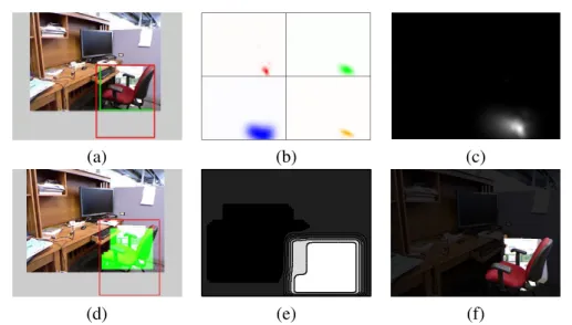
Although many context-aware object detection methods have been proposed [219, 201, 127, 16], most existing contextual models focus on 2D spatial relationships between objects on the image plane and fewer works have extended the modeling to 3D scenarios [8, 193]. Modeling context from a 3D perspective has several advantages over its 2D counterpart conceptually. First, spatial relationships have smaller variations and are easier to interpret semantically; in addition, more spatial relationships in physical world can be captured, instead of being limited to relative positions on image plane. In particular, joint modeling of an object class and its 3D context may provide effective constraints on the object’s scope on image plane and lead to a coarse-level object segmentation. See Figure 1.2 for an example.
However, the appearance variability of the context around an object could be large. It is therefore challenging to use context as a cue, because we would need to model the variability in the appearance of all of the objects around an object of interest. One key challenge is to generate proper training data to capture all the appearance variations. In addition, moving from 2D to 3D (i.e., depth-encoded) context adds a dimension to be sampled, thus seems to make the problem more difficult.
In response to the difficulty outlined above, the practicality of our method is based on both the problem setting and the model design. Firstly, we consider indoor scenes where object-context spatial regularities such as supporting and attachment are more restrictive (e.g., many objects are either supported by floor or by tables), and scene regularities such as orthogonality and vanishing points are more common due to features of man-made structures. In addition, our model uses depth maps to guide us in building a cleaner context representation, such as separating nearby co-occuring objects (e.g., tables and chairs, keyboards and mice) against wall and floor structures further away. During inference, our depth-encoded codebook design enables an image region to contribute to each object hypothesis in a different manner based on its depth layer. Intuitively, context region produces less concentrated vote for object locations as the increased distance from objects leads to higher uncertainty.
More specifically, we propose a structured Hough voting method that incorporates depth-dependent context into a codebook based object detection model. We design a multi-layer representation of context by sorting image regions into different layers depending on their distance to the object. Each layer provides support for the object hypotheses with information from different aspects of the scene. Intuitively, image cues from the object provide the most informative estimation of object location. Further, the surrounding environment can provide
(a) (b) (c)
(d) (e) (f)
Figure 1.2: Illustration of the proposed object detector. (a)RGB frame with object bounding box (red) and visible part bounding box (green). (b) Object centroid voting from multiple layers. (c)Combined object centroid voting results. (d) Detector output (red) with visibility pattern prediction (green). (e)Object visibility pattern prediction results. (f)Final
segmenta-tion results.
less concentrated but useful information on object location, particularly when the contribution from the object itself is weaker due to occlusion.
In addition to the depth-encoded context codebook, our model generalizes the traditional Hough voting detection methods in two other ways. Firstly, we define a new object hypothesis space in which both the object’s center and its visibility mask will be predicted. Each image patch will generate a weighted vote to a joint score of the object center and its support mask in the image. Secondly, we view occlusion as special contextual information, which could provide cues for object detection and help with reasoning about visibility of object parts. The overall output of our approach is a simultaneous object detection and coarse segmentation.
Finally, the varying availability of auxiliary information is a specific issue we wanted to address in this work. Although RGBD cameras are gaining popularity rapidly, the majority of image data are color images. Therefore, we would like our object detector to train with RGBD data but to test without depth maps. The training process aims to learn a context-aware object detection model which encodes depth cues and a coarse level of 3D relationships. The learned depth-encoded object and context model is then applied to 2D images. More specifically, we use depth to sort image features into different layers, and learn codebook entries so that they minimize appearance and 3D geometric distribution variations.
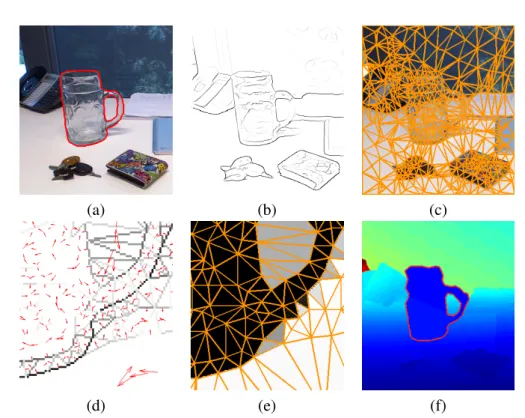
(a) (b) (c)
(d) (e) (f)
Figure 1.3: Illustration of the proposed glass object segmentation system. (a)Intensity image with ground truth foreground mask overlaid.(b)Edge detector output.(c)Triangulation result. (d) Boundary classifier output (magnified). (e) Superpixel classifier output (magnified). (f)
Reconstructed depth with joint inference result overlaid.
1.3
Glass segmentation by joint inference of boundary and region
We aim to localize semi-transparent surfaces by exploring multimodal sensors and incorporat-ing depth information. In particular, we seek to exploit RGBD cameras to fuse the intensity and depth information from a single view point for indoor environments. While recent work with RGBD cameras is mainly for generic object detection [98, 99, 49], here our goal is joint detection, segmentation and depth inference, which can facilitate many interactive tasks such as robotic manipulation. There has been some work exploiting range devices to detect or re-construct semi-transparent objects [209, 84]. Unlike those methods, we rely on a single view RGBD image and combine both intensity and depth cues.
Unlike in Section 1.2 where we take an object-centric view and build an object model that jointly considers the possible object shapes and poses, in this and the following section we focus on the local appearance and depth properties of glass boundary and region. One of the key reasons of taking this local perspective is that glass objects do not have just a few canonical shapes in comparison to some object categories such as cups, bottles, and bowls. See Figure 2.8 for some examples. Arguably, glass objects include subsets of the above object categories: glass cups, glass bottles and glass bowls, etc. While the problem of exploring
the shape and pose constraints for glass objects is interesting, here we focus on capturing the properties of glass objects based on their being made of glass, and the interaction between glass and non-glass regions. Additionally, modeling the specificity of glass material has been proven effective for localizing glass objects in prior literature. For example, some early work focused on detecting special properties of the glass surfaces and their interaction with the opaque environment in images [151, 3, 144] while later ones model the relative features on two sides of a local glass boundary fragment [135, 134] based on a combination of appearance cues. See Section 2.2.4 for a more detailed discussion on the literature.
Taking the local perspective mentioned above, the key idea of our work is to incorpo-rate the spatial context by constructing a Markov Random Field (MRF) [15] on triangularized contour fragments and the corresponding superpixels. Based on spatial neighborhood, we in-corporate constraints between local boundary pairs, superpixel pairs, and boundary-superpixel cliques. More specifically, for each image contour fragment, we estimate if it is likely part of the glass/non-glass boundary, and an orientation for the glass region. For superpixels, we estimate their likelihood being part of the glass region. We add different potentials into our en-ergy function to encourage valid configurations, and penalize incompatible ones. For instance, the orientation for glass regions of two connected glass contour fragments must be the same. For a local clique consisting of a glass contour fragment and two neighboring superpixels, the glass/non-glass labels of both regions must be consistent with the boundary orientation. In addition, a joint inference scheme is designed to predict the glass boundary and region si-multaneously. Our work is the first that jointly optimizes boundary and region properties and constraints for glass object segmentation.
Furthermore, we exploit the refraction and attenuation that will be experienced by an active structured light signal passing through glass objects. This physical process is difficult to model, but it provides a distinctive missing-vs-nonmissing pattern in the depth map. We integrate boundary cues from color with region cues from depth to build a glass boundary and region detector. After we obtained a glass region segmentation with MRF inference described above, we fill in the missing depth values and reconstruct the scene in 3D.
1.4
Depth-aware features and label transfer
The third research problem we discussed in Section 1.1 is the design of depth-aware features and the integration of depth cues into visual inference tasks. In response, we design a number of novel depth-aware features for glass boundary estimation. Most importantly is the distinc-tive missing-vs-nonmissing pattern which we found to be highly effecdistinc-tive for coarsely local-izing glass objects, so we compute the ratio of pixels with missing depth readings in a local image region as a depth feature. Other features include range (depth) histograms and histogram of oriented gradient (HOG) features computed on depth maps. We also explore building a
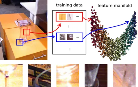
flex-training data ... ... ... ... feature manifold
Figure 1.4: Top: Illustration of feature manifold based glass boundary classification. We use a learned feature manifold to match every boundary fragment in a test scene (shown as image patches) to training set in order to predict its label. Bottom: Large variation on glass
boundaries: patches examples.
ible feature pool which contains both depth and color features. We augment the image cues by sampling features on multiple scales and at multiple locations.
One key reason for the challenging nature of glass object segmentation is the large ap-pearance variations at glass boundaries, as shown in a few examples in Figure 1.4. Training a generic classifier for glass boundaries tends to produce unreliable predictions. Even with RGBD cameras, the missing patterns on depth maps can be noisy, or distorted due to local refractive properties. To address this feature variation issue, we propose an image adaptive ap-proach to predicting glass boundaries. The main idea is to generate boundary proposals based on a nonparametric feature model. Our model is represented by a joint depth and appearance feature manifold, on which each point is the glass boundary feature of an image patch pair. The boundary label of any pair of neighboring patches is predicted by a weighted voting of its nearest neighbors on the feature manifold. The distance metric on the manifold is learned in a supervised manner.
We then integrate the locally adapted glass boundary predictor into a superpixel-based pairwise MRF for glass object segmentation. The MRF labels every superpixel as glass ver-sus non-glass, in which our boundary prediction is used to modulate the smoothing terms in random fields. Our work is the first to explore nonparametric label transfer within the context of glass object segmentation, and exploit a joint depth-appearance manifold for transductive learning.
1.5
Learning from sparsely labeled data
The ground-truth annotation availability issue led us to the development of a boosting-based semi-supervised learning algorithm. Our method adopts a novel data-dependent margin distri-bution learning criterion, which utilizes the intrinsic geometric structure of datasets. One key aspect of our method is that it can seamlessly incorporate unlabeled data by including a graph Laplacian regularizer.
Boosting algorithms have achieved great popularity in a spectrum of computer vision prob-lems due to their good generalization, robust performance, and intrinsic feature selection mech-anism. One key observation related to our work is that the appealing properties of boosting are closely related to themargin distribution(MD) instead of solely the minimum margin [168]. Notably, Shen and Li [182] proposed a totally corrective boosting algorithm, termed MDBoost, to maximize the average margin while minimizing margin variance. The new boosting method achieves competitive performance and faster convergence (i.e., fewer weak learners) on several classification tasks.
Inspired by manifold learning, we propose to improve MDBoost by incorporating a local representation of margin variance, in which only neighboring points on the data manifold con-tribute to the variance computation. Intuitively, the data-dependent margin variance may give a better description of the margin distribution. Due to its resemblance to the Laplacian Eigen-map [10], we refer to this new boosting approach as Laplacian MDBoost. Importantly, our learning criterion can be naturally generalized to a semi-supervised learning scenario. Given both labeled and unlabeled data, we augment the supervised learning criterion with a graph Laplacian-based regularization term, which encourages the classifier outputs on unlabeled data to satisfy the data manifold constraint. This combined learning criterion provides a coherent framework and admits a simple convex quadratic dual formulation such as MDBoost. We em-ploy a column-generation (CG) based optimization procedure to incrementally add informative weak learners, yielding a boosting-like algorithm. The efficacy of the proposed algorithm has been demonstrated in our glass object segmentation experiment, in addition to another video object segmentation task.
1.6
Thesis outline
The next chapter discusses some prior literature that is relevant to the problems addressed in this thesis. It first reviews object detection algorithms, and categorizes them according to two most popular paradigms: the sliding window detector and the Hough transform detector, and their variants and extensions. Next, we discuss work on object detection with RGBD data and context reasoning. The chapter then moves on to object segmentation algorithms, focusing on foreground object segmentation and context modeling with MRFs. After that, we discuss work
on glass object segmentation. Finally, we review work related to the proposed semi-supervised boosting algorithm.
In Chapter 3, we describe a structured Hough voting method for detecting objects with heavy occlusion in indoor environments. First, we extend the Hough hypothesis space to include both object localization, and the object’s visibility pattern. We design a new score function that accumulates votes for object detection and occlusion prediction. In addition, we explore the correlation between objects and their environment, building a depth-encoded object-context model based on RGBD data. Particularly, we design a layered context repre-sentation and allow image patches from both objects and backgrounds to vote for the object hypotheses. We demonstrate that using a data-driven 2.1D representation we can learn visual codebooks with better quality, and obtain more interpretable detection results in terms of the spatial relationship between objects and viewer. We test our algorithm on two challenging RGBD datasets with significant occlusion and intraclass variation, and demonstrate the supe-rior performance of our method.
Chapter 4 addresses the problem of localizing glass objects with a multimodal RGBD camera. Our method integrates the intensity and depth information from a single view point, and builds an MRF that predicts glass boundary and region jointly. Based on the segmentation, we also reconstruct the depth of the scene and fill in the missing depth values. The efficacy of our algorithm is validated on a new RGBD glass dataset of 43 distinct glass objects.
Chapter 5 also addresses the glass object segmentation problem with an RGBD camera. Our approach uses a nonparametric, data-driven label transfer scheme for local glass boundary estimation. A weighted voting scheme based on a joint feature manifold is adopted to inte-grate depth and appearance cues, and we learn a distance metric on the depth-encoded feature manifold. Local boundary evidence is then integrated into an MRF framework for spatially coherent glass object detection and segmentation. The efficacy of our approach is verified on our RGBD dataset where we obtained a clear improvement over the state-of-the-art both in terms of accuracy and speed.
In Chapter 6, we propose a novel data-dependent margin distribution learning criterion for boosting, termed Laplacian MDBoost, which utilizes the intrinsic geometric structure of datasets. One key aspect of our method is that it can seamlessly incorporate unlabeled data by including a graph Laplacian regularizer. We derive a dual formulation of the learning problem that can be efficiently solved by column generation. Experiments on various datasets validate the effectiveness of the new graph Laplacian based learning criterion in both supervised and unsupervised learning settings. We also show that our algorithm outperforms the state-of-the-art semi-supervised learning algorithms on a variety of inductive inference tasks, including glass region classification and real world video segmentation.
Chapter 7 summarizes the main results from this thesis and discusses future research di-rections.
1.7
Major contributions
In this section, we summarize the main differences between our methods and other object detection and segmentation methods, and list the most important results reported in this thesis. • We propose a structured Hough voting model for indoor object detection and occlusion prediction. We extend the original Hough voting based detection model by introducing a joint Hough space of object location and visibility pattern. The structured Hough model can naturally incorporate both the object and its spatial context, which is especially important for cluttered indoor scenes.
• We utilize depth information at the training stage of the structured Hough voting model to build a multilayer object-context model so that a better visual codebook is learned and more detailed object-context relationships can be captured. We use depth information only in the model training stage to learn an appearance model for the surrounding envi-ronment of an object with higher quality, which transfers the depth knowledge for a test scenario which uses color images only.
• We propose a novel joint inference approach to glass object segmentation with RGBD cameras. By setting up an MRF which jointly encodes boundary fragment and super-pixel properties and constraints, we propose a global optimization procedure for glass detection, segmentation and scene reconstruction.
• We propose a glass boundary detection approach by label transfer on joint depth and appearance manifolds. We design novel features for glass object segmentation and a flexible feature pool for improving performance. In addition, our work is the first to explore nonparametric label transfer within the context of glass object segmentation, and exploit a joint depth-appearance manifold for transductive learning.
• We propose a semi-supervised boosting algorithm based on the margin distribution boost-ing. We use the graph Laplacian as an effective means of manifold regularization on both labeled and unlabeled data. The algorithm is totally-corrective and a column generation based optimization technique is used to facilitate minimizing the objective function. The efficacy of this algorithm has been demonstrated on two object segmentation tasks.
Literature Review
Object detection and object segmentation are two popular paradigms for object recognition, which is a key aspect of resolving the gap between low level image features and high level semantic concepts in a scene. There is an abundance of prior literature on both problems. In addition, both problems are based on a classification model for the object/non-object member-ship. In this chapter, we review object detection and segmentation approaches in the literature, with a focus on those that overlap with our research problems discussed in Section 1.1: 1) occlusion and context reasoning, 2) object detection with RGBD data and 3) semi-transparent object detection and segmentation. We also review work on semi-supervised learning that aims at utilizing unlabeled data for classification.
The rest of this chapter is organized as follows. We first discuss popular object detection algorithms in Section 2.1. In particular, we look at methods with occlusion and context rea-soning. Section 2.2 reviews foreground object segmentation algorithms, with a focus on those based on Markov Random Fields (MRFs), a unifying framework for object segmentation and image labeling. In addition, we discuss methods designed to localize semi-transparent objects, a class of objects that are particularly challenging to detect due to their special refractive prop-erties. We then discuss learning a classification model for these systems with partially labeled data in Section 2.3, followed by a summary in Section 2.4.
2.1
Object detection in computer vision
The object detection task is to infer the location of objects belonging to a specific category in an image. In most cases, we are interested in identifying objects from a basic and entry level category[80, 150], which is at a level of abstraction in a taxonomy that carries the most information, possesses the highest category cue validity, and are, thus, the most differentiated from one another [172]. For the horse in Figure 1.1, for example, we will use the entry level categoryhorse instead ofanimalorEquus ferus caballus. Recognizing objects requires dis-criminating them from other objects, while also generalizing over appearance variations within that category. The challenge of this task lies in the delicate contention between specificity and
generality. For example, detectinghorserequires us to differentiate them fromcow,sheepand
person, while being able to detect different subspecies and from various viewpoints.
More specifically, suppose we have an imageI and an object category of interesto. An object is parametrized by a hypothesisx∈ X whereX is the object pose space inI. A basic and common parametrization ofx is a bounding box x= (ax, ay, as, ar), where ax and ay are the image coordinates of the object center, as is a scale, andar is an aspect ratio. Most object detection systems define a scoring function S(o,x) for each valid location x on the image plane, and all hypotheses with a scoreS(o,x)above a certain threshold are claimed as detected objects.
Evaluation of bounding box predictions can be performed by the Jaccard index defined as
J=area(x1∩x2)
area(x1∪x2)
(2.1) where usually a predicted bounding box that has more than50%Intersection-over-Union (IoU) overlap with the ground-truth is considered correct [43].
In the next two sections, we discuss two popular object detection strategies, i.e., sliding window detectors and Hough transform-based detectors. The former takes a top-down, object centric view by examining all possible object locations, while the latter takes a bottom-up, feature centric view by accumulating votes for object locations. However, we note the two strategies are not fundamentally different from each other. The actual difference is more of an algorithmic nature, i.e., how the score is evaluated for all possible object hypotheses [107]. In Section 2.1.3, we continue our discussion by looking at the impact of RGBD camera on object detection with the new challenges it presents. This is followed by discussions on difficult cases for object detection, specifically occlusion reasoning in Section 2.1.4 and context handling in Section 2.1.5.
2.1.1 Sliding window detectors
One of the most popular object detection paradigms is the sliding-window classifier, e.g., [207, 38]. The underlying assumption is the label (e.g., object/non-object) for each bounding box can be obtained independently from labels of other bounding boxes, so the algorithm exhaustively scans through the image with candidate object windows at various locations and scales. This strategy is straightforward, as it evaluates one object candidate at a time and ignores the spatial context that can be more intricate to consider. More importantly, the scan can be naturally viewed as a matching process, so we can define a score that quantifies the match between an object candidate and the object template (e.g., the parameters of the classifier). In its basic form, the scoring function for object detection in this scenario can be written as a linear model:
(a) (b) (c)
Figure 2.1: Visualization of HOG feature space. (a) input image. (b)HOG cells and local gradient orientations. (c)A visualization of HOG features using method in [208].
S(o,x) =βT·Φ(x,I) (2.2) whereΦ(x,I)is a feature function andβis the associated weight vector. The feature function takes the image I and a bounding boxx as input and returns a feature vector that encodes the appearance of the bounding box. To counter the intraclass appearance variation within a specific category, feature functions usually provide some level of invariance to color, shape, deformation, etc. Although in principle it is possible to use raw pixel values from the bounding boxxas the feature vector, more effective features that can achieve a higher level of invari-ance are commonly used, including Haar-like features [207], SIFT descriptors [121], Local Binary Patterns (LBP) [146], and Histograms of Oriented Gradients (HOG) features [38]. See Figure 2.1 for an example of visualizations of the HOG feature space. The weight vector β is usually obtained by discriminative training algorithms such as Support Vector Machines (SVM) [15] or Boosting [207].
Since the advent of deep Convolutional Neural Networks (CNNs) such as AlexNet [94], ZFNet [231] and VGGNet [187], they have been successfully applied to object detection and is now a key component of many state-of-the-art object detection algorithms. Girshick et al. [58] proposed to use a computationally expensive CNN to compute features for a relatively small number of image region proposals. The region proposal step has later been able to share computation with feature extraction [57] and further fully integrated into the CNN as a region proposal network [167]. The most important contribution of a CNN is its ability to extract low dimensional (e.g., 4096-D) but high quality image features, due to the deep structure of the network. Very recently, He et al. [68] proposed residual networks that are significantly deeper than previously used networks. OverFeat [180] is another CNN-based object detection method that uses an efficient sliding window scheme to share computations and apply a CNN densely