www.atmos-chem-phys.net/14/4297/2014/ doi:10.5194/acp-14-4297-2014
© Author(s) 2014. CC Attribution 3.0 License.
Atmospheric
Chemistry
and Physics
CLAAS: the CM SAF cloud property data set using SEVIRI
M. S. Stengel1, A. K. Kniffka1, J. F. M. Meirink2, M. L. Lockhoff1, J. T. Tan1, and R. H. Hollmann1
1Deutscher Wetterdienst (DWD), Offenbach, Germany
2Royal Netherlands Meteorological Institute (KNMI), De Bilt, the Netherlands
Correspondence to: M. Stengel (martin.stengel@dwd.de)
Received: 5 August 2013 – Published in Atmos. Chem. Phys. Discuss.: 11 October 2013 Revised: 13 March 2014 – Accepted: 23 March 2014 – Published: 30 April 2014
Abstract. An 8-year record of satellite-based cloud
prop-erties named CLAAS (CLoud property dAtAset using SE-VIRI) is presented, which was derived within the EUMET-SAT Satellite Application Facility on Climate Monitoring. The data set is based on SEVIRI measurements of the Me-teosat Second Generation satellites, of which the visible and near-infrared channels were intercalibrated with MODIS. Applying two state-of-the-art retrieval schemes ensures high accuracy in cloud detection, cloud vertical placement and mi-crophysical cloud properties. These properties were further processed to provide daily to monthly averaged quantities, mean diurnal cycles and monthly histograms. In particular, the per-month histogram information enhances the insight in spatio-temporal variability of clouds and their properties. Due to the underlying intercalibrated measurement record, the stability of the derived cloud properties is ensured, which is exemplarily demonstrated for three selected cloud vari-ables for the entire SEVIRI disc and a European subregion. All data products and processing levels are introduced and validation results indicated. The sampling uncertainty of the averaged products in CLAAS is minimized due to the high temporal resolution of SEVIRI. This is emphasized by study-ing the impact of reduced temporal samplstudy-ing rates taken at typical overpass times of polar-orbiting instruments. In par-ticular, cloud optical thickness and cloud water path are very sensitive to the sampling rate, which in our study amounted to systematic deviations of over 10 % if only sampled once a day. The CLAAS data set facilitates many cloud related applications at small spatial scales of a few kilometres and short temporal scales of a few hours. Beyond this, the spa-tiotemporal characteristics of clouds on diurnal to seasonal, but also on multi-annual scales, can be studied.
1 Introduction
Cloud property data sets derived from satellite measurements enable global to regional analysis of the spatial and temporal variability of cloud occurrence and specific cloud properties. Different satellite sensor families and types facilitate differ-ent analyses and applications due to their individual instru-mental characteristics, such as the provided spectral bands or scan modi, or with respect to the time period their measure-ments are available.
One well-established satellite sensor type often used in re-mote sensing of cloud properties is the passive VIS/IR im-ager measuring in selected bands in the visible (VIS), near-infrared (NIR) and near-infrared (IR) part of the electromagnetic spectrum. One example of this type is the Advanced Very High Resolution Radiometer (AVHRR) sensor family, which has been flown on NOAA (National Oceanic and Atmo-spheric Administration) and MetOp (Meteorological Oper-ational Satellite) series of polar-orbiting satellites for more than three decades. Corresponding cloud property data sets are for example the CMSAF cLoud, Albedo and RAdiation data set version 1 (CLARA-A1; Karlsson et al., 2013) and the AVHRR Pathfinder Atmospheres – Extended version 6 (Patmos-X; Heidinger and Pavolonis, 2009; Heidinger et al., 2010).
In the years 2000 and 2002 the space component of pas-sive VIS/IR imager on polar-orbiting satellites has been enriched by the Moderate Resolution Imaging Spectrora-diometer (MODIS) instruments, mounted onboard the polar-orbiting satellites Aqua and Terra, with higher spatial resolu-tion and more spectral bands than precursor instruments (see also Platnick et al. (2003) for MODIS-based cloud proper-ties). The most obvious disadvantage of the orbital properties of polar-orbiting instruments is the low temporal sampling
4298 M. Stengel et al.: The CLAAS data set
rate. A big enhancement in this respect is given by geosta-tionary instruments, which although only measuring parts of the globe, provide observations for all covered regions with high temporal resolution.
Considering the observations of passive VIS/IR sensors in both polar and geostationary orbits, the International Satellite Cloud Climatology Project (ISCCP, Rossow and Schiffer, 1999) combined corre-spondingly derived cloud properties in one data set. This leads to a better spatiotemporal coverage compared to data sets purely based on polar-orbiting sensors. This, however, is at the cost of reduced spectral information due to utilization of the overlapping spectral channels only, which is limited by the older geostationary instruments.
The most advanced, currently existing geostationary pas-sive imager is the Spinning Enhanced Visible and InfraRed Imager (SEVIRI). This instrument has been available since 2003 (its operational phase started in 2004), and is now avail-able on the third of the Meteosat Second Generation satel-lites Meteosat-10, in addition to Meteosat-8 and Meteosat-9. Their continuous operational service has created a growing measurement record of nearly one decade. This record now allows for applications with longer temporal scales, going beyond (very) short-term related applications such as now-casting.
In this article we present the data set CLAAS (CLoud property dAtAset using SEVIRI), which contains cloud properties derived from SEVIRI measurements from Meteosat-8 and Meteosat-9 satellites. This work has been done within the framework of the EUMETSAT (European Organisation for the Exploitation of Meteorological Satel-lites) Satellite Application Facility on Climate Monitoring (CM SAF, Schulz et al., 2009). The intercalibration applied to the visible and near-infrared channels of both SEVIRI instruments creates a solid basis for a homogeneous cloud property data set. The cloud properties are derived by using two state-of-the-art retrieval schemes. These provide cloud detection, the vertical placement of the cloud and in-cloud properties of optical thickness and effective radius as well as therefrom-derived properties such as thermodynamic phase and cloud water path. The data set is completed by data sum-maries for the retrieved cloud variables: the first two mo-ments (on a daily and monthly basis) as well as monthly mean diurnal cycles and histograms. The presented data set with its high spatial and temporal resolution can serve as a mature source for cloud studies in regions covered by the SE-VIRI field of view, thus roughly speaking in Europe, Africa, the Atlantic, South America and the Middle East. Potential application areas for CLAAS data also cover regional climate model evaluation or model process studies on, for example, the life cycle and diurnal to seasonal cycles of clouds.
With this article a reference for the CLAAS data set shall be provided. After an introduction to the topic, the article in-troduces the SEVIRI instrument and the measurement prepa-ration in Sect. 2. In Sect. 3 we describe the cloud properties
considered and summarize the retrieval schemes employed. This is followed by a description of the composition of the data set in Sect. 4 including the aggregation to higher-level products (averages, histograms, mean diurnal cycles). Sec-tion 5 summarizes the evaluaSec-tion exercises carried out and in Sect. 6 application examples are given and discussed. Sec-tion 7 concludes.
2 Satellite data used
2.1 SEVIRI
The SEVIRI instrument (Schmetz et al., 2002) is flown on board the Meteosat Second Generation satellites Meteosat-8, Meteosat-9 and Meteosat-10, with operational data avail-able from January 2004. It is a passive imager covering the VIS to IR spectrum with its 12 spectral bands, of which three channels are located in VIS, one in the NIR, and eight in the IR spectrum, with the following nominal centre wavelengths: 0.64, 0.75 (broadband, high-resolution visible – HRV), 0.81, 1.64, 3.92, 6.25, 7.35, 8.70, 9.66, 10.80, 12.00 and 13.40 (all in µm). SEVIRI scans the Earth’s disc from south to north in approx. 12 min, followed by data processing and transfer, which completes one imaging cycle of 15 min. Not used in this study but carried out for limited time periods and sub-regions of the disc are SEVIRI Rapid Scan Services (RSS) with imaging cycles shorter than 15 min. The SEVIRI ground resolution (footprints) near the sub-satellite point (SSP) can in a first approximation be assumed to be of rectangular shape. The spatial resolution is 1.67 km for the HRV and 4.8 km for all other channels. The pixels are oversampled leading to sampling distances for nadir view of the pixels of 1 km (HRV) and 3 km (all other channels), respectively. Due to the scan principle the shape and size of the footprints is not equal over the disc. The east–west extent of the footprints rapidly increase in zonal direction with distance from SSP; while the same feature is present for the north–south extent of the footprints with increasing meridional distance for the SSP (EUMETSAT, 2010). As an example, this results in a foot-print size of approximately 4 km (east–west extent) by 6 km (north–south extent) over Central Europe. Even though the positions of Meteosat-8, 9 and 10 were similar, they are not exactly identical. After its launch Meteosat-8 was positioned at 3.9◦E and after Meteosat-9 became operational at 0.0◦in April 2008, Meteosat-8 was moved to 9.5◦E. Even though
the SEVIRI data projection in Level 1B data is aligned at 0.0◦ for all satellites, the positions of the individual
satel-lites change SEVIRI’s viewing geometries slightly. This is an important feature to consider for each SEVIRI instrument. One needs to keep in mind that observations in same pixels were performed under slightly different viewing conditions depending on the time period of observations and the satel-lite. Also, the field of view (called the SEVIRI disc hereafter) naturally depends on the satellite position. This means that
2003 2004 2005 2006 2007 2008 2009 2010 2011 2012 Year
8
9
Meteosat Satellite
Fig. 1. Temporal coverage of 8/SEVIRI and
Meteosat-9/SEVIRI measurements as taken in operational service and as used as the basis for the presented CLAAS data set. Gaps in Meteosat-9/SEVIRI measurements are filled with Meteosat-8/SEVIRI data if exceeding one day. Gaps in the Meteosat-8/SEVIRI record remain unfilled.
the area covered by the SEVIRI disc was positioned slightly eastwards when SEVIRI on Meteosat-9 took over the opera-tional service.
For the presented data set the time frame was limited to Meteosat-8 and 9. The covered time period is shown in Fig. 1 together with the operational availability of both instruments and the short term periods for which Meteosat-8 SEVIRI re-placed Meteosat-9 due to its maintenance or short-term fail-ure. Significant gaps with no data only occurred during the operational servicing of Meteosat-8 SEVIRI in August 2005 and January 2006, both periods shorter than 2 days, and September–October 2006, for which a gap of 2 weeks ex-ists. In Fig. 2 the covered area of SEVIRI measurements is shown.
As discussed in Meirink et al. (2013), the operational EU-METSAT calibration of the SEVIRI solar channels deviates from the MODIS instrument on Aqua, which can be consid-ered as one of the best calibrated instruments at present (e.g. Wu et al., 2013). The SEVIRI solar channels were found to be offset by, on average,−8,−6, and+3.5 % for channels 1 (0.6 µm), 2 (0.8 µm), and 3 (1.6 µm), respectively, compared to MODIS-Aqua for the years 2004 to 2009. The temporal trend in these offsets was about 0.5 % per year for channel 1, and smaller for the other channels. The solar channel radi-ances used for generating the CLAAS data set were based on the above average intercalibration results, but the temporal trends were not taken into account, since these had not been properly identified at the time the CLAAS processing started. For the thermal infrared channels the on-board calibration, as provided by EUMETSAT, has been applied.
It is also important to note that recently a new reprocessed SEVIRI radiance data set became available through EUMET-SAT for all SEVIRI data before May 2008. The reprocessed data follow the effective radiance definition, which was al-ready characterizing the radiance data from May 2008 on-wards (more details can be found in EUMETSAT, 2008). Us-ing the reprocessed radiance data also for the first part of the CLAAS data set spanning time period ensures homogeneity at radiance level.
3 Considered cloud properties in CLAAS and their retrievals
With respect to the spectral information available through SEVIRI, the following cloud properties were derived for each individual SEVIRI time slot considered: cloud mask, cloud top pressure (which is also converted into height and temperature), cloud thermodynamic phase, cloud optical thickness and cloud effective radius – the latter two are then used to process the liquid and ice water path (LWP, IWP) for each liquid and ice cloud pixel, respectively.
– Cloud mask (CMa), cloud fractional cover (CFC):
de-tecting clouds, meaning the identification of those pix-els containing clouds, is the basis of nearly all remote sensing applications using the visible to infrared spec-trum of electromagnetic radiation. Binary and prob-abilistic cloud masks exist for passive imagers. In our framework the applied cloud mask produces a bi-nary decision cloudy/clear-sky, of which the cloudy case covers the two levels filled and cloud-contaminated. The subsequently listed cloud proper-ties are processed in all cloudy pixels (cloud-filled and cloud-contaminated) with the exception of fractional low-level clouds, as reported in Sect. 3.1. For higher-level products this binary cloud mask information is translated into cloud fractional coverage by averaging in space and time.
– Cloud-top pressure, height, temperature (CTP, CTH,
CTT): these properties are used to refer to the corre-sponding properties of the uppermost cloud layer in a pixel column. The vertical placement of the cloud is, for example, crucial for any cloud type analysis. An exemplary application of cloud top temperature is the radiative effect of clouds in the energy budget.
– Thermodynamic phase (CPh): for passive imagers,
de-tecting the phase at the cloud top is often limited to two classes: liquid and ice. However, a few schemes also attempt to distinguish a mixed class from those two classes. This is not done in the schemes used for the presented CLAAS data set. This parameter is needed to determine the cloud type for which optical prop-erties shall be retrieved. Cloud phase retrievals give opportunities, e.g. for studying cloud glaciation pro-cesses during the development of clouds using tempo-rally highly resolved observations. On climate scales, this allows for analyses on the effects induced by aerosol and dynamics.
– Cloud optical thickness (COT): the vertically
inte-grated optical thickness at 0.6 µm derived in pixels as-signed to be cloud filled.
– Effective radius: the particle surface-area-weighted
4300 M. Stengel et al.: The CLAAS data set
Fig. 2. Examples of pixel-based CLAAS products for (a) cloud mask (CMa), (b) cloud top pressure (CTP), (c) cloud thermodynamic phase
(CPh), (d) cloud optical thickness (COT), (e) liquid water path (LWP), and (f) ice water path (IWP). For the cloud mask plot, dark grey is cloud filled and light grey cloud contaminated. For cloud phase, light grey stands for liquid clouds and dark grey for ice clouds. While CMa and CTP products are processed at the full SEVIRI field of view, the retrieved optical properties REF and COT (and therefrom derived products CPh, LWP, IWP) are restricted to satellite zenith angles smaller than 72◦. Water surface regions contaminated with sunglint are also omitted. All products are on native SEVIRI projection and resolution and shown for 15 July 2006 at 11:45 UTC.
usually treated as round spheres, while for ice crys-tals various habits are assumed, given the wide range of shapes occurring in nature such as plates, columns, droxtals and aggregates.
– Cloud water path: this variable refers to the vertical
integral of cloud condensate, either for liquid clouds (LWP) or ice clouds (IWP), depending on the retrieved thermodynamic phase at the cloud top.
3.1 MSGv2010
For the detection of clouds and their vertical placement, the MSG NWC software package version v2010 was employed, which was developed within the framework of the EUMET-SAT Satellite Application Facility on Support to Nowcast-ing and Very Short Range ForecastNowcast-ing. The cloud detection procedure is documented in Derrien and Le Gléau (2005) and NWCSAF (2010). In brief, the cloud detection proce-dure is composed of a multi-spectral threshold method dur-ing which multiple threshold tests are sequentially applied. The tests depend on, among other things, the illumination (daytime, twilight, night-time, sunglint) and surface type. Because of the variety of tests, different accuracies can be reached. The output of this procedure is a pixel-based mask with the following levels: non-processed, cloud-free, cloud
contaminated, cloud filled, snow/ice contaminated (cloud-free), and undefined. The option of restoring stationary low and mid-level clouds in twilight conditions by carrying for-ward/backward daylight/night-time detection information in time (Derrien and Le Gléau, 2010) has been enabled in our processing. The MSGv2010 package also infers the cloud type for each cloudy pixel (Derrien and Le Gléau, 2005; NWCSAF, 2010). This information is, among others, used in the vertical placement of clouds. The vertical placement of the clouds is done via a cloud top pressure retrieval which is dependent on the cloud type. For very low, low, mid-level and high thick clouds the simulated 10.8 µm bright-ness temperature is fitted to the measurement by modulat-ing the cloud top pressure includmodulat-ing a special treatment of cases with temperature inversions. For high semi-transparent clouds, the H2O/IRW (InfraRed Window) intercept method
is applied (Schmetz et al., 1993), which, if not successful, is followed by the radiance rationing method (Menzel et al., 1983). If this method leads to cloud top temperatures warmer than the 10.8 µm measurement, the approach as applied for thick clouds is used. For pixels, for which the cloud typ-ing assigns fractional clouds (which are mainly low-level water clouds), no attempt is made to retrieve the cloud top parameters. It needs to be noted that the brightness tem-perature simulations are performed at a coarser resolution
of 16 by 16 SEVIRI pixels. The radiative transfer model used is the Radiative Transfer Model for TOVS (RTTOV: Eyre, 1991; Saunders et al., 1999). Radiative transfer calcu-lations for these scenes are conducted assuming grey body clouds separately at various atmospheric levels in addition to clear-sky conditions. Mandatory atmospheric and surface properties are taken from ERA-Interim reanalysis fields (Dee et al., 2011). The reader is referred to NWCSAF (2010) for more information on the MSGv2010 retrieval package. Fig-ure 2 shows examples of MSGv2010 products, which are dis-cussed in Sect. 4.1.
3.2 CPP
The Cloud Physical Properties (CPP, Roebeling et al., 2006; KNMI, 2012) algorithm uses SEVIRI’s VIS and NIR mea-surements to retrieve cloud optical thickness (COT) and cloud particle effective radius (REF) by applying the clas-sical Nakajima and King (1990) approach. This approach is based on the basic feature that the reflectance at a non-absorbing wavelength is primarily related to COT, while the reflectance at an absorbing wavelength is mainly related to REF. For SEVIRI retrievals the VIS 0.64 µm and the NIR 1.63 µm channels have been used here as non-absorbing and absorbing channels, respectively. CPP is based on look-up tables (LUTs) of top-of-atmosphere reflectances for plane parallel, single-layer, liquid and ice clouds, simulated by the Doubling Adding KNMI (DAK) radiative transfer model (Stammes, 2001). Spherical water droplets and imperfect hexagonal ice crystals (Hess et al., 1998) have been used in these simulations, respectively. Absorption by atmospheric trace gases is taken into account based on MODTRAN sim-ulations (Berk et al., 2000). For cloudy pixels, as determined by the MSGv2010 cloud mask, COT and REF are retrieved by matching the observed reflectance to the LUTs. First the ice cloud LUT is tried. If this leads to a match and if the cloud top temperature is below 265 K, the thermodynamic phase is set to ice. Otherwise, the water cloud LUT is used, and the phase is set to liquid. Because the retrieval of effec-tive radius for thin clouds is inherently very uncertain, the retrieved effective radius is weighed with a climatological value of 8 µm for water clouds and 26 µm for ice clouds, re-spectively. The weight of the climatological value is given by a smooth function increasing from 0 at COT≥8 to 1 at COT = 0. The weighting of effective radius affects typically 70 % of the pixels inside the SEVIRI disc, but has an overall effect of only a few percent on the mean cloud water path, because that is governed by the thicker clouds. Liquid or ice water path is then calculated following Stephens (1978):
LWP/IWP=2/3·ρl/i·REF·COT, (1)
whereρl/iis the density of water and ice, respectively.
Equa-tion (1) assumes a vertically homogeneous distribuEqua-tion of cloud condensate. For the retrieved parameters COT, REF,
LWP and IWP, uncertainty estimates are derived by for-ward propagation of 3 % uncertainty in the VIS and NIR re-flectances. This estimate of 3 % follows from an estimated uncertainty in the MODIS solar bands of 2 % (Wu et al., 2013) with some added uncertainty related to the SEVIRI– MODIS intercalibration. Inputs for CPP are the cloud mask from MSGv2010, surface albedo at the VIS and NIR chan-nels based on MODIS data (Moody et al., 2005), and wa-ter vapour path from the ERA-Inwa-terim data set. Analysis has shown that cloud property retrievals become very uncertain at high solar zenith angles (SZAs) and viewing zenith angles (VZAs). Therefore, no retrievals are performed for SZAs or VZAs larger than 72◦. In addition, because sunglint com-plicates the retrieval, possibly sunglint-affected pixels over ocean are excluded. The sunglint is identified by the com-puted glint angle. Areas with glint angles below 25° were assigned sunglint. CPP has been extensively validated using ground-based observations (e.g. Wolters et al., 2008; Roe-beling et al., 2008). Detailed information on the CPP version used to generate the CLAAS data set can be found in KNMI (2012).
As for MSGv2010 products, examples of CPP products are shown in Fig. 2 and discussed in Sect. 4.1.
4 Composition of the data set
The CLAAS data set is composed of cloud products at dif-ferent processing levels from pixel-based data to daily and monthly summaries, such as daily and monthly averages and standard deviations as well as monthly mean diurnal cycles and monthly histograms. An overview on the portfolio is given in Table 1. The corresponding valid ranges are given in Table 2. The characteristics of the products of these pro-cessing levels are described in the following. It needs to be noted that the spatial coverage of all products of all process-ing levels undergo an eastward shift after the transition of Meteosat-8 to Meteosat-9 due to the differing satellite posi-tions. Information on data access and subsequently derived radiation products can be found at http://dx.doi.org/10.5676/ EUM_SAF_CM/CLAAS/V001.
4.1 Pixel-based products
The spatial characteristics of the pixel-based products are identical to the SEVIRI imaging projection and resolution. Thus, the spatial resolution is, as mentioned in Sect. 2.1, ap-prox. 3 by 3 km near the sub-satellite point, with the area gen-erally increasing with satellite zenith angle. The shape, how-ever, is dependent on the exact position of each pixel (e.g. 4 by 6 km over Central Europe).
Figure 2 shows examples of cloud mask and cloud top pressure retrievals for the complete SEVIRI disc for one time step. The cloud mask in panel a indicates the clear-sky pixels and pixels which contain clouds, although the latter
4302 M. Stengel et al.: The CLAAS data set
Table 1. Overview of CLAAS cloud products (indicated by “y”) per cloud variable and processing level: pixel-based products on hourly
resolution, daily mean (DM), monthly mean (MM), monthly mean diurnal cycle (MMDC) and monthly histograms (MH stands for 1-D histograms, JCH for two-dim. COT/CTP histograms). Subscript “dn” denotes that an additional separation for day and night-time values is available and “li” denotes an additional separation for liquid and ice clouds.
Pixel based DM and MM MMDC MH 2dim-H
CFC y ydn y – – CTP, CTH, CTT y y y y – CPh y y y – – COT yli yli yli yli – LWP y y y y – IWP y y y y – JCH – – – – yli Spat. resolution 3–5 km 0.05◦ 0.25◦ 0.05◦ 0.25◦ Projection SEVIRI lat/long lat/long lat/long lat/long
Table 2. Occurring ranges of CLAAS cloud products per cloud
vari-able and processing level: pixel-based products, daily mean (DM), monthly mean (MM), monthly mean diurnal cycle (MMDC). Pixel-based cloud mask values are 0: non-processed; 1: cloud free; 2: cloud contaminated; 3: cloud filled; 4: snow/ice contaminated; 5: undefined (NWCSAF, 2010). Pixel-based cloud phase values are 0: clear-sky; 1: liquid cloud; 2: ice cloud. The ranges given for the averaged products (DM/MM/MMDC) are as technically specified in NetCDF files; the actual geophysical values used in the averag-ing are in the range as given for pixel-based products. Binary data of pixel-based cloud mask and cloud phase are converted to cloud fraction and liquid cloud fraction in the averaged products.
Pixel based DM/MM/MMDC CMa/CFC [0,1,2,3,4,5] [0–100 %] CTP [50–1000 hPa] [0–1100 hPa] CTH [200–18 600 m] [0–20000 m] CTT [150–340 K] [0–400 K] CPh [0,1,2] [0–100 %] COT [0–256] [0–100] LWP [0–4096 g m−2] [0–10 000 g m−2] IWP [0–6554 g m−2] [0–10 000 g m−2]
are actually separated into two classes: cloudy and cloud-contaminated. In panel b the cloud top pressure is shown, which is derived for pixels characterized as cloudy. In this plot typical cloud regimes can be seen, such as convective systems with low CTP in the Inter-Tropical Convergence Zone (ITCZ) and low stratocumulus fields off the coast of Southwest Africa. In panels c–f examples of CPP results for cloud thermodynamic phase, cloud optical thickness, and liquid and ice water path are shown. In comparison to the MSGv2010 products, the restriction to a smaller area (zenith angle restriction) is visible. Another limitation is the restric-tion to cloudy pixels being either a liquid or ice. Follow-ing this, either liquid or ice water path is retrieved for each cloudy pixel. For the pixel-based products of COT, LWP and IWP uncertainty estimates are provided. These estimates
were not taken into account for the generation of higher-level products in the current data set edition.
4.2 Daily and monthly means
For higher-level products, a reprojection onto a latitude– longitude grid has been performed. This grid spans−90 to 90◦in the latitude and longitude directions with a grid box size of 0.05◦for the averaged products. The (linear)
averag-ing was done on native SEVIRI projection and resolution, which ensures similar observation numbers, followed by a nearest-neighbour reprojection onto the latitude–longitude grid. For CTP an alternative averaging in log space is done additionally to the linear averaging. The logarithmic averag-ing approach might be considered for other variables (e.g. COT) as well in future data set releases. For this release COT was averaged linearly to be consistent with the averaging of LWP and IWP. In addition to the all-over daily and monthly means, containing all 24 hourly slots, CFC is also determined separately for daytime and night-time conditions. It is im-portant to note that the binary cloud mask values of 0 and 1 are averaged to result in mean cloud fraction. In this averag-ing procedure, the value of 1 is assigned to the cloud mask class “cloud-contaminated”, which might lead to some over-estimation in the averaged products. The pixel-based cloud thermodynamic phase is used to generate daily and monthly mean liquid cloud fraction, which is relative to the number of detected cloudy cases in each grid box in the given time frame. Cloud optical thickness averages are separated into statistics for liquid and ice clouds, which are given addition-ally to the all-cloud properties.
It is also important to note that the averages of all cloud properties, except cloud fraction, are in-cloud means. Thus generating all-sky, or grid-mean values, for example for model evaluation, requires the incorporation of the cloud fraction, and possibly also the liquid cloud fraction. For COT, LWP and IWP products in particular, the daytime cloud frac-tion should be used in this respect.
Fig. 3. Examples of monthly averaged CLAAS products for (a) cloud fraction (CFC), (b) cloud top pressure (CTP), (c) liquid cloud fraction
(CPh), (d) cloud optical thickness (COT), (e) liquid water path (LWP) and (f) ice water path (IWP). As for the pixel-based products, the optical properties REF and COT (and therefrom derived products CPh, LWP and IWP) are restricted to satellite zenith angles smaller than 72◦. All averaged products stand for in-cloud averages. Together with the histograms the averaged products are defined on a latitude–longitude grid with a grid box size of 0.05◦. All data are for July 2010.
Figure 3 shows monthly averages of cloud fraction, cloud top pressure, liquid cloud fraction, optical thickness, and liq-uid and ice water path.
4.3 Monthly mean diurnal cycle
Similar to the nominal daily and monthly averaged quanti-ties, a monthly mean diurnal cycle for each cloud property is calculated for each grid cell, which for this product has a width of 0.25◦latitude/longitude. Thus, it is of lower spa-tial resolution than the other cloud products. To compose this product, monthly means are determined for each of the 24 hourly time slots, separately. For COT the diurnal cycle is determined separately for liquid and ice clouds. It needs to be noted that, even though the diurnal cycle data spans 24 h, cloud products CPh, COT, LWP and IWP are for each grid box only available for daylight conditions.
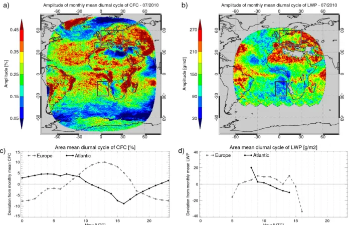
Figure 4 provides an exemplary case study for CFC and LWP for July 2010, showing maps of the amplitude (maxi-mum minus mini(maxi-mum). For this case certain clusters can be found. Highest CFC amplitudes in this month are found for near-coast land regions in South America and Africa in the southern part of the Tropics. The stratocumulus region also exhibits a strong amplitude. Lowest amplitudes are found for ocean regions of the northern and southern mid-latitudes and parts of the Sahara desert. Also shown in Fig. 4 are the rep-resentative diurnal cycles for two selected regions (panels
c and d). The CFC for the central European region shows a characteristic feature with a strong diurnal cycle with max-imum around 13:00 UTC (14:00 LT) and minmax-imum around midnight. The diurnal cycle for the stratocumulus regions also exhibits a characteristic feature for this region: decreas-ing cloud fraction durdecreas-ing daytime with a minimum in the afternoon. Maximum CFC in this regions lies in the early morning.
The same figure also gives the equivalent visualization for LWP. As seen on the map, the available spatial cover-age is reduced. Also, the avercover-age diurnal cycle shown for the two selected regions indicates the missing data for non-daylight conditions. Shorter non-daylight conditions in the se-lected stratocumulus in this month also further limit the tem-poral sampling. It can be seen that the mean LWP for this region shows a general decrease during the day between 08:00 and 14:00 UTC. While this is also indicated in the European region after 09:00 UTC, it seems less pronounced. Also, before 08:00 UTC a strong increase is found, while af-ter 14:00 UTC a very strong decrease is found. While the curve for the stratocumulus region reflects a well-known feature, the shown European cycle needs to be considered with care. The features seen in the morning and evening in this region might partly be caused by retrieval artefacts, which are mainly due to deviations from the plane paral-lel assumption. It needs to be noted that these examples are
4304 M. Stengel et al.: The CLAAS data set
Discussion
P
ap
er
|
Dis
cussion
P
ap
er
|
Discussion
P
ap
e
r
|
Discussion
P
ap
er
|
Fig. 4.
Exemplary maps of monthly mean diurnal cycle of cloud fraction (CFC, panel
(a)
) and
liquid water path (LWP, panel
(b)
, this data was smoothed over 3 neighbouring pixels to better
visualize large scale features). Shown are the respective amplitude (maximum minus minimum)
for each grid box. In the bottom panels, the average values as function of the time of day for
selected regions are shown. The locations of the regions are indicated in the maps. LWP mean
values for selected regions exist only during daylight conditions and are only shown for hours
for which the entire regions were under daylight conditions. All data is for July 2010.
35
Fig. 4. Exemplary maps of monthly mean diurnal cycle of cloud fraction (CFC, (a)) and liquid water path (LWP, (b), these data were smoothed
over three neighbouring pixels to better visualize large-scale features). Shown are the respective amplitude (maximum minus minimum) for each grid box. In the bottom panels, the average values as function of the time of day for selected regions are shown. The locations of the regions are indicated in the maps. LWP mean values for selected regions exist only during daylight conditions and are only shown for hours for which the entire regions were under daylight conditions. All data are for July 2010.
only snapshots to demonstrate the data. They do not reflect the month to month variability that can be expected due to changing weather regimes, in particular for the European re-gion.
4.4 Monthly histograms
To further provide a better representation of the monthly vari-ability of clouds and their properties, histogram information was composed. Here, all inferred cloud data are collected within a spatial grid box and the number of occurrences is aggregated in specific cloud property bins. For each consid-ered cloud property the binning is defined to span the natural variability but with a limited number of bins which reduces the file size. In the case of cloud top pressure the retrieval resolution is also considered. This process resulted in the bin definitions for CTP, COT, LWP and IWP as given in Table 3. The bin definitions for CTP and COT include the ISCCP classifications (Rossow and Schiffer, 1999), but with addi-tional subdivisions. COT histograms are addiaddi-tionally layered for liquid and ice cloud statistics.
In addition to the 1-D histograms, the combinations of CTP and COT were collected and are summarized in 2-D histograms (joint cloud property histograms, JCH). Here, the bin definition for CTP and COT is identical to the 1-D his-tograms, see above. All histograms which include COT, LWP or IWP are limited to daytime data only.
Figure 5 gives an example for the 1-D COT histograms for July 2010, aggregated over the full disc and over two selected subregions – central Europe and a maritime stratocumulus region. Also shown are maps of the relative number of cloud occurrences within two COT ranges (0 to 3.6 and 23 to 100), which were aggregated over the counts of the enclosed bins of the histogram.
Figure 6 gives examples for JCH. Shown are the relative histogram values aggregated over the full disc (panel a). Also shown are the spatial distribution of the relative occurrence of panel b cirrus clouds (CTP above 440 hPa and COT be-tween 0 and 3.6 optical thickness) and panel c stratocumulus clouds (CTP below 680 hPa and COT between 3.6 and 23 op-tical thickness). The classification for these two cloud types are taken from Rossow and Schiffer (1999). As mentioned
P
ap
er
|
Dis
cussion
P
ap
er
|
Discussion
P
ap
e
r
|
Discussion
P
ap
er
|
Fig. 5.
Top panels show maps of relative occurrence of clouds with cloud optical thickness
(COT) between 0 and 3.6
(a)
and between 23 and 100
(b)
. The values were normalized with
the total number of clouds in each grid box. Panel
(c)
reports the histogram of COT aggregated
over a Central European region and panel
(d)
the equivalent for the maritime stratocumulus off
the coast of Angola. Also shown are corresponding cumulative histograms (red). The regions
are indicated in panel
(a)
. All data is for July 2010.
36
Fig. 5. Top panels show maps of relative occurrence of clouds with cloud optical thickness (COT) between 0 and 3.6 (a) and between 23 and
100 (b). The values were normalized with the total number of clouds in each grid box. Panel (c) reports the histogram of COT aggregated over a central European region and (d) the equivalent for the maritime stratocumulus off the coast of Angola. Also shown are corresponding cumulative histograms (red). The regions are indicated in panel (a). All data are for July 2010.
Table 3. Bin borders of CLAAS histograms of cloud top pressure (CTP), cloud optical thickness (COT), liquid water path (LWP), ice water
path (IWP) and joint cloud property histogram (JCH).
CTP [hPa] 1, 90, 180, 245, 310, 375, 440, 500, 560, 620, 680, 740, 800, 875, 950, 1100 COT 0, 0.3, 0.6, 1.3, 2.2, 3.6, 5.8, 9.4, 15, 23, 41, 60, 80, 100
LWP [g m−2] 0, 5, 10, 20, 35, 50, 75, 100, 150, 200, 300, 500, 1000, 2000,>2000 IWP [g m−2] 0, 5, 10, 20, 35, 50, 75, 100, 150, 200, 300, 500, 1000, 2000,>2000
JCH See COT and CTP bins
above, these data are also collected only under daylight con-ditions and for satellite zenith angles lower than 72◦.
5 Evaluation
The CLAAS products of different processing levels have been validated comprehensively against reference observa-tions from ground-based staobserva-tions (SYNOP, lidar–radar obser-vations) as well as space-borne instruments, such as Cloud-Sat, CALIPSO, AMSR-E. In addition, comparisons have been carried out against the retrieved cloud properties of sim-ilar, passive imager instruments (e.g. MODIS). The
evalua-tion results are detailed in Kniffka et al. (2013a) and summa-rized in the following.
Cloud mask evaluation statistics against CALIPSO and CloudSat reflect the high quality of SEVIRI cloud detec-tion with probabilities of detecdetec-tion around 90 %, while false alarm rates are low at 20 to 28 %. The detection efficiency however significantly depends on the optical thickness of the clouds considered, with detection efficiencies significantly decreasing with decreasing optical thickness below 1.
The accuracy of cloud top retrievals such as the cloud top height and thermodynamic phase was validated using CloudSat and CALIPSO as reference. In short, CLAAS SEVIRI-based CTH retrieval has on average a bias of−1 km
4306 M. Stengel et al.: The CLAAS data set
Discussion
P
ap
er
|
Dis
cussion
P
ap
er
|
Discussion
P
ap
e
r
|
Discussion
P
ap
er
|
Fig. 6. (a)
: Joint Cloud property Histogram (JCH) when aggregated over the covered disk (as
shown in panels
(b)
and
(c)
). The values have been normalized with the total number of cloud
occurrences.
(b)
: Relative number of occurrences of cirrus clouds (as defined in Rossow and
Schiffer, 1999) with CTP between above 440
hPa
, and COT between 0 and 3.6.
(c)
: Relative
number of occurrences of stratocumulus clouds with CTP below 680
hPa
, and COT between 3.6
and 23. All data is for July 2010. Grey shaded areas mark regions without cloud observation in
this month.
37
Fig. 6. (a) Joint cloud property histogram (JCH) when aggregated over the covered disc (as shown in panels (b) and (c)). The values have
been normalized with the total number of cloud occurrences. (b) Relative number of occurrences of cirrus clouds (as defined in Rossow and Schiffer, 1999) with cloud top above 440 hPa, and COT between 0 and 3.6. (c) Relative number of occurrences of stratocumulus clouds with cloud top below 680 hPa, and COT between 3.6 and 23. All data are for July 2010. Grey shaded areas mark regions without cloud observation in this month.
considering all clouds. If the sensor sensitivity is considered and the reference CALIPSO height is taken from that cloud level for which the level to cloud layer COT exceeds 0.3, the bias is reduced to−0.6 km. Standard deviations are around 2 km for the filtered subset.
The evaluation of the thermodynamic phase against CALIPSO estimated the probability of detection of ice clouds to be 0.55, while the POD for liquid clouds was sig-nificantly higher at 0.82; which indicates a liquid bias of the phase retrieval. Here however, no COT threshold was ap-plied; and it is assumed that the agreement with CALIPSO would be even better had such a threshold been applied to CALIPSO COT profiles, as was shown for CPP phase re-trievals on AVHRR in Stengel et al. (2013). That study also confirms that CPP retrievals of cloud top thermodynamic
phase are biased towards the liquid phase, in particular for very high, semi-transparent clouds.
COT, LWP and IWP were also compared against MODIS at the pixel level. Results show a good agreement between the two products with standard deviation of 6.2 (bias: 1.8) for optical thickness, 44.9 g m−2(bias:−0.1 g m−2) for liquid water path and 99.2 g m−2 (bias:−6.7 g m−2) for ice water path.
The results discussed in this section are summarized in Ta-ble 4. As mentioned above, the reader is referred to Kniffka et al. (2013a) for all details and aspects of the validations performed.
It needs to be noted that the accuracy of the derived cloud properties show a dependence on satellite–solar geometries. This is most significant for COT and REF (to a smaller
Cloud fraction anomaly 2004 2006 2008 2010 2012 -20 -10 0 10 20 [%] a)
Liquid cloud fraction anomaly
2004 2006 2008 2010 2012 -20 -10 0 10 20 [%] b)
Cloud top pressure anomaly
2004 2006 2008 2010 2012 -40 -20 0 20 40 [%] c)
Fig. 7. Time series of CLAAS relative monthly mean anomaly of cloud fraction (a), liquid cloud fraction (b) and cloud top pressure (c),
averaged over all valid retrievals within the SEVIRI disc (solid lines) and for Europe (dashed lines).
extent) as well as properties derived therefrom. The uncer-tainties here increase with increasing solar zenith angles.
Another problem, which is caused by the satellite view-ing conditions, is the overestimation of cloudiness for large satellite zenith angles due to the slant view. This can lead to increasing systematic errors in higher-level products (e.g. monthly means) in this cloud property with increasing zenith angle (increasing distance from the sub-satellite point). Com-parisons against SYNOP observations show in this respect an overestimation of 10 % on averages for a VZA greater than 70◦, which is the case for example for northern Europe. On the other hand, for a small VZA the viewing conditions of SEVIRI might actually provide a more accurate measure for the cloud fraction than that of the human observer due to its slant observation condition. Averaged over all SYNOP sta-tions within SEVIRI’s disc the cloud fraction bias is slightly positive at about 3 %. Moreover, larger satellite zenith angles introduce a representativeness uncertainty for specific pixels, which on average however should not have a significant sys-tematic effect.
Also investigated was the stability of the data set, which is indicated in Fig. 7. Shown are cloud fraction, liquid cloud fraction and cloud top pressure, all averaged over all pixels within the SEVIRI disc with valid retrievals. This was per-formed for all months and plotted as monthly anomaly from the mean. Also shown are the anomalies for central Europe. All three parameters exhibit a seasonal cycle, whose ampli-tudes are similar for each year.
In general the plots suggest that the presented SEVIRI data are fairly stable in time. No significant trend or jump can be seen, despite the transition from Meteosat-8 to Meteosat-9 in 2007 and temporarily back and forth for some Meteosat-9 data gaps afterwards.
6 Exemplary applications of the data set
In this section we want to highlight the applicability of CLAAS cloud properties, which however will only be of in-dicative character; more detailed follow-on studies are en-couraged for in-depth investigations. One of the strengths of SEVIRI, as mentioned above, is the high frequency of mea-surement sampling for regions covered by its field of view. This enables the observation of spatiotemporally small-scale features, which are present for nearly all clouds and almost all the time, such as the diurnal cycle.
The composition of histograms of cloud properties on a short timescale is made feasible by the high temporal sam-pling of SEVIRI. Such histograms, as for example given in Fig. 5, provide an advanced way to reflect the frequency of the occurrences of the cloud properties. From panel a in this figure it becomes clear that for many regions clouds with COT lower than or equal to 3.6 dominate, in particular over the Atlantic (except stratocumulus regions), Indian Ocean, the Mediterranean and some spots over South America. The relative occurrence of such clouds sometimes amounts to 90 % in these regions. In the month featured in Fig. 5 (July
4308 M. Stengel et al.: The CLAAS data set
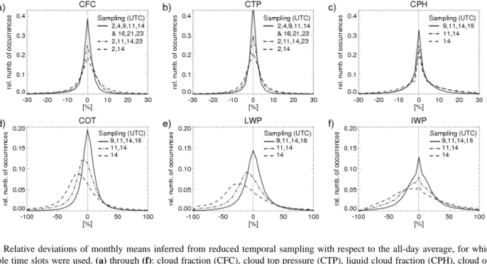
Fig. 8. Relative deviations of monthly means inferred from reduced temporal sampling with respect to the all-day average, for which all
available time slots were used. (a) through (f): cloud fraction (CFC), cloud top pressure (CTP), liquid cloud fraction (CPH), cloud optical thickness (COT), liquid and ice water path (LWP and IWP). For CFC and CTP the monthly means were created from two (02:00, 14:00 UTC), four (02:00, 11:00, 14:00, 23:00 UTC) and eight (02:00, 04:00, 09:00, 11:00, 14:00, 16:00, 21:00, 23:00 UTC) samples a day, while for CPH, COT, LWP and IWP the monthly means were created from one (14:00 UTC), two (11:00, 14:00 UTC) and four (09:00, 11:00, 14:00, 16:00 UTC) samples a day. The data shown are for July 2011 and regions between−20◦and 20◦longitude and with satellite zenith angles lower than 72◦. Note the different scaling of the axes for CFC, CTP and CPH compared to COT, LWP and IWP.
2010), clouds with high COT seem to have made a signifi-cant contribution for European and central African land, the ITCZ, the mid-latitudes over the Atlantic Ocean and south-west South America. For the latter regions, it is most pro-nounced with values up to 20 %. Also very distinct is the difference in histogram skewness between the two selected regions. For Central Europe we find a clear positive skew-ness with a peak around three optical thickskew-nesses. This is in contrast to the stratocumulus region for which the skewness is negative with a peak around 10 optical thicknesses. A more detailed investigation of LWP frequency distribution is doc-umented in Kniffka et al. (2013b).
This investigation highlights on an exemplary basis that the spatiotemporal variability of cloud variables often devi-ates from a Gaussian distribution, which motivdevi-ates the col-lection and provision of histogram information in addition to the mean and standard deviations.
Combining the temporal occurrence of COT and CTP fa-cilitates a cloud type analysis along the lines of the ISCCP (Rossow and Schiffer, 1999). The CLAAS JCH as intro-duced in Sect. 4.4 provides this valuable information on high spatial resolution as well as high resolution in COT and CTP space. In Fig. 6 the aggregation of this fine-resolved infor-mation for two of the classical nine ISCCP cloud classes is shown: (1) cirrus clouds with COT between 0 and 3.6, and CTP above 440 hPa, and stratocumulus clouds with COT be-tween 3.6 and 23, and CTP below 680 hPa (see also panel
a). The data are shown as spatial maps of their relative oc-currence with respect to the total number of clouds detected in each grid box. In the considered month, cirrus clouds, as defined above, have a high relative occurrence in the tropical Atlantic and Indian oceans, in addition to some land regions in South America, middle and northern Africa, as well as eastern Europe and the Iberian Peninsula. In contrast to this, stratocumulus clouds have well defined regions of occur-rences, i.e. in the subsidence regions of the Atlantic Ocean. In addition, some coastal areas, in particular Africa and east-ern South America show similar frequent occurrences of this cloud type. In this context it is very important to notice that with passive imager instruments, such as SEVIRI, usually only the uppermost cloud layer can be identified, thus the occurrences of clouds underneath are not reflected in corre-sponding cloud property statistics. The joint histograms can also be used to characterize certain weather states, as re-ported in Rossow et al. (2005) and Oreopoulos and Rossow (2011).
In the following, the strengths of SEVIRI high temporal resolution shall be highlighted. Figure 8 shows the devia-tions found if cloud properties are only sampled with re-duced temporal resolution. For this the monthly mean values based on temporal sampling of one (14:00 UTC), two (11:00, 14:00 UTC) and four (09:00, 11:00, 14:00, 16:00 UTC) times per day per grid box were subtracted from the nominal monthly mean; the curves show the histogram of relative
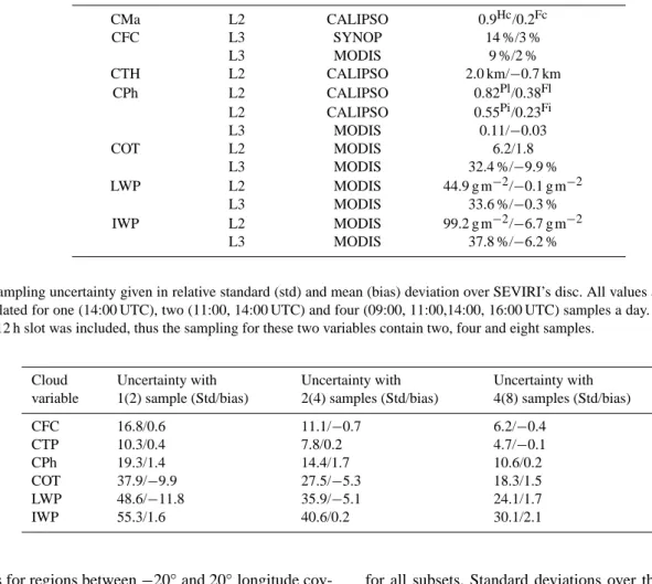
Table 4. Summary of evaluation scores for CLAAS products as there are given in Kniffka et al. (2013a). Processing level L2 stands for
pixel-based products, while L3 refers to monthly averages. The values of standard deviations and biases are reported. Subscripts Hc and Fc refer to hit rate and false alarm for cloud detection. Similarly, Pl, Pi are the probabilities of detection for liquid and ice clouds, while Fl, Fi are corresponding false alarm rates. L2 comparison results for COT, LWP and IWP against MODIS were, in contrast to Kniffka et al. (2013a), extended to cover one month of collocations.
Cloud variable Processing level Evaluation source Evaluation scores (Std/bias)
CMa L2 CALIPSO 0.9Hc/0.2Fc CFC L3 SYNOP 14 %/3 % L3 MODIS 9 %/2 % CTH L2 CALIPSO 2.0 km/−0.7 km CPh L2 CALIPSO 0.82Pl/0.38Fl L2 CALIPSO 0.55Pi/0.23Fi L3 MODIS 0.11/−0.03 COT L2 MODIS 6.2/1.8 L3 MODIS 32.4 %/−9.9 % LWP L2 MODIS 44.9 g m−2/−0.1 g m−2 L3 MODIS 33.6 %/−0.3 % IWP L2 MODIS 99.2 g m−2/−6.7 g m−2 L3 MODIS 37.8 %/−6.2 %
Table 5. Sampling uncertainty given in relative standard (std) and mean (bias) deviation over SEVIRI’s disc. All values are given in % and
were calculated for one (14:00 UTC), two (11:00, 14:00 UTC) and four (09:00, 11:00,14:00, 16:00 UTC) samples a day. For CFC and CTP also the+12 h slot was included, thus the sampling for these two variables contain two, four and eight samples.
Cloud variable Uncertainty with 1(2) sample (Std/bias) Uncertainty with 2(4) samples (Std/bias) Uncertainty with 4(8) samples (Std/bias) CFC 16.8/0.6 11.1/−0.7 6.2/−0.4 CTP 10.3/0.4 7.8/0.2 4.7/−0.1 CPh 19.3/1.4 14.4/1.7 10.6/0.2 COT 37.9/−9.9 27.5/−5.3 18.3/1.5 LWP 48.6/−11.8 35.9/−5.1 24.1/1.7 IWP 55.3/1.6 40.6/0.2 30.1/2.1
deviations for regions between−20◦and 20◦longitude cov-ered by the SEVIRI disc. Since retrievals of CFC and CTP are also possible during night-time, the constructed monthly means are based on two (02:00, 14:00 UTC), four (02:00, 11:00, 14:00, 23:00 UTC) and eight (02:00, 04:00, 09:00, 11:00, 14:00, 16:00, 21:00, 23:00 UTC) samples a day per grid box. The time slots at 11:00 and 14:00 UTC in these considerations were chosen with respect to the local equator crossing times of MODIS-Terra and AVHRR/NOAA-17 as well as MODIS-Aqua and AVHRR/NOAA-18, respectively. For this example the change in local time over the consid-ered regions is neglected. The other two time slots 09:00 and 16:00 UTC could be seen as additional early morning and late afternoon orbits. Table 5 reports standard and mean de-viations over the relative differences. A similar investigation, for cloudiness only, is given in Foster and Heidinger (2013). While a decreasing temporal sampling naturally leads to increasing deviation on average (seen for all cloud variables), for CFC, CTP and CPh very narrow distributions are found
for all subsets. Standard deviations over the relative devia-tions to the nominal monthly means range for CFC and CTP from 10 to 17 % for two daily samples and decrease to 4 to 6 % when using eight samples. Biases are relative small with values always below 0.7. In contrast, panels d–f reveal that the sampling error is much more pronounced for COT, LWP and IWP. Standard deviations for these three variables range from 37 to 55 % when only using one sample a day (also in-dicated by the broad distributions in Fig. 8), which is more pronounced for LWP and IWP than for COT. Partly strong negative biases are found. The values decrease to 18 to 30 % when four samples are used. This effect is assumed to be more pronounced for cloud variables which either are very variable in time in general and/or variables which are char-acterized by a significant diurnal cycle, as is, for example, indicated in Kniffka et al. (2013b) for LWP.
The benefit of this exercise is twofold. It firstly indi-cates that SEVIRI-based products provide a better estimate of an 24 h mean on daily or monthly basis. Secondly, these
4310 M. Stengel et al.: The CLAAS data set
numbers can be used to quantify the uncertainties that can be expected for polar-orbiting instruments, such as AVHRR and MODIS if used with this aim.
7 Summary and outlook
In this article we present a cloud property data set generated within the EUMETSAT Satellite Application Facility on Cli-mate Monitoring and inferred from measurements of the SE-VIRI instrument.
The data set spans the time period from 2004 to 2011 us-ing SEVIRI measurements onboard the satellites Meteosat-8 and Meteosat-9 satellites. Visible and near-infrared mea-surements were intercalibrated with MODIS. Cloud prop-erties considered are cloud mask/fraction, cloud top pres-sure/height/temperature and the microphysical cloud prop-erties effective radius, optical thickness and thermodynamic phase. The microphysical properties are further utilized to re-trieve liquid and ice water path. The properties are inferred on an hourly basis on full SEVIRI spatial resolution, and then further processed on a latitude–longitude grid to com-pose daily and monthly means as well as monthly mean diur-nal cycles and monthly histogram information. Examples of derived cloud properties of different processing levels were shown and discussed. Further, the stability was investigated and demonstrated for cloud fraction, liquid cloud fraction and cloud top pressure, indicating the stability of the prop-erties over the considered period. In particular the transition between the Meteosat-8 and Meteosat-9 satellites does not cause significant jumps in the time series.
The presented data set provides accurate cloud property data within the SEVIRI field of view enabling a large vari-ety of applications. Frequency distributions of cloud optical thickness were discussed on an exemplary basis highlight-ing the capability of SEVIRI to derive mature cloud statis-tics on small spatial and short temporal scales. Also reported was the uncertainty with respect to reduced temporal sam-pling, which firstly is minimized when using SEVIRI, and secondly, can be used to quantify corresponding uncertain-ties for polar-orbiting instruments. While CFC, CTP and CPh show only a small sensitivity, COT, LWP and IWP reveal a strong sensitivity to reduced sampling, which can amount to standard deviations of 55 % when considering relative de-viations from the nominal SEVIRI average when consider-ing all pixels in the SEVIRI disc within one month. Also, the mean relative deviation within the disc can exceed 10 %.
Going beyond the indicated areas, numerous further ap-plications will be possible based on this data set, which are encouraged and envisaged for future studies.
The continued effort of CM SAF towards composing cloud property data sets based on SEVIRI, as the presented CLAAS data set, is planned to result in updates in the near future. This will most likely include the extension of the temporal coverage from 01/2004 to 12/2014 with an increased
tempo-ral resolution of 15 min. Ongoing collection of user feedback will also impact the selection of cloud properties as well as their technical characteristics in the next data set edition.
Acknowledgements. This work has been performed within the framework of the EUMETSAT Satellite Application Facility on Climate Monitoring (CM SAF). The authors would like to thank the EUMETSAT Satellite Application Facility on Support to Nowcasting and Very Short Range Forecasting for the provision of the MSGv2010 algorithm package. Many thanks also go to other CM SAF team members who are not listed as co-authors, but who helped to make this effort succeed.
Edited by: B. Mayer
References
Berk, A., Anderson, G. P., Acharya, P. K., Chetwynd, J. H., Bernstein, L. S., Shettle, E. P., Matthew, M. W., and Adler-Golden, S. M.: MODTRAN4 Version 2 Users Manual, Technical report, Air Force Materiel Command, Air Force Research Lab-oratory, Space Vehicles Directorate, Hanscom AFB, MA 01731, USA, 2000.
Dee, D. P., Uppala, S. M., Simmons, A. J., Berrisford, P., Poli, P., Kobayashi, S., Andrae, U., Balmaseda, M. A., Balsamo, G., Bauer, P., Bechtold, P., Beljaars, A. C. M., van de Berg, L., Bid-lot, J., Bormann, N., Delsol, C., Dragani, R., Fuentes, M., Geer, A. J., Haimberger, L., Healy, S. B., Hersbach, H., Hólm, E. V., Isaksen, L., Kållberg, P., Köhler, M., Matricardi, M., McNally, A. P., Monge-Sanz, B. M., Morcrette, J.-J., Park, B.-K., Peubey, C., de Rosnay, P., Tavolato, C., Thépaut, J.-N., and Vitart, F.: The ERA-Interim reanalysis: configuration and performance of the data assimilation system, Q. J. Roy. Meteor. Soc., 137, 553–597, doi:10.1002/qj.828, 2011.
Derrien, M. and Le Gléau, H.: MSG/SEVIRI cloud mask and type from SAFNWC, Int. J. Remote Sens., 26, 4707–4732, 2005. Derrien, M. and Le Gléau, H.: Improvement of cloud detection
near sunrise and sunset by temporal-differencing and region-growing techniques with real-time SEVIRI, Int. J. Remote Sens., 31, 1765–1780, 2010.
EUMETSAT: On Differences in Effective and Spectral Ra-diance MSG Level 1.5 Image Products, EUMETSAT, Am Kavalleriesand, 31, Darmstadt, Germany, EUM/OPS-MSG/TEN/08/0161 v1, 25 April 2008, 2008.
EUMETSAT: MSG Level 1.5 Image Data Format Description, EUMETSAT, Am Kavalleriesand, 31, Darmstadt, Germany, EUM/MSG/ICD/105, 2010.
Eyre, J.: A fast radiative transfer model for satellite sounding sys-tems, ECMWF Tech. Memo. 186, European Centre for Medium Range Weather Forecasts, Shinfield Park, Reading, Berkshire RG2 9AX, UK, 1991.
Foster, M. J. and Heidinger, A.: PATMOS-x: results from a diurnally corrected 30 yr satellite cloud climatology, J. Climate, 26, 414– 425, 2013.
Heidinger, A. K. and Pavolonis, M. J.: Gazing at cirrus clouds for 25 years through a split window, Part 1: Methodology, J. Appl. Meteorol. Clim., 48, 1100–1116, 2009.
Heidinger, A. K., Straka III, W. C., Molling, C. C., Sullivan, J. T., and Wu, X.: Deriving an inter-sensor consistent calibration for the AVHRR solar reflectance data record, Int. J. Remote Sens., 31, 6493–6517, 2010.
Hess, M., Koelemeijer, R., and Stammes, P.: Scattering matrices of imperfect hexagonal ice crystals, J. Quant. Spectrosc. Rad., 60, 301–308, 1998.
Karlsson, K.-G., Riihelä, A., Müller, R., Meirink, J. F., Sedlar, J., Stengel, M., Lockhoff, M., Trentmann, J., Kaspar, F., Holl-mann, R., and Wolters, E.: CLARA-A1: a cloud, albedo, and ra-diation dataset from 28 yr of global AVHRR data, Atmos. Chem. Phys., 13, 5351–5367, doi:10.5194/acp-13-5351-2013, 2013. Kniffka, A., Lockhoff, M., Stengel, M., and Meirink, J. F.:
Algorithm Theoretical Basis Document for Cloud Phys-ical Products, EUMETSAT Satellite Application Facil-ity on Climate Monitoring, available at: www.cmsaf.eu, SAF/CM/DWDI/VAL/SEV/CLD, Issue 1, Rev. 1, 2013a. Kniffka, A., Stengel, M., Lockhoff, M., Bennartz, R., and
Holl-mann, R.: Characteristics of cloud liquid water path from SE-VIRI on the Meteosat Second Generation 2 satellite for sev-eral cloud types, Atmos. Meas. Tech. Discuss., 6, 8743–8782, doi:10.5194/amtd-6-8743-2013, 2013b.
KNMI: Algorithm Theoretical Basis Document for Cloud Physical Products, EUMETSAT Satellite Application Fa-cility on Climate Monitoring, available at: www.cmsaf.eu, SAF/CM/KNMI/ATBD/SEVIRI/CPP, Issue 1, Rev. 0, 2 Octo-ber 2012, 2012.
Meirink, J. F., Roebeling, R. A., and Stammes, P.: Inter-calibration of polar imager solar channels using SEVIRI, Atmos. Meas. Tech., 6, 2495–2508, doi:10.5194/amt-6-2495-2013, 2013. Menzel, W. P., Smith, W. L., and Stewart , T. R.: Improved Cloud
Motion Wind Vector and Altitude Assignment using VAS, J. Appl. Meteorol. Clim., 22, 377–384, 1983.
Moody, E. G., King, M. D., Platnick, S., Schaaf, C. B., and Gao, F.: Spatially complete global spectral surface albedos: value-added datasets derived from Terra MODIS land products, IEEE T. Geosci. Remote, 43, 144–158, 2005.
Nakajima, T. and King, M. D.: Determination of the optical thick-ness and effective particle radius of clouds from reflected so-lar radiation measurements, Part 1: Theory, J. Atmos. Sci., 47, 1878–1893, 1990.
NWCSAF: Algorithm Theoretical Basis Document for “Cloud Products” (CMa-PGE01 v3.0, CT-PGE02 v2.0 & CTTH-PGE03 v2.1), EUMETSAT Satellite Applica-tion Facility on Nowcasting and Shortrange Forecasting, SAF/NWC/CDOP/MFL/SCI/ATBD/01, Issue 3, Rev. 0, 17 May 2010, 2010.
Oreopoulos, L. and Rossow, W. B.: The cloud radiative ef-fects of International Satellite Cloud Climatology Project weather states, J. Geophys. Res.-Atmos., 116, D12202, doi:10.1029/2010JD015472, 2011.
Platnick, S., King, M. D., Ackerman, S. A., Menzel, W. P., Baum, B. A., Riédi, J. C., and Frey, R. A.: The MODIS cloud products: algorithms and examples from Terra, IEEE T. Geosci. Remote, 41, 459–473, 2003.
Roebeling, R., Feijt, A., and Stammes, P.: Cloud property re-trievals for climate monitoring: implications of differences be-tween Spinning Enhanced Visible and Infrared Imager (SE-VIRI) on METEOSAT-8 and Advanced Very High Resolution
Radiometer (AVHRR) on NOAA-17, J. Geophys. Res.-Atmos., 111, D20210, doi:10.1029/2005JD006990, 2006.
Roebeling, R., Deneke, H., and Feijt, A.: Validation of cloud liquid water path retrievals from SEVIRI using one year of CloudNET observations, J. Appl. Meteorol. Clim., 47, 206–222, 2008. Rossow, W. B. and Schiffer, R. A.: Advances in understanding
clouds from ISCCP, B. Am. Meteorol. Soc., 80, 2261–2287, 1999.
Rossow, W. B., Tselioudis, G., Polak, A., and Jakob, C.: Tropical climate described as a distribution of weather states indicated by distinct mesoscale cloud property mixtures, Geophys. Res. Lett., 32, L21812, doi:10.1029/2005GL024584, 2005.
Saunders, R., Matricardi, M., and Brunel, P.: An improved fast ra-diative transfer model for assimilation of satellite radiance obser-vations, Q. J. Roy. Meteor. Soc., 125, 1407–1425, 1999. Schmetz, J., Holmlund, K., Hoffman, J. and Strauss, B., Mason, B.,
Gaertner, V., Koch, A., and Van De Berg, L.: Operational cloud-motion winds from Meteosat infrared images, Journal of Applied Meteorology, 32, 7, 1206–1225, 1993.
Schmetz, J., Pili, P., Tjemkes, S., Just, D., Kerkmann, J., Rota, S., and Ratier, A.: An introduction to Meteosat second generation (MSG), B. Am. Meteorol. Soc., 83, 977–992, 2002.
Schulz, J., Albert, P., Behr, H.-D., Caprion, D., Deneke, H., Dewitte, S., Dürr, B., Fuchs, P., Gratzki, A., Hechler, P., Hollmann, R., Johnston, S., Karlsson, K.-G., Manninen, T., Müller, R., Reuter, M., Riihelä, A., Roebeling, R., Sel-bach, N., Tetzlaff, A., Thomas, W., Werscheck, M., Wolters, E., and Zelenka, A.: Operational climate monitoring from space: the EUMETSAT Satellite Application Facility on Climate Monitoring (CM-SAF), Atmos. Chem. Phys., 9, 1687–1709, doi:10.5194/acp-9-1687-2009, 2009.
Stammes, P.: Spectral radiance modelling in the UV-visible range, in: IRS 2000: Current Problems in Atmospheric Radiation, edited by: Smith, W. L. and Timofeyev, Y. M., 385–388, A. Deepak, Hampton, VA, 2001.
Stengel, M., S., M., Jerg, M., Karlsson, K.-G., Scheirer, R., Mad-dux, B., Meirink, J., Poulsen, C., Siddans, R., Walther, A., and Hollmann, R.: The Clouds Climate Change Initiative: As-sessment of state-of-the-art cloud property retrieval schemes ap-plied to AVHRR heritage measurements, Remote Sens. Environ., doi:10.1016/j.rse.2013.10.035, in press, 2013.
Stephens, G.: Radiation profiles in extended water clouds, II: Pa-rameterization schemes, J. Atmos. Sci., 35, 2123–2132, 1978. Wolters, E. L. A., Roebeling, R. A., and Feijt, A. J.: Evaluation of
cloud-phase retrieval methods for SEVIRI onboard Meteosat-8 using ground-based lidar and cloud radar data, J. Appl. Meteorol. Clim., 47, 1723–1738, 2008.
Wu, A., Xiong, X., Doelling, D. R., Morstad, D., Angal, A., and Bhatt, R.: Characterization of Terra and Aqua MODIS VIS, NIR, and SWIR spectral bands’ calibration stability, IEEE T. Geosci. Remote, 51, 4330–4338, doi:10.1109/TGRS.2012.2226588, 2013.