F
EDERICO
II
P
H.D. T
HESISI
NS
TATISTICSXXVIII C
YCLEDevelopments in PLS-PM
for the building of a System of
Composite Indicators
Rosanna Cataldo
A thesis submitted in fulfillment of the requirements of the degree of Statistics
in the
for the building of a System of Composite Indicators
Author:
Tutor:
Rosanna Cataldo
M. Gabriella Grassia
University of Naples Federico II
Co-tutor:
Department of Economics and Statistics
N. Carlo Lauro
Via Cintia - Complesso Monte S.Angelo, 26e-mail: [email protected]
Questo lavoro è il risultato di un’esperienza umana e scientifica nata dall’incontro con tante persone. Desidero ringraziare tutti coloro che a vario titolo mi hanno accompagnato in questo percorso e senza le quali non sarebbe stato possibile realiz-zare questo lavoro di tesi.
Devo ringraziare, innanzitutto, la mia Tutor, Prof. M. Gabriella Grassia, per avermi guidato in questo percorso di ricerca con saggi consigli ed avermi seguito costantemente non solo nella realizzazione della tesi di dottorato. Esprimo la mia riconoscenza per aver creduto in me. La sua tenacia mi ha sostenuta anche nei momenti più difficili. La ringrazio per la sua infinita pazienza e per le sue tante ”ramanzine da madre”, le quali mi hanno aiutato a crescere e ad imparare dai miei errori.
E’ mio dovere ringraziare il Prof. N. Carlo Lauro, per essersi sempre dimostrato disponibile ad offrirmi il suo preziosissimo contributo teorico e metodologico du-rante questo lavoro di ricerca, e per i suoi impagabili suggerimenti.
Entrambi hanno rappresentato il ”modello strutturale” di tutto il lavoro, senza il loro apporto, e soprattutto supporto, questo lavoro non avrebbe mai conosciuto la luce del giorno.
Un grazie particolare, inoltre, va a Roberto, che più che una collega si è rivelato essere un’ottimo amico, subendo tutte le mie ansie e inquietudini per la buona riuscita di questo lavoro. Roberto ha costituito il ”modello di misura” della mia ricerca, mi ha seguito costantemente e attentamente nella parte pratica di questo lavoro.
Voglio, infine, ringraziare tutti i colleghi e amici dottorandi con cui ho condiviso lezioni, impegni, preoccupazioni e frustrazioni, oltre a idee e soddisfazioni.
Introduction 1
1 Composite Indicators 7
1.1 Introduction . . . 7
1.2 Definition of Composite Indicators . . . 8
1.3 A quality framework for Composite Indicators . . . 11
1.4 Composite Indicators from different points of view . . . 15
1.5 From Data Driven Composite Indicators to Model Based Com-posite Indicators . . . 18
1.5.1 Theory Based and Data Driven Composite Indicators 19 1.5.2 Model Based Composite Indicators . . . 23
2 Partial Least Squares Path Modeling 26 2.1 Introduction . . . 26
2.2 The PLS path model . . . 27
2.2.1 The Measurement Model . . . 27
2.2.2 The Structural Model . . . 32
2.3 The Partial Least Squares Algorithm . . . 33
2.3.1 The first stage: the Iterative Approximation of LVs . . 33
2.3.2 The second stage: the estimation of the LV scores . . 37
2.3.3 The third stage: the estimation of the path coefficients 37 2.4 Model Validation . . . 39
2.4.1 Assessing the results of reflective measurement models 40 2.4.2 Assessing the results of formative measurement models 43 2.4.3 Assessing the results of structural models . . . 45
2.7 Available software for PLS Path Modeling . . . 51
3 Some developments in PLS - PM for the building of Composite Indicators 54 3.1 Introduction . . . 54
3.2 Non Numerical Models for data measured on different measurement scales . . . 56
3.2.1 Partial Alternating Least Squares Optimal Scaling Path Modeling . . . 56
3.2.2 Non-Metric PLS Path Modeling . . . 58
3.3 The importance of modeling heterogeneity in PLS-PM: Mediator and Moderator Variables . . . 59
3.3.1 Mediator Variables . . . 60
3.3.2 Moderator Variables . . . 62
3.4 An Example: Building an Italian Social Cohesion Composite Indicator (SC-CI) . . . 69
3.4.1 A brief history of Social Cohesion . . . 70
3.4.2 The Social Cohesion Path Modeling Estimation . . . 71
3.4.3 The model . . . 72
3.4.4 Statistical Analysis and Main Results . . . 74
3.4.5 Conclusions for Italian Social Cohesion Composite In-dicator Example . . . 77
3.5 Unobserved Heterogeneity in PLS-PM . . . 78
3.5.1 The PATHMOX Approach . . . 80
3.5.2 The REBUS-PLS Approach . . . 83
3.6 An example: Treating the Heterogeneity of the Legitimacy of Violence Higher-Order CI . . . 86
3.6.1 Measurement Instruments (questionnaires) . . . 87
3.6.2 The model . . . 87
3.6.3 Pre-treatment of data . . . 88
3.6.4 Statistical Analysis and Main Results . . . 89
3.6.8 Conclusions for REBUS-PLS Approach . . . 100
3.7 Conclusions . . . 100
4 Higher-Order Constructs in PLS-PM 102 4.1 Introduction . . . 102
4.2 Estimation of Higher-Order Construct Models . . . 104
4.2.1 Molecular and Molar Higher-Order Construct Models 105 4.2.2 Types of Higher-Order Construct Models . . . 105
4.3 PLS-based Approaches to Estimating Path Models with Higher-Order Constructs . . . 107
4.3.1 The Repeated Indicators Approach . . . 107
4.3.2 The Two Step Approach . . . 110
4.3.3 The Hybrid Approach . . . 113
4.4 A Multidimensional Poverty Composite Indicator based on Higher-Order Constructs . . . 114
4.4.1 A brief history of Poverty Indices . . . 114
4.4.2 The Higher-Order Multidimensional Poverty Com-posite Indicator (MP-CI) . . . 116
4.4.3 The three Higher-Order Constructs Approaches com-pared . . . 118
4.4.4 The Two Step Approach and its results . . . 122
4.4.5 Conclusions for Higher-Order MP-CI . . . 124
4.5 Conclusions . . . 125
5 New methods in PLS Path Modeling for the building a System of Composite Indicators 126 5.1 Introduction . . . 126
5.2 The First Alternative Approach: "The Mixed Two Step Ap-proach" . . . 127
5.2.1 The Mixed Two Step Approach implemented in PLS-PM . . . 128
5.3.1 The PLS Regression method . . . 131
5.3.2 The Regression implemented in Higher-Order PLS-PM . . . 134
5.4 Simulation Study . . . 137
5.4.1 Data Generation . . . 137
5.4.2 Simulation Results: The path coefficients . . . 139
5.4.3 Simulation Results: Bias and efficiency of the param-eters . . . 141
5.4.4 Simulation Results: The LV Prediction Accuracy . . . 142
5.4.5 Simulation Results: Choosing the Best Method . . . . 143
5.5 Application to Real Data: Comparison of Methods . . . 144
5.5.1 Application Results: the Mixed Two Step and the PLS-Component Regression Approaches Performances . . 144
5.5.2 Application Results: Conclusions . . . 149
5.6 Conclusions . . . 150
Conclusions and Future Research 152
2.1 Reflective model in a path diagram . . . 28
2.2 Formative model in a path diagram . . . 30
2.3 Structural model in a path diagram . . . 32
2.4 Redundancy Analysis for Convergent Validity Assessment . 44 3.1 Simple Cause - Effect Relationship and General Mediator Model . . . 60
3.2 A simple model with a moderating effect . . . 62
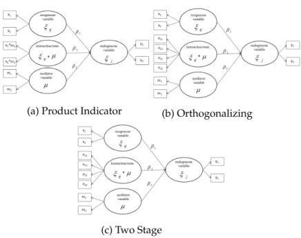
3.3 Approaches for Modeling Interaction . . . 67
3.4 The model for the Social Cohesion Composite Indicator . . . 74
3.5 The estimated model for the Social Cohesion Composite In-dicator . . . 77
3.6 Methodological taxonomy of latent class approaches to cap-ture unobserved heterogeneity in PLS path models . . . 80
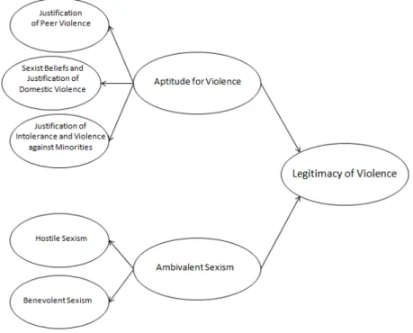
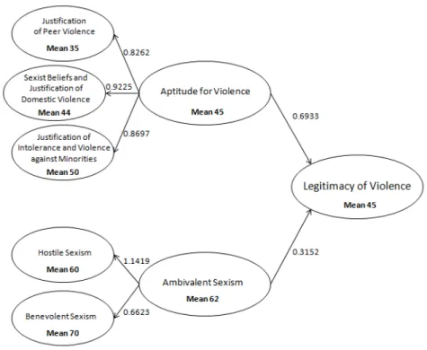
3.7 The third-orderLegitimacy of Violence construct . . . 88
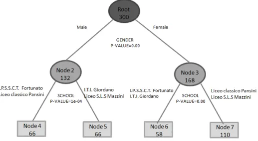
3.8 The estimated third-orderLegitimacy of Violenceconstruct . 91 3.9 PATHMOX Regression Tree . . . 93
3.10 Dendrogram of students . . . 96
3.11 Contribution of each LV to Legitimacy of Violence for each cluster . . . 98
3.12 Contribution of each LV to its own sub-dimensions for each cluster . . . 98
4.1 Types of Higher-Order Construct . . . 106
4.2 Model building: the Repeated Indicators Approach . . . 108
4.3 Model building: the Two Step Approach . . . 111
5.1 Second-Order Construct with all the MVs of the First-Order
Construct . . . 129
5.2 The scores of each Lower-Order Construct . . . 130
5.3 Second-Order Construct with the PLS scores of the First-Order Construct . . . 131
5.4 Second-Order Construct with all the MVs of the First-Order Construct . . . 135
5.5 Second-Order Construct with the PLS-R Component of the First-Order Construct . . . 136
5.6 Path diagram for the Higher-Order Construct . . . 138
5.7 Standard errors of the path coefficients . . . 141
5.8 Redundancy for the Second-Order LV . . . 143
2.1 A CI Decision Matrix . . . 50
3.1 LVs and MVs of the Social Cohesion model . . . 73
3.2 The outer estimation of the model . . . 75
3.3 Communality index for latent blocks for each estimated model 75 3.4 Path coefficients for each model . . . 76
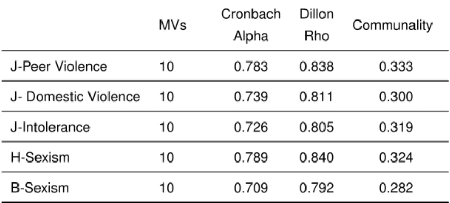
3.5 Reliability measures for Lower-Order Constructs . . . 89
3.6 Reliability measures for Higher-Order Constructs . . . 90
3.7 Path coefficients . . . 90
3.8 Codification of segmentation variables according to their type of scale and level . . . 92
3.9 F-global values and partitions - Least Squares Method . . . . 94
3.10 Coefficients estimate computed for each terminal node . . . 95
3.11 REBUS segments . . . 97
3.12 Quality measures . . . 97
3.13 Characterization of the LVs for each cluster . . . 99
3.14 Group Quality Index . . . 100
4.1 LVs and MVs of the Multidimensional Poverty CI . . . 118
4.2 Reliability Measures of the First-Order Constructs . . . 119
4.3 Reliability Measures of the Higher-Order MP-CI for each ap-proach . . . 120
4.4 Path Coefficients and t-statistics for each approach (non-significant parameters are marked in bold) . . . 121
4.5 Explained variance of the three approaches . . . 122
5.1 Path coefficients, bias and standard error for the inner model 140 5.2 RB of the path coefficients for each approach . . . 142 5.3 Redundancy for the Second-Order LV . . . 142 5.4 Reliability Measures of the Higher-Order MP-CI for each
ap-proach . . . 145 5.5 Path Coefficients and t-statistics for each approach (the most
significant blocks for each method are marked in bold) . . . 146 5.6 Global Measure of Goodness of Fit . . . 146 5.7 Ranking of countries according to the MP-CI scores based on
the Mixed Approach . . . 147 5.8 Ranking of countries according to the MP-CI scores based on
The real world is characterized by deep complexity. Many social, economic and psychological phenomena are manifold and therefore difficult to mea-sure and to evaluate. A phenomenon is defined as complex when the rele-vant aspects of a particular problem cannot be captured by using a single perspective [43]. It is necessary to consider the concept formed by different dimensions, each representing different aspects of it, which interact with each other. For this reason, most of the time, the complexity implies also multidimensionality [25], and this affects the measuring process of phe-nomenon that we are analyzing. Nowadays, phenomena such as Develop-ment, Progress, Poverty, Social Inequality, Well-Being, and Quality of Life, etc., require, in order to be measured, that the ‘combination’ of different dimensions are considered together as the proxy of the phenomenon. This combination can be obtained by applying methodologies known as Com-posite Indicator[100]; [69].
According to Saisana et al. [138], aComposite Indicator (CI) is defined as
a mathematical combination of single indicators that represent different di-mensions of a concept whose description is the objective of the analysis. CIs are very useful in order to deal with those phenomena that can not be observed directly.
The existing literature offers different alternative approaches in order to obtain a CI:Theory Based, obtained through the synthesis of selected Ele-mentary Indicators (EIs), and Data Driven, obtained through an optimal synthesis of a suitable set of EIs .Theory Based CIs, computed by aggrega-tion methods, usually require strong knowledge or assumpaggrega-tions about the
phenomena under study and consequently are constructed with a small number of variables. Data Driven CIs allow for the use of a large num-ber of variables that usually are needed in representing the real world, but they have an normative aim. Theory Based andData Driven approaches present several limitations: no explicit mention is made about the relation-ship between EIs and their own CIs (the reflective or formative measure-ment model); no predictive use of CIs is possible: their scope is essentially descriptive with, therefore, a restricted use in decision making processes; no systemic vision is considered in their building; no relationship with other CIs is taken into account; the CIs assume the same role, not distin-guishing between input, output and outcome variables; and the EIs are based just on a numerical scale. To overcome these restrictions, a Model Based CI can take into account a-priori knowledge on the field of interest by: specifying the CI measurement model (reflective, formative or both (MIMIC)); including any kind of CI relationship (logical, hierarchical, tem-poral or spatial); contextualizing the CI with respect to other CIs according to a given path model in a systemic vision; defining the roles of the CIs in the model; and in addition making use of non numerical data (ordinal and nominal) which is possible by suitable internal quantification according to optimal scaling methods.
In order to compute aModel Based CI, taking into account all a-prior in-formation, a relevant role is played by theStructural Equation Modeling (SEM) methodology. This is a statistical technique for testing and estima-ting causal relationships using a combination of statistical data and quali-tative causal assumptions. SEM [84] is an extension of the general linear model that simultaneously estimates relationships between multiple inde-pendent, dependent and Latent Variables (LVs). According to this metho-dology, it is possible to define a CI as a multidimensional LV not mea-surable directly and related to its single indicators or Manifest Variables (MVs) by a reflective or formative relationship, or both (this defines the measurement or outer model). Each CI is related to the other CIs, in a sys-temic vision, by linear regression equations specifying the so-called Struc-tural Model (or Inner Model). As a result a Systemic CI or a System of CIs
is obtained, where the word “systemic” derives from the definition of sys-tem given by Ludwig von Bertalanffy [96], according to which “a syssys-tem is a set of elements in interaction”, not just an aggregation of EIs, but a set of indicators related to each other by mutual relationships, expressed through functional links and summarized in a specific model.
Two different approaches exist to estimate model parameters in SEMs: the
covariance-basedtechniques [76];[77] and thecomponent-based techniques [186];[187];[95]. The first approach is primarily used to confirm (or re-ject) theories (i.e. a set of systematic relationships between multiple vari-ables that can be tested empirically). In contrast, incomponent-based tech-niques, LV (i.e CI) estimation plays a main role. As a matter of fact, the aim ofcomponent-based methods is to provide an estimate of the LVs in such a way that they are the most highly correlated with one another (according to the path diagram structure) and the most representative of each corre-sponding block of MVs.
Among the several methods that have been developed to estimate SEMs, we focus on thecomponent-basedtechniques, in particular on thePLS Path Modeling Approach (PLS-PM) [183]; [166], because the estimation of the CIs plays a key role in this estimation process.
The PLS-PM approach has enjoyed increasing popularity as a key multi-variate analysis method in various research disciplines in order to build a system of CIs. It has been evolving as a statistical modeling technique, with the results that there are several published articles on the method [166]; [16]; [57]; [64]; [35]. In Chapter two of the this the thesis PLS-Path Mod-eling Approach is reviewed, and a description of the PLS-PM algorithm, step by step, is proposed. PLS-PM allows you to estimate causal relation-ships, defined according to a theoretical model linking two or more latent complex concepts, each measured through a number of observable indica-tors. The basic idea is that the complexity inside a system can be studied by taking into account the entirety of the causal relationships among the LVs, each measured by several MVs. In this system, we are interested in including EIs on a non numerical scale, including some kind of CI relation-ship and testing whether there is a mediating and/or moderating effect.
For instance, when computing a CI, it could be interesting to consider de-mographic variables, such as religion or gender, and categorical variables defining states, such as the type of government. It would be interesting to know what the role of these variables is, if they have a moderator or medi-ator effect, and how considering these effects change thee estimation of the LVs considering these effects.
Moreover, applications of SEMs are usually based on the assumption that the analyzed data stem from a single population, so that a unique global model well represents all the observations. However, in many real world applications, this assumption of homogeneity is unrealistic. In modeling the real world, it is reasonable to expect that different classes showing het-erogeneous behaviors may exist in the observed set of units. This is true also in CI frameworks. As a matter of fact, in developing a system of CIs, it is reasonable to suppose that different models should be applied in order to take into account differences among the units. Therefore, in recent years there have been many advances in the context of these models, with many tools being developed in order to extend the classic algorithm of the PLS-PM to the treatment of non metric data, for including and testing mediator and moderator effects, and to deal with heterogeneous data. We have ad-dressed these developments in the third chapter of the thesis, focusing in particular on two approaches developed in recent years.
In the fourth chapter of the work we will focus on another aspect of PLS-PM concerning the construction of the hierarchical component model. As a matter of fact, in relation to the CI framework, researchers have recently been focusing their attention on a particular aspect linked to multidimen-sionality and a high level of abstraction, when a CI is manifold, lacks its own MVs and is described by various underlying blocks.
Higher-Order Constructs in PLS-PM are considered as explicit represen-tations of multidimensional constructs that exist at a higher level of ab-straction and are related to other constructs at a similar level of abstrac-tion completely mediating their influence from or to their underlying di-mensions [12]. In Wold’s original design of the PLS-PM [186] it was ex-pected that each construct would be necessarily connected to a set of
ob-served variables. On this basis, Lohmöller [95] proposed a procedure to treat hierarchical constructs, the so-called hierarchical component model. The hierarchical constructs or sayings are multidimensional constructs that involve more than one dimension and we can distinguish them from the one-dimensional constructs that are characterized by a single underlying dimension.
There are three main approaches existing in the literature: the Repeated Indicators Approach, the Two Step Approach and the Hybrid Approach. The Repeated Indicators Approach [95]; [186] is the most popular approach when estimating Higher-Order Constructs in a PLS-PM [175];[179]. The procedure consists of taking the indicators of the Lower-Order Constructs and using them as the MVs of the Higher-Order LV. The Two-Step Ap-proach is divided in two phases. In the first step the LV scores of the lower-order constructs are computed without the Second-Order Construct [122]. Then, in the second step, the PLS-PM analysis is performed using the com-puted scores as indicators of the Higher-Order Constructs. The Hybrid Ap-proach builds on an idea of Wold [186]. The idea behind this apAp-proach is to randomly split all the MVs of the lower-order constructs so that half are assigned to their respective construct and the other half are represented in the Second-Order Construct side [180]. Each approach presents some limi-tations, particularly two aspects which are taken into account in this work: the estimation of components for each block and the choice of the number of the components for each block.
In chapter five we focus on these particular aspects and we propose two new methods, called theMixed Two Step Approach and thePLS Compo-nent Regression Approach, that allow you to estimate the System of CIs differently and optimally. The Mixed Two Step Approach begins with the implementation of the PLS-PM in the case of the Repeated Indicators Ap-proach. In this way, the algorithm gives the scores of the Lower-Order Constructs. Next the scores of the blocks are used as indicators of the Higher-Order Construct, and at this point the PLS-PM algorithm is per-formed again. The PLS Component Regression Approach gives the pos-sibility of choosing manually the number of components of the block to
be extracted, or according to a criterion, through the use of PLS Regression. Once the components have been chosen, these will be MVs of Higher-Order Construct and the PLS-PM algorithm will be performed. Since the aim of PLS-PM is to estimate the relationships between the LVs, these approaches provide components that are at the same time representative of their blocks and predictive of the Higher-Order Construct.
Finally, we will show the functioning of the proposed algorithms (imple-mented in an R code) through a simulation study. The performance of the proposed methods in terms of the explained variability, predictiveness and interpretation is compared to the classic Two Step Approach, using artifi-cial data. Compared to this approach, theMixed Two Step Approach and the PLS Component Regression Approach seem to be good methods in term of stability and predictiveness. This is confirmed by the simulation and by an application to real data, that is presented in order to show the implementation of these methods and to give some comparative empirical results.
Composite Indicators
1.1
Introduction
The real world is characterized by deep complexity. Many socioeconomic phenomena are manifold and therefore difficult to measure and to evalua-te. A phenomenon is defined as complex when the relevant aspects of a particular problem cannot be captured by using a single perspective [43]. It is necessary to consider the concept formed by different dimensions, each representing different aspects of it, which interact with each other. For this reason, most of the time, the complexity implies also multidimensionality [25], and this affects the measuring process of the phenomenon that we are analyzing. As a matter of fact, outcomes are determined not by sin-gle causes but by multiple causes, and these causes may, and usually do, interact in a non-additive way. In other words the combined effect is not necessarily the sum of the separate effects. The Millennium Development Goals, adopted by the United Nations General Assembly in 2000, reflect this advanced vision. The shift from a single dimension to multiple di-mensions, by enlarging and enriching the scope of the analysis, represents an important theoretical progression.In last few years, the debate on the measurement of multidimensional phenomena has witnessed, within the worldwide scientific Community, a renewed interest thanks to the publica-tion, in September 2009, of the Stiglitz report and, in March 2013, of the first report on “Equitable and Sustainable Well-being” (BES) by the Committee
composed of ISTAT (the Italian National Institute of Statistics) and CNEL (Italian Council for Economics and Labour). It is well know that a number of socio-economic phenomena cannot be measured by a single descriptive indicator and that, instead, they should be represented with multiple di-mensions. Phenomena such as Development, Progress, Poverty, Social In-equality, Well-Being, Quality of Life, and the Provision of Infrastructures, etc., require, in order to be measured, that the “combination” of different dimensions are considered together as the proxy of the phenomenon. This combination can be obtained by applying methodologies known as Com-posite Indicator [100]; [69]. Once the multidimensionality is recognized, measuring this phenomenon has a number of theoretical and methodo-logical problems that are not present in the conventional unidimensional approach. The first problem concerns the choice of the dimensions: which and how many dimensions are relevant and should be considered or pri-vileged. This is also called by Sen the problem of the appropriate “infor-mational basis” [154], that is which information is included or excluded in the evaluation exercise. Moreover, we need to understand if there are relationships between these dimensions, and if so, to understand their na-ture. Therefore, in a multidimensional perspective and taking into account any relationships between the dimensions, we talk abouta system of Com-posite Indicators, that measure and represent distinct dimensions of the observed phenomenon. Consequently, the system of Composite Indicators does not represent a pure and simple collection of indicators but provides researchers with information that is greater than the simple summation of the elements.
1.2
Definition of Composite Indicators
Saltelli [139] used “Composite Indicator” (CI) sensu lato, i.e. to indicate a manipulation of individual indicators. Accordingly, a CI is obviously not “the unique solution” when representing complex systems but only “a solution”, (i.e. a limited exercise to take into account non-equivalent observers and observations). This is indeed the major limitation of com-posites. As indicated in Saisana et al. [137], the core of the non
aggrega-tors’ argument is in the subjective nature of these measures. Subjectivity cannot be avoided when representing complex systems. Cherchye et al. [11] observe that the “lack of consensus” is a defining property of CIs, and that one may even hypothesize a consensus between the association of key variables with the subject of the index, the weightings will remain contro-versial. However, several reviews of CIs have been published in the last few years. All this interest in CIs may be attributed to a variety of reasons, which could include the following ([138]; [110]):
- CIs can be used to summarize multidimensional issues, in view of the supporting decision-makers;
- CIs offer the possibility of making the rankings between, for example, countries, companies and individuals on complex issues;
- CIs can help to synthesize a list of indicators.
In official statistics, CIs are being increasingly recognized as a useful tool for policy making and public communications in term of conveying infor-mation about a country’s performance in fields such as the environment, economy, society, or technological development, and they have proven to be useful in ranking countries in benchmarking exercises. They are much easier to interpret than any attempt to find a common trend in many sepa-rate indicators. However, they can send misleading or non-robust policy messages if they are poorly constructed or misinterpreted. According to Saisana et al. [138], aComposite Indicator is defined as a mathematical combination of single indicators that represent different dimensions of a concept the description of which is the objective of the analysis. A CI is formed when individual indicators are compiled into a single index on the basis of an underlying model. CIs should ideally measure multidimen-sional concepts which cannot be captured by a single indicator, e.g. com-petitiveness, industrialization, sustainability, single market integration, or the knowledge-based society [138]. Thus, the main feature of a complex indicator is that it summarizes complex and multidimensional issues. This multiplicity implies a number of theoretical and statistical problems, espe-cially when we need to make comparisons over time and/or space. The
fundamental question is what is the best approach to (re)present complex phenomena and multidimensional realities. The construction of this kind of indicator implies a search for a suitable synthesis of a number of MVs in order to achieve a simple representation of a multidimensional phe-nomenon. Accordingly, a CI can be considered as a latent concept, not directly measurable, whose estimation can be obtained through the value of Elementary Indicators (EIs) or MVs. Its construction and its use involves a series of advantages and disadvantages, some of which are mentioned below. In particular, the principal advantages are that a composite indi-cator can be used to summarize multidimensional issues and can help to synthesize a list of indicators. On the other hand, the most serious pro-blems are that CIs may send misleading, non-robust policy messages, if they are poorly constructed or misinterpreted, and may encourage politi-cians to draw simplistic policy conclusions. These pros and cons are di-scussed in detail in Saisana et al. [138]. To overcome these problems, stu-dies in literature have focused on the construction of a CI through several stages that represent the basic steps of their construction, namely:
- Deciding on the phenomenon to be measured and on whether it would benefit from the use of CIs;
- Selecting the EIs. A clear selection needs to be made in terms of which sub-indicators are relevant to the phenomenon to be measured. There is no fully objective way of selecting the relevant EIs;
- Assessing the quality of the data. There needs to be high quality data for all the indicators. Otherwise, the analyst has to decide whether to drop the data or find ways of constructing the missing data points. In case of data gaps, alternative methods can be applied, e.g. mean substitution, correlation results, time series, or an assessment of how the selection of the method can affect the final result;
- Assessing the relationships between the sub-indicators. Methods such as Principal Components Analysis can provide an insight into the re-lationships between the EIs. It can be considered as a prerequisite for the preliminary analysis of the EIs;
- Normalising and weighting the indicators. Many methods for nor-malising and weighting the EIs are reported in the literature;
- Testing for Robustness and Sensitivity. Inevitably, changes in the weighting system and the choice of EIs will affect the results that the CI shows.
Each step is extremely important, but coherence in the whole process is equally vital. Choices made in one step can have important implications in others.
An OECD study [111] offers “recommended practices” for the construction of CIs [139]. In this book, Nando et al. [111] discuss in detail several stages for their construction, together with the “pros” and “cons” associated with the use of aggregated statistical information.
1.3
A quality framework for Composite Indicators
The development of a quality framework for CIs is not an easy task. In fact, the overall quality of the CIs depends on several aspects, related both to the quality of the elementary data used to build the indicator and the sound-ness of the procedures used in its construction. Quality is usually defined as “fitness for use” in terms of user needs. As far as statistics are concerned, this definition is broader than has been used in the past when quality was equated with accuracy. It is now generally recognized that there are other important dimensions. Even if the data are accurate, they cannot be said to be of good quality if, for example, they are produced too late to be useful, cannot be easily accessed, or appear to conflict with other data. Thus, qua-lity is a multi-faceted concept. The most important quaqua-lity characteristics depend on user perspectives, needs and priorities, which vary across user groups. Several organizations (e.g., Eurostat, the International Monetary Fund (IMF), Statistics Canada and Statistics Sweden) have been working on the identification of various dimensions of quality for statistical products. According to these organizations, the selection of basic data should max-imize the overall quality of the final result. In particular, in selecting the
data the following dimensions (drawing on the IMF, Eurostat and OECD reports) are to be considered:
Relevance. The relevance of the data is a qualitative assessment of the value contributed by these data. Value is characterized by the degree to which the statistics meet the current and potential needs of the users. It depends upon both the coverage of the required topics and the use of ap-propriate concepts.
In the context of CIs, relevance has to be evaluated by considering the ove-rall purpose of the indicator. A careful selection and evaluation of the basic data has to be carried out to ensure that the right range of domains is co-vered in a balanced way. Given the actual availability of the data, “proxy” series are often used, but in this case some evidence of their relationships with the “target” series should be produced whenever possible.
Accuracy. The accuracy of the basic data is the degree to which they cor-rectly estimate or describe the quantities or characteristics that they are de-signed to measure. Accuracy refers to the closeness between the values provided and the (unknown) true values. Accuracy has many attributes, and in practical terms it has no single aggregate or overall measure. Of ne-cessity, these attributes are typically measured or described in terms of the error, or the potential significance of error, introduced through individual major sources of error. An aspect of accuracy is the closeness of the initially released value(s) to the subsequent value(s) of the estimates. In light of the political and media attention given to first estimates, a key point of interest is how close a preliminary value is to the subsequent estimates. In this con-text it is useful to consider the sources of the revision, which include the replacement of preliminary source data with later data, the replacement of judgmental projections with source data, the changes in definitions or estimating procedures and the updating of the base year for constant-price estimates. The aim is few and only minor revisions; however, the absence of revisions does not necessarily mean that the data are accurate. In the context of CIs, the accuracy of the basic data is extremely important. Here the issue of the credibility of the source becomes crucial. The credibility
of data products refers to the confidence that users place in those products based simply on their image of the data producer, i.e., the brand image. One important aspect is trust in the objectivity of the data. This implies that the data are perceived to be produced professionally in accordance with appropriate statistical standards and policies and that practices are transparent (for example, the data are not manipulated, nor is their release timed in response to political pressure). All things being equal, data pro-duced by “official sources” (e.g. national statistical offices or other public bodies working under national statistical regulations or codes of conduct) should be preferred to other sources.
Timeliness. The timeliness of data products reflects the length of time between their availability and the event or phenomenon they describe, but considered in the context of the time period that permits the information to be of value and to be acted upon. The concept applies equally to short-term or structural data; the only difference is the time-frame. Closely related to the dimension of timeliness, the punctuality of data products is also very important, both for national and international data providers. Punctuality implies the existence of a publication schedule and reflects the degree to which the data are released in accordance with it.
In the context of CIs, timeliness is especially important to minimize the need for the estimation of missing data or for revisions of previously pu-blished data. As individual basic data sources establish their optimal trade-off between accuracy and timeliness, taking into account institutional, or-ganizational and resource constraints, data covering different domains are often released at different points of time.
Accessibility. The accessibility of data products reflects how readily the data can be located and accessed from original sources. The range of dif-ferent users leads to considerations such as multiple dissemination formats and the selective presentation of meta-data. Thus, accessibility includes the suitability of the form in which the data are available, the media of disse-mination, and the availability of meta-data and user support services. It also includes the affordability of the data to users in relation to its value to
them and whether the user has a reasonable opportunity to know that the data are available and how to access them.
In the context of CIs, the accessibility of basic data can affect the overall cost of the production and updating of the indicators over time. It can also in-fluence the credibility of the CI if a poor accessibility of the basic data makes it difficult for third parties to replicate the results of the CIs. In this respect, given improvements in the electronic access to databases released by va-rious sources, the issue of coherence across data sets can become relevant. Therefore, the selection of the source should not always give preference to the most accessible source, but should also take other quality dimensions into account.
Interpretability. The interpretability of data products reflects the ease with which the user can understand and properly use and analyze the data. The adequacy of the definitions of concepts, target populations, and variables, of the terminology underlying the data and of the information describing the limitations of the data, if any, largely determines the degree of inter-pretability. The range of different users leads to considerations such as the presentation of meta-data in layers of increasing detail. Definitional and procedural meta-data assist in interpretability.
In the context of CIs, the wide range of data used to build them and the dif-ficulties due to the aggregation procedure require the full interpretability of the basic data. The availability of definitions and classifications used to produce basic data is essential to assess the comparability of data over time and across countries: for example, series breaks need to be assessed when Composite Indicators are built to compare performances over time. There-fore the availability of adequate meta-data is an important element in the assessment of the overall quality of the basic data.
Coherence. The coherence of data products reflects the degree to which they are logically connected and mutually consistent, i.e. the adequacy of the data to be reliably combined in different ways and for various uses. Co-herence implies that the same term should not be used without explanation for different concepts or data items; that different terms should not be used
for the same concept or data item without explanation; and that variations in methodology that might affect data values should not be made without explanation.
In the context of CIs, two aspects of coherence are especially important: coherence over time and across countries. Coherence over time implies that the data are based on common concepts, definitions and methodology over time, or that any differences are explained and can be allowed for. Incoherence over time refers to breaks in a series resulting from changes in concepts, definitions, or methodology. Coherence across countries im-plies that from country to country the data are based on common concepts, definitions, classifications and methodology, or that any differences are ex-plained and can be allowed for.
1.4
Composite Indicators from different points of view
CIs have emerged in the last few years as an alternative to a portfolio of in-dicators, whose scattered information is sometimes difficult to grasp, an example being the GNP per capita, which often does not correlate well with development goals. As CIs have emerged, so they have also been criticized. Points of debate relate to the selection of dimensions and in-dicators, their correlation (and the trade-off between redundancy and ro-bustness), their type (input vs. output), and the normalization procedure, weighting, and aggregation of the components. Many services of the Euro-pean Commission, the United Nations and regional and local Institutions have been focusing on the development and use of Composite Indicators to convey concise information to the public about several economic, environ-mental, technological and social domains. CIs are deemed useful because they provide “the big picture”, they attract public interest and encourage the formulation of strong policy messages. However, their proliferation has been raising scepticism in relation to their accuracy and reliability. Given the seemingly ad hoc nature of their computation, the sensitivity of the results to different weighting and aggregation techniques, and the continu-ing problems of misscontinu-ing data, CIs can result in distorted findcontinu-ings on
coun-try performance and incorrect policy prescriptions [140]. The use of CIs is very much the subject of controversy, pitting aggregators against non-aggregators. Sharpe [155] notes that:
The aggregators believe there are two major reasons that there is value in combining indicators in some manner to produce a bottom line. They be-lieve that such a summary statistic can indeed capture reality and is mean-ingful, and that stressing the bottom line is extremely useful in garnering media interest and hence the attention of policy makers. The second school, the non-aggregators, believe one should stop once an appropriate set of in-dicators has been created and not go the further step of producing a com-posite index. Their key objection to aggregation is what they see as the arbitrary nature of the weighting process by which the variables are com-bined.
One may note that the controversy on the use of statistical indices unfolds along an analytical versus pragmatic axis. There is abundant literature on the analytical problems associated with even well-established statistical in-dices such as GDP [125]. This literature hardly seems to dent the GDP’s rather universal pragmatic practical acceptance. Along similar lines, in Saisana et al. [137], one reads:
[...]it is hard to imagine that debate on the use of Composite Indicators will ever be settled[...]official statisticians may tend to resent CIs, whereby a lot of work in data collection and editing is “wasted” or “hidden” behind a single number of dubious significance. On the other hand, the temptation of stakeholders and practitioners to summarize complex and sometime elu-sive processes (e.g. sustainability, single market policy, etc.) into a single figure to benchmark country performance for policy consumption seems likewise irresistible.
Among the list of objections to the use of CIs one reads [138]; [110]; [111]: - CIs may send misleading, non-robust policy messages if they are poorly
simplistic policy conclusions.
- The construction of CIs involves stages where judgment has to be made: the selection of the EIs, the choice of the model, the weighting of the indicators and the treatment of any missing values etc.
- There could be more scope for disagreement among Member States about CIs than about individual indicators.
- CIs increase the quantity of data needed because data are required for all the EIs and for a statistically significant analysis.
While the first “cons” is simply a reminder that sound practices must be used [111]; [137], and the last is an unavoidable consequence of complex-ity, the core of the non-aggregators’ argument rest in the subjective nature of these measures. Cherchye et al. [11], observe that the “lack of consen-sus” is a defining property of CIs, and that while one may hypothesize a consensus between the association of key variables with the subject of the index, the weightings will remain controversial. According to Nardo et al. [111]: CIs are much like mathematical or computational models. As such, their construction owes more to the craftsmanship of the modeler than to universally accepted scientific rules for encoding. As for models, the justifi-cation for a CI lies in its fitness for the intended purpose and its acceptance by peers[132].
The point of these considerations is that subjectiveness and fitness need not be antithetical. They are in fact both at play when constructing and adopt-ing a CI, where inter-subjectiveness may be at the core of the exercise, such as when participative approaches to weighting negotiations are adopted (see Nardo et al. for a review [111]). Thus, these only apparently conflict-ing properties underpin the suitability of CIs for advocacy. In discussconflict-ing data quality issues for statistical information Funtowicz and Ravetz note [44]:
Any competent statistician knows that “just collecting numbers” leads to nonsense[...]so in “Definition and Standards” we put “negotiation” as su-perior to “science”, since those on the job will know of special features and problems which an expert with only a general training might miss.
Concerning the discussion of the attraction exerted by CIs, an example is in the work of Amartya Sen, Nobel prize winner in 1998 [153]. Sen was initially opposed to CIs but was eventually seduced by their ability to put into practice his concept of “Capabilities” (the range of things that a person could do and be in her life[153]) in the Human Development Index. Saltelli adds that, however good the scientific basis for a given CI, its ac-ceptance relies on negotiation and peer acac-ceptance [139]. However, despite their many deficiencies, they will continue to be developed due to their use-fulness as a communication tool and, on occasion, for analytical purposes [138].
The evolution of CI theory has gone over the years more and more reflected on the production of the official statistics. Besides these, in the last few years a new vision has developed in all fields, many CIs have been built and used in order to deal with problems of synthesis of different latent con-cepts, particularly in economic and social fields. An obvious example is the construction of the ACSI (American Customer Satisfaction Index), in order to measure the Customer Satisfaction; a synthetic index that relates diffe-rent aspects, such as Expectation, Perceived Quality and Perceived Value, that go to influence the Customer Satisfaction.
1.5
From Data Driven Composite Indicators to Model
Based Composite Indicators
The construction of a CI implies the search for a suitable synthesis of a number of observed or MVs in order to achieve a simple representation of a multidimensional phenomenon. Accordingly, a CI can be considered as a latent concept, not directly measurable, whose estimation can be obtained through the values of EIs. There is a fundamental division in the indicators literature about indicators between those who choose to aggregate vari-ables into CIs and those who do not, and prefer using a suite of indicators. There is no doubt that composite indicators are appealing, especially as an answer to the calls for a replacement of the single indicator approach or the use of a suite of indicators, as for example the Human Development Index
(HDI) and GDP to measure progress. As a matter of fact, using a unique measure obtained by combining indicators can indeed capture reality and can easily be used to attract the attention of policy makers and the media. Moreover, the advantages of a composite indicator over a set of indicators include the creation of a bottom line. However, composite indicators have some disadvantages, including a danger that a composite index will over-simplify a complex system and give potentially misleading signals [58]. Accordingly, the selection of the weightings and the way the indicators are combined do not seem to be methodological but, rather, empirical issues in many approaches to the aggregation of indices. For the construction of CIs three different approaches [170] are proposed in the literature:
- Theory Based, obtained through the combination of some variables by means of a specified function, suggested by a theory or by well established knowledge on the phenomenon to analyze;
- Data Driven, obtained through a suitable/optimal synthesis of the selected variables, that represent the different facets of an analyzed phenomenon;
- Model Based, obtained by the estimation of a multi-equations model, describing, in an optimal way, not only the relationships among the observed variables but also between the observed variables and one or more of the latent constructs to be measured.
1.5.1 Theory Based and Data Driven Composite Indicators
Theory Based CIs are computed by simple formulas that usually combine a few observed variables. This approach requires strong knowledge or as-sumptions about the phenomena under study, and usually considers a well defined set of variables. In contrast, aData Drivenapproach overcomes the lack of knowledge by inserting into the building process of a CI many ob-served variables, that are only proxies of the concept to be measured. The absence of a prior knowledge and of a consolidated theory often necessi-tates the use of a data driven approach. This is an exploratory approach that falls into one of the five major principles of Benzecrì on which Data
analysis has to be based [8], according to which the models have to follow the data and not viceversa. Therefore, the statement of Benzecrì is reversed in the sense that the data have to follow the model in order to build not only descriptive CIs, but in addition to enrich new interpretations and their use in supporting decisions. A first step in the construction of a CI, according to the Data Driven Approach, consists in checking the coherence between the EIs and the concept to measure, in the sense that is all EIs must have a recip-rocal concordance (discordance) with respect to their relative CI. Suppose, for example, we want to build the “Quality of life” (QoL) CI that assigns a higher values to a country which enjoys a better quality of life: an indica-tor like “the income expected” has a positive correlation with the quality of life, whereas “infant mortality” usually presents an inverse correlation with the QoL. In order to have a set of coherent indicators we should trans-form it into the correspondence index “survival at birth”. The coherence can be simply achieved by calculating the reciprocal of an Elementary Indi-cator (EI) or by using its complement to the observed maximum value. In order to homogenize the different EIs, before their aggregation for the CI building, it is necessary to adopt a transformation in the same scale often of pure numbers. In this case, transformations for homogenization can be the following:
- a ranking transformation;
- a transformation by the sign of the difference with respect to the ref-erence mean;
- a transformation by the value of the ratio with respect to the reference value;
- a transformation by the percentage variation with respect to a previ-ous value; or
- a transformation by the standardization.
A transformation with respect to a reference value (i.e. the arithmetic mean, maximum or minimum value) must be carried out carefully when outliers are present in the EI distribution. In this case, a trimmed mean or defined
quartiles are to be preferred. Ones the EIs have been transformed into ho-mogeneity, the aggregation and the determination of a CI is achieved by the sum or an average of the values of the EIs for each statistical unit (e.g. a country). Some of the previous techniques have been used to build CIs at a European level, such as the Information and Communication Technologies index, the Scoreboard of DG Enterprise, the Internal Market Index and the Environmental Sustainability Index).
Alternative methods have been proposed in the literature [138] for building CIs according to the Data-Driven Approach, including Aggregation Tech-niques, Multiple Linear Regression Analysis, Principal Components Ana-lysis, Factor AnaAna-lysis, Cronbach’s Alpha and Neutralization of Correlation Effect.
Aggregation Techiques. Before computing a composite indicator, a trans-formation to homogenize the various elementary indicators is needed; next, an appropriate system of weightings on which the computation of a CI is based is defined, with methods that start from the simplest to the most com-plex. As an example, the Information and Communication Technologies Index is based on the simplest aggregation method: it involves ranking the countries for each EI and then adding together the country rankings. The Environmental Sustainability Index is based on the standardized scores for each indicator which equal the difference in the indicator for each country and the EU mean, divided by the standard error.
Multiple Linear Regression Analysis. This has been used to combine a number of EIs to compute correlation coefficients between all of the EIs. Linear regression models can tell us something about the linkages between a large number of indicatorsX1,X2, ...,Xn and a single output indicator
ˆ
Y. A multiple regression model is constructed to calculate regression coef-ficients that are the relative weightings of the EIs. This approach is used to build the National Innovation Capacity Index.
Principal Components Analysis. Applications of Principal Component Analysis (PCA) related to the development of composite indicators are
aimed at (i) identifying the dimensionality of the phenomenon (e.g. the Environmental Sustainability Index); (ii) clustering the indicators (the Gen-eral Indicator of Science & Technology); and (iii) defining the weightings (e.g. the Internal Market Index).
The PCA method has been widely used in the construction of CIs from large sets of indicators, on the basis of the correlation among EIs (e.g. the Internal Market Index, and the Science and Technology Indicator). In such cases, principal components have been used with the objective of combi-ning indicators into composite indicators to reflect the maximum possible proportion of the total variation in the set. The first principal component should usually capture sufficient variation to be an adequate representa-tion of the original set (e.g. the Business Climate Indicator). However, in other cases the first principal component alone does not explain more than 80% of the total variance of the EIs and several principal components are combined together to create the composite indicator (e.g the Success of Software Process Implementation, and the Internal Market Index).
Cronbach’s Alpha. Another way to investigate the degree of the correla-tions among a set of EIs is to use a coefficient of reliability (or consistency) called Cronbach’s Alpha α. This coefficient measures how well a set of variables (or indicators) measures the same underlying construct. A coef-ficient ofα= 0.80 or higher is considered in most applications as evidence that the indicators are measuring the same underlying construct. Cron-bach’s Alpha has been considered for example for the index of Success of software process improvement.
Neutralization of Correlation Effect. This method has been applied for the aggregation of three EIs into a composite indicator measuring the rel-ative intensity of regional problems of the Community by the European Community in 1984. The indicators measure a) GDP per employed in ECU, b) GDP per head in PPS, and c) unemployment rate. It is based on the strong correlation between the EIs, estimating a CI as an average of the EIs compared to their correlation.
The Data Driven Approach used in literature has some limitations with respect to the number of EIs used, to the choice of the system of weightings used to aggregate the EIs and to the absence of any relationship between the EIs and the CIs. As matter of fact, the current CI practice implies that the EIs:
- are based just on a numerical scale, no use being made of ordinal and nominal data with a consequent loss of precious information;
- assume the same role, with not distinction between input, output and outcome variables. The same applies to the moderating and mediat-ing variables whose use can improve the information carried by a CI; - no explicit mention is made of the relationship between the EIs and
their CI (the reflective or formative measurement model);
- no predictive use is allowed: their scope is essentially descriptive with, therefore, a restricted use in the decision making process. Besides, no systemic vision is considered in their building and no relation-ship with other CIs is taken into account. In order to overcome the previous restrictions a Model Based Approach has been proposed.
1.5.2 Model Based Composite Indicators
The previous section shows that the approaches proposed and used in lite-rature have some limitations with respect to the number of EIs used, to the choice of the system of weightings used to aggregate the EIs and to the ab-sence of any relationship between the EIs and the CIs. Midway between Theory Based and Data Driven CI approaches, theModel Based Approach allows you to take into account somea prioriinformation about the context of the phenomena by considering the relationship of the target or output CI with other CIs representing the input and outcome of the system under study in terms of a path diagram. In aModel Based Approach, a CI can take into account a priori knowledge of the field of interest by: i) specify-ing the CI measurement model (reflective, formative or both (MIMIC)); ii) defining the roles of the EIs in the model; iii) contextualizing the CI with
respect to other CIs according to a given path model in a systemic vision; and iv) including any kind of CI relationship (logical, hierarchical, tempo-ral or spatial).
In order to compute a Model Based CI, taking into account all a prior in-formation, a relevant role is played by theStructural Equation Modeling (SEM) methodology, where the computation of the weightings as well the aggregation process are not subjective. Both steps are based on the statisti-cal relationships between indicators. This is a statististatisti-cal technique for test-ing and estimattest-ing causal relationships ustest-ing a combination of statistical data and qualitative causal assumptions. SEM [84] is an extension of the general linear model that simultaneously estimates the relationships bet-ween multiple independent, dependent and LVs. According to this metho-dology, it is possible to define a CI as a multidimensional LV not measu-rable directly and related to its single indicators or MVs by either a reflec-tive or formareflec-tive relationship or by both (this defines the measurement or outer model). Each CI is related to other CIs, in a systemic vision, by linear regression equations specifying the so called Structural Model (or Inner Model). As a result a Systemic CI or a System of CIs is obtained, where the word “systemic” derives from the definition of system given by Ludwig von Bertalanffy [96], according to which “a system is a set of elements in interaction”, not just an aggregation of EIs but a set of indicators related to each other by mutual relationships, expressed through functional links and, summarized in a specific model.
The choice of using the SEM as the methodological framework is particu-larly useful for several reasons. Specifically:
- the possibility of obtaining, simultaneously and coherently with the estimation method, a ranking of individuals for specific indicator; - the possibility of comparing systemic indicators in space and in time; - the possibility of estimating the hypothesized relationships without
making assumptions about data distribution;
- the possibility of working with a large number of variables and a few observations;
- the possibility of estimating complex models without any problems of identification of the model;
- the possibility of working with missing data and in the presence of multicollinearity.
Two different approaches exist to estimate model parameters in SEMs: the
covariance-based[76];[77] techniques and theComponent-Based techniques [186];[187];[95].
The first approach is primarily used to confirm (or reject) theories (i.e. a set of systematic relationships between multiple variables that can be tested empirically). It does this by determining how well a proposed theoretical model can estimate the covariance matrix for a sample data set. In con-trast, in component-based techniques, the LV (i.e CI) estimation plays a main role. As a matter of fact, the aim ofcomponent-based methods is to provide an estimate of the LVs in such a way that they are the most strongly correlated with one another (according to the path diagram structure) and the most representative of each corresponding block of MVs. Among the several methods that have been developed to estimate SEMs we focus on theComponent-Based techniques, in particular on thePLS Path Modeling Approach (PLS-PM) [183];[166], because the estimation of the CI plays a key role in this estimation process. In the next Chapter, the PLS-PM is de-scribed and its properties and the advantages of using this approach for the estimation of a CI are highlighted.
Partial Least Squares Path
Modeling
2.1
Introduction
The Partial Least Squares (PLS) approach to Structural Equation Models (SEM), also known as PLS Path Modeling (PLS-PM) has been proposed as a component-based estimation procedure different from the classic covarian-ce-based LISREL approach. Herman Wold [181] first formalized the idea of partial least squares in his paper about principal component analysis. The first presentation of the finalized PLS approach to path models with LVs was published by Wold in 1975 [183] and other presentations of PLS-PM given by Wold appeared in the same year [182]; [184]. Wold [185] provides a discussion on the theory and the application of PLS for path models in econometrics. The main references for the PLS algorithm are Wold (1982) [186] and Wold (1985) [187]. Extensive reviews on the PLS approach to SEM with further developments are given in Chin [13] and in Tenenhaus et al. [166].
Wold opposed SEM-ML ([74]) ’hard modeling’ to PLS ’soft modeling’. The two approaches to SEM have been compared in Jöreskog and Wold [79]. PLS-PM is considered as a soft modeling approach, where no strong as-sumptions, with respect to the distributions, the sample size and the mea-surement scale are required. PLS-PM follows the SEM notations and
bols, including the use of a path diagram to picture the relationships among the LVs and between each MV and the corresponding LV. In the diagram, thepMVs are pictured by rectangles or squares, while circles represent the
qLVs. Arrows define the relationships among LVs and/or MVs.
As in SEM, in the PLS-PM, the overall relationships between the MVs and LVs are modeled through a system of equations. The goal of PLS-PM is not the reproduction of the sample covariance matrix, unlike the classic covariance-based approach. For this reason, PLS-PM is considered more an exploratory approach than a confirmative one: it does not aim to repro-duce the sample covariance matrix. [38]. Furthermore, PLS-PM provides a direct estimate of the LV scores.
2.2
The PLS path model
A PLS path model is made up of two elements, the measurement model
(also called the outer model), which describes the relationships between the MVs and their respective LVs, and the structural model (also called theinner model), which describes the relationships between the LVs. Both models are described in the next subsections.
2.2.1 The Measurement Model
An LVξis an unobservable variable (or construct) indirectly described by a block of observable variablesxkwhich are called MVs or indicators. There
are three ways to relate the MVs to their LVs:
- The reflective way (or outwards directed way); - The formative way (or inwards directed way);
- The MIMIC way (a mixture of the reflective and formative ways). -The reflective way
In the reflective way, each MV reflects the corresponding LV (Figure 2.1). A block is defined asreflectiveif the LV is assumed to be a common factor that reflect itself in its respective MVs. This implies that the relationship
Figure 2.1: Reflective model in a path diagram
between each MV xij (with i from 1 to q) and the corresponding LV is
modeled as:
xpq = λpqξpq+q (2.1)
whereξpq is the exogenous LV, andλpq is the simple regression coefficient
between the MV and the LV, the so calledloading.
In the reflective case, the MVs should be highly correlated, due to fact that they are correlated with the LV of which they are expression. In other words, the block has to be homogeneous. There are several tools for che-cking the homogeneity and unidimensionality of a reflective block:
- Cronbach’s Alpha;
- Dillon- Goldstein’s Rho; and
- Principal Component Analysis of a block.
Cronbach’s Alpha. A block is considered homogeneous if this index is larger than 0.7. αq= P p6=p0cor(xpq, xp0q) Pq+Pp6=p0cor(xpq, xp0q) × Pq Pq−1 (2.2)
wherePqis the number of MVs in the q-th block, andxpq andxp0qare two MVs of theq−thblock.
Cronbach’s Alpha is sensitive to the number of items in the scale and gene-rally tends to underestimate the internal consistency reliability.
Dillon- Goldstein’s Rho. This measures the composite reliability of the block. A block is considered homogeneous if its composite reliability is larger than 0.7. ρq = (PPq p=1λpq)2 (PPq p=1λpq)2+PPp=1q (1−λ2pq) (2.3)
According to Chin [13]Dillon-Goldstein’s Rho is considered to be a better indicator of the homogeneity of a block thanCronbach’s Alpha.
Principal Component Analysis rule. A block is considered homogeneous if, according to Kaiser’s rule, the first eigenvalue of the correlation matrix is higher than 1, while the others are smaller [166].
The first statistic assumes that each MV is equally important in defining the LV.
InDillon-Goldstein’sρ, in contrast, this assumption does not hold because it is based on the loadings of the model rather than the correlations ob-served between the MVs in the dataset. This type of reliability takes into ac-count the different outer loadings of the indicator variables.λpqsymbolizes
the standardized outer loading of the indicator variablei. The composite reliability varies between 0 and 1, with higher values indicating higher le-vels of reliability. It is generally interpreted in the same way as Cronbach’s Alpha. All of these rules assume, without any loss of generality, that LVs are standardized and all correlations between the MVs of the block show the same sign. In the case that the hypothesis of unidimensionality is re-jected, it is possible to identify some groups of unidimensional sub-blocks by considering the variable-factor correlations displayed on the loading plots. PLS-PM is a mixture of a priori knowledge and data analysis. In the reflective way, the a priori knowledge concerns the unidimensional-ity of the block and the signs of the loadings and the data have to fit this model. If they do not, they can be modified by removing some MVs that
Figure 2.2: Formative model in a path diagram
are far from the model. Another solution is to change the model and use the formative way.
-The formative way
In the formative case, the LV is supposed to be generated by its own MVs (Figure 2.2). ξq = Pq X p=1 ωpqxpq+δq (2.4)
whereωpq is the coefficient linking each MV to the corresponding LV and
δqis the error that represents the part of the LV not explained by the block
of MVs.
The assumption behind this model is the following predictor specification:
E(ξq |xpq) = Pq
X
p=1
ωpqxpq (2.5)
which implies that the residual vector E(δq) = 0and is uncorrelated with
the MVs. Each MV or every set of MVs represents a different level of the underlying latent concept. This model does not assume any homogene-ity or unidimensionalhomogene-ity of the block, and for this reason the block of MVs can be multidimensional and the indicators do not need to covary. Unlike reflective indicators, which are essentially interchangeable, high correla-tions are not expected between items in formative measurement models.
In fact, a high correlation between two formative indicators, also referred to ascollinearity, can prove problematic from a methodological and inter-pretational standpoint. When more than two indicators are involved, this situation is called multicollinearity. Collinearity may occur because the same indicator is entered twice or because one indicator is a linear combi-nation of another indicator. High levels of collinearity between formative indicators are a crucial issue because they have an impact on the estimation of weighs and their statistical significance, in particular boosting the stan-dard errors and thus reducing the ability to demonstrate that the estimated weights are significantly different from zero. High collinearity can result in the weighs being incorrectly estimated, as well as in their signs being reversed. To assess the level of collinearity, researchers should compute the
tolerance. Thetolerance represents the amount of variance of one forma-tive indicator not explained by the other indicators in the same block. It can be obtained in two steps:
1. first, we take the first formative indicatorx1 and regress it on all the
remaining indicators in the same block and calculate its proportion of variance associated with the other indicators (R2x1);
2. then, compute the tolerance for this indicator (T OLx1):
T OLx1 = 1−R2x1 (2.6)
A related measure of collinearity is theVariance Inflation Factor (VIF), de-fined as the reciprocal of the tolerance:
V IF = 1
T OLx1
(2.7)
A tolerance value of 0.20 or lower and a VIF value of 5 and higher respec-tively indicate a potential collinearity problem [57]. If the level of collinea-rity is very high, one should consider removing one of the corresponding indicators [55].