Localization for Autonomous Vehicles

(1)

Thesis for the Degree of Licentiate of Engineering

Localization for Autonomous Vehicles

Erik Stenborg

(2)

Localization for Autonomous Vehicles Erik Stenborg

c

_{Erik Stenborg}, 2017.

Technical report number: R012/2017 ISSN 1403-266X

Department of Electrical Engineering Signal Processing Group

Chalmers University of Technology SE–412 96 Göteborg, Sweden

Typeset by the author using LA_TEX. Chalmers Reproservice

(3)

Abstract

There has been a huge interest in self-driving cars lately, which is under-standable, given the improvements it is predicted to bring in terms of safety and comfort in transportation. One enabling technology for self-driving cars, is accurate and reliable localization. Without it, one would not be able to use map information for path planning, and instead be left to solely rely on sensor input, to figure out what the road ahead looks like. This thesis is focused on the problem of cost effective localization of self-driving cars, which fulfill accuracy and reliability requirements for safe operation.

In an initial study, a car equipped with the sensors of an advanced driver-assistance system is analyzed with respect to its localization performance. It is found that although performance is acceptable in good conditions, it needs improvements to reach the level required for autonomous vehicles. The global navigational satellite system (GNSS) receiver, and the automotive camera system are found to not provide as good information as expected. This presents the opportunity to improve the solution, with only marginally increased cost, by utilizing the existing sensors better.

A first improvement is regarding global navigational satellite systems (GNSS) receivers. A novel solution using time relative GNSS observations, is proposed. The proposed solution is tested on data from the DriveMe project in Göteborg, and found capable of providing highly accurate time-relative positioning without use of expensive dual frequency receivers, base stations, or complex solutions that require long convergence time. Error introduced over 30 seconds of driving is found to be less than 1 dm on average.

A second improvement is regarding how to use more information from the vehicle mounted cameras, without needing extremely large maps that would be required if using traditional image feature descriptors. This should be realized while maintaining localization performance over an extended period of time, despite the challenge of large visual changes over the year. A novel localization solution based on semantic descriptors is proposed, and is shown to be superior to a solution using traditional image features in terms of size of map, at a certain accuracy level.

(4)

List of appended papers

Paper I M. Lundgren, E. Stenborg, L. Svensson and L. Hammarstrand, "Ve-hicle self-localization using off-the-shelf sensors and a de-tailed map", 2014 IEEE Intelligent Vehicles Symposium, Proceed-ings pages 522-528.

Paper II E. Stenborg and L. Hammarstrand, "Using a single band GNSS receiver to improve relative positioning in autonomous cars", 2016 IEEE Intelligent Vehicles Symposium, Proceedings pages 921-926 Paper III E. Stenborg, C. Toft and L. Hammarstrand, "Long-term Visual Localization Using Semantically Segmented Images", Submit-ted to 2018 IEEE International Conference on Robotics and Automa-tion

(5)

Preface

More than four years ago, when I was about to start this project, I thought, "Localization is almost solved, and what little remains ought to be easy! Five years is way too much time allocated - what am I going to do after three years when the problem is solved, and the DriveMe cars are roaming the streets of Göteborg with my code in them?". Now, almost five years later, I’m very happy that I’ve reached this half-way milestone, that the Licentiate thesis marks, and I wonder if I’m ever going to make a dent in the mountain of work that remains until the problem really is solved.

I have learned a lot, though. I have learned that research takes time. I have learned that the path to success is full of failures that nobody sees, but the person who makes them. I have learned that all those failures is part of the process. And I have learned to appreciate the advice from those who have gone through the process, and emerged successfully on the other end, a little bit wiser than the rest of us who are in the middle of it.

I would like to show my gratitude towards my academic supervisors Lennart Svensson and Lars Hammarstrand for your advise, for your unwa-vering support, for our interesting discussions about both professional and other matters, and for all help I have received to reach this milestone. A very big thanks also to my industrial supervisor Joakim Sörstedt and my manager Jonas Ekmark for giving me this opportunity, for your enthusiasm, for your support of my work, and for believing in me. I would also like to thank Vinnova, Volvo Car Corporation and Zenuity for financing my work. Thanks to all friends and colleagues (both in the past and the present) in the signal processing and the image analysis groups at Chalmers, at the active safety department at Volvo and at Zenuity. Lunches and fika wouldn’t be nearly as entertaining without you. Special thanks to Malin, for helping me getting started when I first joined the group at Chalmers and for co-authoring the very first published paper with my name on it, to Carl for being such a rock and helping me with my present work, to Anders for being a good room mate and accepting my quirks (I apologize for shooting you the first day we met). Special thanks also to Karl, Abu, Maryam, Daniel, Samuel, Erik, Yair, and all the rest of you already mentioned, for proof reading or otherwise helping me with this thesis and the papers in it.

A warm thanks to my parents. Without you, I literally wouldn’t be here today. Finally, I would like to extend a very warm thanks to my beloved wife, Yoko, and to my lovely daughters, Lina and Hanna, for being such a wonderful family. I love you.

Erik Stenborg Göteborg, 2017

(6)

(7)

Paper III Long-term Visual Localization Using Semantically Segmented Images 89 1 Introduction . . . 89 2 Problem statement . . . 91 2.1 Observations . . . 91 2.2 Maps . . . 93 2.3 Problem definition . . . 93 3 Models . . . 93 3.1 Process model . . . 93 3.2 Measurement model . . . 94 4 Algorithmic details . . . 96 4.1 SIFT filter . . . 96 4.2 Semantic filter . . . 97

(9)

Contents 5 Evaluation . . . 99 5.1 Map creation . . . 99 5.2 Ground truth . . . 100 6 Results . . . 101 7 Discussion . . . 101

(10)

(11)

Part I

(12)

(13)

Chapter 1 Introduction

Autonomous vehicles have several advantages to vehicles which must be driven by humans, one being increased safety. Despite an increase in number of cars and total distance driven, traffic injuries has declined in Sweden [1] and the USA [2], from being the leading cause of death in age groups below 45, to "merely" being in the top ten [3]. To continue this trend, we increase the scope of traffic safety from just protecting passengers in case of an accident, to mitigating or preventing accidents before they happen. Based on studies such as [4], where it is noted that a vast majority of accidents are caused by human error, we can see that the largest potential to further increased safety, lies in letting technology assist drivers by automating the driving task, and thus creating self-driving cars.

Other reasons for self-driving cars are economy, as people can be more productive while on the road; equality, as blind and otherwise impaired people then can ride by themselves; and also environment, since the need for parking in cities could be reduced if all cars could leave by themselves after the rider has reached the destination.

Now, let us look into the problems we need to solve to make autonomous vehicles available. These problems include human factors, economy, legal liability, equality, morality, etc. This thesis focuses on technical problems, specifically those regarding precise localization. Economy and safety re-strict possible solutions, but apart from that, we can view the problem of localization independently. The technical problem of autonomous driving can be described as a function which maps sensor data to control signals for the car, primarily wheel torque for longitudinal acceleration and steering torque for turning the car. The rest which needs controlling in the car, e.g. controlling flow of fuel and air to the engine, is already solved.

There are several possible ways in which we can approach this problem of mapping sensor data to control outputs. One possibility is to decide on a sensor setup that seems reasonable, e.g., a set of cameras based on the fact

(14)

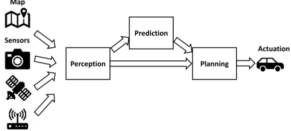
Chapter 1. Introduction Map Sensors Perception Prediction Planning Actuation

Figure 1.1: Flow of data and processing modules for autonomous driving. Localization is here considered part of the perception module.

that humans are able to drive a car mainly based on vision input, and then treat it as a machine learning problem, using either reinforcement learning or supervised learning with a human expert driver. This approach has so far rendered some success [5–7], but most larger scale projects are focusing on more modular approaches where the driving task is divided into smaller parts, which can be designed and verified more independently of each other. In the modular approach, the problem is subdivided into a few major modules, where Figure 1.1 shows one example of such a subdivision. We have one module which is responsible for planning a trajectory and following it based on information from the other modules, another which interprets the sensor inputs into a simple structure that is meaningful for the driving task, and a third which predicts what other traffic participants will do. The output from the perception block will typically contain information about both the dynamic environment, such as position and velocity of other road users, and the static environment, such as which areas are drivable and which contain static obstacles.

When it comes to describing the static environment, there are two paradigms. One is to rely only on the input provided by the sensors on the own car, and the other is to rely also on a predefined map and relating the sensor inputs to that map. The map paradigm will provide more in-formation about the static environment than what is visible using only the sensors, and is thus often preferred. However, to use a map, one must be able to localize the car in the map. Any uncertainty in position and orienta-tion in relaorienta-tion to the map will translate into uncertainty about the drivable area and in consequence also the planned path. Thus, we can see that

(15)

ac-curate localization in relation to an acac-curate map of the close surroundings of the car, is an enabler for autonomous driving.

Then what is needed to solve effective localization for autonomous ve-hicles? Firstly, we need to understand what is needed in terms of accuracy, availability and price. These requirements are far from obvious, and could warrant a thesis in and by itself, but a short description of how one can reason about it is included in Chapter 2. Secondly, we need a map that connects the observable landmarks with the possibly unobservable, static features of the road that are needed for path planning, i.e. drivable surface, static obstacles, etc. A few thoughts on this map have also been included in Chapter 2. Thirdly, we need sensors which are capable of observing the landmarks, and sensor models which describe how the observations relate to the physical world. In Chapter 3, radars are briefly described, while cameras and global navigation satellite systems such as GPS, are described in further detail, with a focus on how they can be used for localization purposes. Lastly, we need algorithms that combine the given maps and the measurements into estimates of position and orientation. This is achieved using the Bayesian estimation framework described in Chapter 4, where we see how to combine the models of various sensors with a motion model for the vehicle to arrive at probabilistic models of position and orientation.

This thesis examines what level of localization accuracy that can be achieved using different types of automotive classified sensors. It further establishes a few missing pieces in reaching desired performance, and pro-poses solutions for some of them. This is done in three separate papers, briefly summarized in Chapter 5.

(16)

(17)

Chapter 2 Localization

As concluded in the introduction, accurate localization with respect to a map is a key enabler for using information from those maps in the motion planner. In this chapter we start with a brief overview of the research area, then have a look at what goes in the map, then look at how to use the map for localizing with respect to the drivable area, and finish by reasoning about how to derive requirements on accuracy and availability.

1 Overview

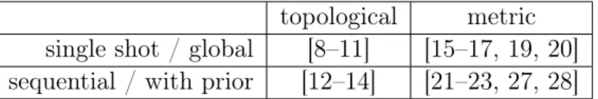
If we look at the problem of localization with a given map in a slightly larger context than for autonomous vehicles, we realize that it can be formulated in many different ways. We can roughly categorize problems in four categories, based on two criteria: metric vs. topological, and single shot vs. sequential. In Table 2.1, the references given below are categorized in either of the four categories.

The first division between metric or topological localization is regarding the result of the localization. Topological localization is when the result of localization is categorical and can be represented as nodes in a graph, e.g., a certain room in a house, or the location where an image from a training data set was taken. Examples here include place recognition by image retrieval methods, where an image database of geo-tagged images is used to represent possible locations, and then a query image is compared to the images in the database, and the most similar image along with its position is retrieved, see e.g., [8, 9]. Specialized loop closure detectors also belong in this category, see e.g., [10, 11]. These provide information to a larger system doing simultaneous localization and mapping (SLAM), when a robot has roughly returned to a previously visited place just by looking at image similarities. In this category, there are also some solutions which

(18)

Chapter 2. Localization

topological metric single shot / global [8–11] [15–17, 19, 20] sequential / with prior [12–14] [21–23, 27, 28]

Table 2.1: Classification of localization problems with a few examples of proposed solutions.

focus on robust localization in conditions with large visual variations, see e.g., [12, 13]. They make use of sequences of images which as a group should match a sequence of training images in an image similarity sense. One could also argue that some hybrid methods, such as [14], belong in this category, even though they claim to be "topometric" in the sense that they provide interpolation between the nodes in the graph and thus give metric localization result along some dimensions where a whole array of training images has been collected.

Metric localization is more geometric in nature. The resulting location is in a continuous space, and most easily expressed in coordinates using real numbers. There are examples from the computer vision community that does direct metric localization using a single query image, see e.g., [15–18], but also examples where a form of topological localization is performed first as an initial step, see e.g., [19, 20]. Most localization in robotics, with the purpose of providing navigational information to a robot, requires metric localization, with some examples in [21–23]. Localization using global satel-lite navigational systems and inertial measurement units are also examples of metric localization.

The second division we have when categorizing localization, is between single shot localization and sequential localization. This is regarding what type of information is used for the localization. Single shot localization uses only one observation and no additional information from just before or after. This is relevant when using single images, see e.g., [8, 9, 11, 15–20], and sometimes also when using sensors that are specialized for localization, such as the global navigation satellite systems, see e.g., [24].

Sequential localization means using a sequence of observations and some motion model to connect them, or alternatively, to have useful prior knowl-edge on the location from some other source. This is the type of observations available for on-line robot navigation, see e.g., [12, 13, 21–23, 25–28]. We note that the type of localization needed for autonomous vehicles falls in the intersection of sequential localization and metric localization. Thus, the rest of the thesis will focus on metric, sequential localization.

Localization for autonomous vehicles has been done for quite some time using expensive sensor setups, including survey grade GNSS receivers, fiber

(19)

1. Overview optical inertial measurement units and multi beam rotating laser scanners. Some of the most well known examples are the contributions to the DARPA Grand Challenge in 2005, see e.g., [25], and the DARPA Urban Challenge in 2007, see e.g., [26]. Some spin-offs from these DARPA challenges, such as Waymo, use similar technology, arguing that the cost of sensors will fall enough to make it viable for consumers in a near future. Others argue that more simple sensors should be enough for accurate and robust localization, but this is yet to be shown in practice. This cost constraint is the reason that this thesis is focused on solutions using sensors that are expected to be readily available in future cars.

Localization with a given map, and mapping given known positions and orientations, are considered subproblems to the more general problem of simultaneously estimating both location and map (SLAM). See e.g. [29, 30] for a survey of the SLAM problem. Although localizing with a given map would be sufficient for an autonomous vehicle, there is still a need to build the map and keep it updated. To keep costs down, this should should be performed without huge fleets of special mapping vehicles using very expensive positioning systems. Thus, viewing both the localization and mapping problems as SLAM problems is attractive from economical reasons, in spite of it being slightly more complicated.

In the 1990’s, SLAM was usually solved using extended Kalman filters, see e.g., [31, 32], where the state vector described the location of landmarks of the map and the most recent robot location. There were both convergence and scalability issues with this approach, due to a fixed linearization point, and an ever growing landmark covariance matrix that needed inverting in every update. In 2002, solutions using particle filters [33] were presented. They provided better performance for larger problems, due to not having to encode the correlation between landmarks, since they are conditionally independent given the robot trajectory. A few years later the trend shifted towards viewing the SLAM problem as a continuously growing smoothing problem, as in e.g., GraphSLAM [34], and iSAM [35, 36]. This is still how it is typically solved today, see e.g. [37, 38] for some more recent work. For people with a background in computer vision rather than robotics, it could be worth noting that, when using point features from camera images in GraphSLAM or iSAM, the solution is virtually identical to continuously solving a growing bundle adjustment problem with optimization methods that consider the sparse and incremental nature of the problem [39, 40].

(20)

2 Map representation

As previously noted, the problem in this thesis is self localization for au-tonomous vehicles using automotive grade sensors, and a map. For this we need a map, and although we have hinted that this can be solved using SLAM, it could be useful to discuss what to put in the map.

We know that the path planner needs some navigation information, e.g., drivable area, lane connectivity, traffic rules, suitable speed profiles, etc., to do its job. This navigational information is connected to positions in the world through markings on the ground, and traffic signs, which can be ob-served by a forward looking camera. These cues are what we would like to localize with respect to. However, some sensors, e.g., cameras looking backwards, radars, or GNSS receivers, can not directly observe them. In-stead we may choose to use some other observable landmarks, and encode their relation to the navigational information in the map. With a map that holds both the navigational information needed by the path planner, and observable landmarks, the car can use on-board sensors to detect angle and/or range to the landmarks, and triangulate a position relative to the navigational information in the map.

Now, these observable landmarks that we choose to add to the map can be quite sensor specific. Although geometric features, such as points or curves, are a popular choice, there are plenty of other options. One alternative is a grid map, where the world is discretized in a 2-D or 3-D grid, where each pixel (or voxel in the 3-D case) describes some property about that small part of the world. An often used property is occupancy, i.e., if the grid cell is transparent or opaque to the relevant sensor, often indicating that the cell is empty or occupied, hence its name [41, 42]. Another property that has been used successfully with grid maps is reflectivity, as in e.g., [43]. A version of grid mapping that has been popularized with the introduction of the Kinect RGB-D camera, is the truncated signed distance function. Here, each voxel stores the signed distance to the nearest opaque surface, if it is below some threshold distance. In indoor environments, where the size of the map is quite limited, 3-D grid maps have been demonstrated with impressive results. However, a grid representation of the world scales badly with the number of dimensions to be described, and although work has been done to compress the 3-D grids maps, see e.g., [44], most often this approach is used for 2-D maps.

For large 3-D maps, a more common approach is to store sparse features that are possible to describe with a few parameters. Points, lines, and B-splines are popular, but not the only possible choices. When using these types of features, we should take care to construct feature detectors that

(21)

3. Accuracy requirements are able to reliably detect these features in the sensor data.

Reference frame

For the motion planner, the only relevant information needed is the relative position from ourselves to other traffic participants, and to relevant objects in the immediate surroundings. Where the origin of the metric map of the world lies is irrelevant, as long as all relative positions and angles are correct. For most sensors, especially the cameras and radars used in this thesis, this is also true. However, GNSS provides global localization with respect to a certain origin of the Earth, and thus, if we want to use GNSS to localize in the map, the map must be aligned to the world origin as defined by the coordinate system used in GNSS.

Historically, maps have been thought of as 2-D projections of the surface of the Earth to a flat surface, such as a piece of paper or a screen. It is mathematically impossible to map the surface of a sphere to a plane without distortions and discontinuities, but there has been many proposals for suitable projections that does this without too much distortion, or with some special property preserved at the expense of some other error being introduced.

For our needs, however, we can drop the requirement that the map must project well to a 2-D plane. We are merely interested in using the map for localization and path planning, and for that we need to keep track of 3-D position of landmarks, and the road. The map must at least be able to store a 3-D representation of landmarks and the road, in any part of the world without discontinuities.

The most straight forward reference frame for a global 3-D map is an Earth centered and Earth fixed (ECEF) Cartesian coordinate frame that fol-lows the rotation of the Earth. In this coordinate system there are no prob-lems to map even Scott-Amundsen station at the south pole without discon-tinuities, and the transformation to a local east-north-up (ENU) frame is a simple rotation and translation. In the experiments in this thesis, however, the area where the car is driving is small enough, that a map in the local ENU frame, with a flat Earth assumption, is sufficient.

3 Accuracy requirements

Now, let us look into what performance we require of our localization. What accuracy of localization is needed for autonomous driving? How often and long can the localization be allowed to have an error over a certain threshold, and what is that threshold? These are difficult questions to answer, but in

(22)

order to evaluate performance, it is important to at least have an idea of the magnitudes, and a method to argue about them.

One possible starting point is a safety analysis. There are tools and frameworks to aid in such analysis, and they help us through hazard analysis and risk assessment to identify critical scenarios and the safety goals that arise from them. The hazards are classified according to their risk, which leads to a classification also of the safety goals. The ISO standard 26262 defines five Automotive Safety Integrity Levels (ASIL): QM, A, B, C, and D, with D being the highest level. The classification is based on how frequent the situation is (exposure), how severe the damages would be, and how controllable the situation is by the driver.

Let us take an example with the hazard of drifting out of the lane in a curve and colliding with oncoming traffic at 20 m/s or higher when in autonomous mode. This hazard is very severe in terms of expected dam-ages to the people involved in a head on collision, the situation is quite frequent (high exposure), and it has low controllability since the driver is not expected to be alert when the car is in autonomous mode. Thus, it gets the highest classification, ASIL D, which roughly translates to a desired fre-quency of error of less than 1 in 1000 years. Next, we can split the hazard into a fault tree, which should contain all possible faults that could cause it. There can be several possible causes, e.g., skidding if there is ice, not getting enough steering torque from the power steering, or lane information reported to the path planner being wrong. If the lane information is based only on using a map and localization, with ASIL D, both the map and the localization are required to give a lateral error that is small enough such that the vehicle does not cross over to the other lane (∼1 m).

This margin applies to the combined error of all components in the au-tonomous car, from sensing to actuation. To get the requirements for a specific module in the chain of modules presented in Figure 1.1, one could subtract the error introduced by the last module of the chain, and then propagate the remainder backwards through the various transformations that each block causes. Localization resides in the perception module, early in the chain, and this type of backwards propagation of permissible error could be quite cumbersome. A slightly less difficult way to get a rough understanding of the error margins, could be to simulate errors in the local-ization and propagate them forward to see what the final control error will be.

(23)

Chapter 3 Sensors and observations

When self-localization of cars is the topic, people often come to think of a Global Navigation Satellite System (GNSS), often the Global Positioning System (GPS), which has as its main purpose to measure position of the receiver. However, as we have seen, there are also other sensors, primar-ily used for other purposes, which can be quite useful also for localization. Cameras and radars, as examples of this type of sensors, are primarily used to detect obstacles and other road users in the local environment around the car, and often more than one of each is required to get a good enough un-derstanding of the surroundings. Together with GNSS, and motion sensors such as accelerometers, gyroscopes and wheel speed sensors, they provide the measurements that we use for localization.

So, how do these sensors work, and how do we use them for localization? One common factor is that they capture electromagnetic waves (light or radio) that was either transmitted or reflected by some object in the en-vironment. They typically record the angle of arrival, or measure distance to the object by recording the time delay of the captured signal. Some-times the intensity, and possibly some other features of the signal are also recorded. With sensors measuring angle to landmarks, the known positions of the landmarks can be used to triangulate the ego-position, see Figure 3.1. With sensors measuring distance, trilateration is used, see Figure 3.2. In both cases more than one landmark has to be detected to calculate an unambiguous position. In this chapter we look into more details on how the sensors used for localization in this thesis work, and how the measurements are modeled.

(24)

Chapter 3. Sensors and observations

1 landmark 2 landmarks

Figure 3.1: Triangulation from landmarks with known positions. With only one landmark, there is no unique solution, but with two landmarks we get a unique solution in 2-D.

1 landmark 2 landmarks

Figure 3.2: Trilateration from landmarks with known positions. With only one landmark, again there is no unique solution, and with two landmarks we get two possible positions in 2-D, but no information about orientation.

(25)

1. Global Navigation Satellite System

1 Global Navigation Satellite System

GNSS is, in a localization context, a rather unique sensor compared to other sensors. Its sole purpose is localization, while cameras and radars are primarily used in the self-driving car for their ability to detect obstacles and other road users. GNSS is also the only sensor which has a global frame of reference.

All GNSS systems, including GPS, which is the most well known, use the same principle of positioning. Kaplan and Hegarty describe this in detail in their book [45]. Essentially, a number of satellites with accurately known Earth orbits, transmit signals at very well defined times, and the receivers measure the delay from the transmission to the reception. From this delay the receiver can calculate the range to the satellite. By using multiple simultaneous satellite observations, the receiver is able to trilaterate its position.

Coarse/acquisition (C/A) code ranging

The signal that is transmitted from the satellite consists of a carrier signal, on top of which there are up to two other signals, modulated using Binary Phase Shift Keying. One of the signals is a repeating sequence of pseudo random numbers, which functions as a unique identifier for the satellite, and is also what is used for range calculations. The other signal, which is transmitted at a slower bit rate, is the navigational message. It pro-vides information about the satellite such as its status, orbital parameters, corrections to its clock, etc.

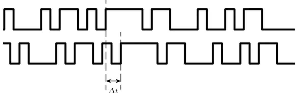
The normal method for determining position using GPS uses the se-quence of pseudo random numbers to calculate a pseudo range from the receiver to the satellite. Since the sequence of pseudo random numbers (C/A code) is known in advance by the receiver, this can be done with a tracking loop that calculates how much a local copy of the C/A code must be time shifted to match the received signal, see Figure 3.3. If the receiver had a perfect clock, and if smaller error sources are ignored, one could sim-ply multisim-ply the time shift with the speed of light to get the distance to the satellite. Given three such measurements to different satellites, the 3-D position of the receiver could be trilaterated. However, the clock in a typical receiver is of relatively low quality, which is why the receiver time must also be treated as an unknown variable. That increases the requirement to four satellites, in order to calculate a solution for position and time. This is the basic idea of how simple positioning using the C/A code in GPS works. If a receiver does not make use of the carrier phase to smooth the pseudo range measurements from the C/A code, there is a noise floor of around 1% of

(26)

Δt

Figure 3.3: The time offset, ∆t, when matching pseudo random numbers in the received C/A code signal to the internally generated sequence, is unique.

the bit length in the code, which is difficult to get below. The bit length is calculated as the bit length in seconds times the speed of light, and is around 300m. This means that the receiver tracking loop introduces noise on the pseudo range measurements that has a standard deviation of about 3m. However, since modern receivers use some tricks, such as carrier phase smoothing [46], the receiver noise is usually quoted as much lower today, see Table 3.1. Apart from the receiver tracking noise, there are other errors affecting the pseudo range measurements, leading to an average error that is typically quoted as around 7 m, for a standard single frequency receiver.

Carrier phase ranging

Now, consider the carrier signal, which has a wavelength of about 0.2 m; much shorter than the bit length of the C/A code. If the tracking loops in the receiver are able to determine the phase of the carrier signal within 1%, and if there is a way to remove additional errors, then potentially a very accurate range measurement to the satellite can be obtained.

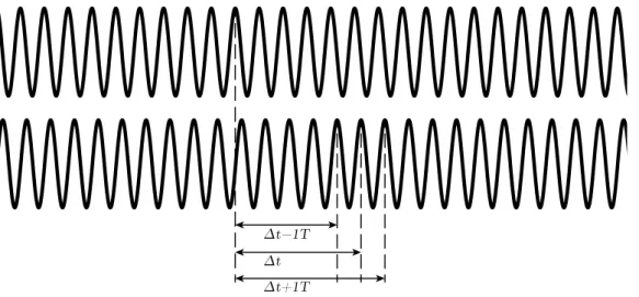
The alignment to the carrier phase through phase lock loops in the receiver, is indeed accurate to about 1 mm. However, there is now another problem. Every cycle of the carrier signal looks the same. This means that if we examine the cross correlation between the received signal and the internal oscillator, we would find an infinite number of peaks with a spacing that corresponds to the wavelength of the carrier signal. Which peak the phase lock loop locks on to, is random. This causes the range measurement using the carrier phase, to be offset by an unknown integerN times the wavelength. This integer, N, must be determined if we want to use the carrier phase range measurement as a normal range measurement, see Figure 3.4.

(27)

1. Global Navigation Satellite System

Δt−1T Δt+1T Δt

Figure 3.4: The true time offset,Deltat, when matching the received carrier signal to the internal oscillator, is not uniquely observable.

If we look a little bit deeper inside the receiver, we find that the phase tracking is not performed on the raw carrier signal, but instead on an inter-mediate frequency signal created by down mixing the carrier signal. When this intermediate frequency is 0 Hz, i.e., when the mixing signal has a fre-quency equal to the nominal frefre-quency of the carrier, it is easiest to analyze what is going on. If there was no relative range rate between receiver and satellite, the down mixed signal would be constant. When there is a relative range rate, the frequency of the mixed signal equals the Doppler shift of the carrier signal. The change in phase of this signal, multiplied by the wave length of the nominal carrier signal, equals a change in range to the satel-lite. Thus, we get a measurement of how much closer, or further away, the satellite is now, as compared to when the signal was first acquired. Instead of wrapping around every whole cycle, the phase should continue counting also the whole number of cycles since it locked on to the signal. This "un-wrapped" phase signal, counting number of whole cycles and the fractional part of the cycle, is what is considered the carrier phase measurement from the receiver.

In order to use the carrier phase measurements for localization, we need to solve the problem with the unknown integer of wavelengths between the receiver and satellite at the time phase lock was acquired. There are various methods for resolving this unknown variable when 5 or more satellites are visible and the conditions are otherwise good. The Least-squares Ambigu-ity Decorrelation Adjustment (LAMBDA) [47], is one popular method to resolve the integer ambiguity.

(28)

Error source Uncorrected Consumer receiver High end receiver Satellite clock 1.1 1.1 0.03

Satellite orbit 0.8 0.8 0.03

Ionosphere 15 7.0 0.1

Troposphere 0.2 0.2 0.2

Receiver noise N/A 0.1 0.01

Multipath N/A 0.2 0.01

Total N/A 7.1 0.2

Table 3.1: Standard deviation of user equivalent range errors (UERE) in meters for a typical consumer receiver using one frequency band [45], and a high end, dual frequency receiver using corrections for satellite errors.

Error sources

In addition to the limited accuracy of the phase lock loops, error in the estimated range to a satellite also comes from other sources. There is one family of errors that relate to the accuracy of the navigational message. Both the atomic clock of the satellite, and the position as given by the orbital parameters encoded in the navigational message, may be wrong by up to a few meters. The clock error, which is measured in seconds, is multiplied by the speed of light, in order to be comparable to other error sources.

On its way from the satellite to the receiver, the signal passes through the atmosphere, and this affects the time of arrival. In the ionosphere, the Sun radiation creates electrically charged particles that delay the signal. This delay varies with the time of day and some other factors. When the signal enters the more dense troposphere, there is yet another delay, which varies less than the ionosphere delay. Thus, it is more predictable when the altitude and weather conditions of the location are known.

Finally, there is multi path error, which is a local error caused by the signal reflecting from surfaces near the receiver. While all the errors above are strongly correlated in space, such that two receivers with a base line of up to a kilometer, experience almost the same satellite errors and atmospheric errors, the multi path error caused by reflections is not correlated when the receivers are more than a few meters apart.

Corrections of errors

All the errors above, with exception for the multi path, are possible to largely compensate for, because they change relatively slowly over time, and are spatially highly correlated. Corrections of the errors come in two

(29)

1. Global Navigation Satellite System different forms. Either one tries to model all parts and estimate them accurately from a few well known reference stations around the world, or one can bundle up all errors and correct the measurement directly with the help of a nearby reference station. The assumption in the latter case is that, if the base line between the receivers is short enough, then the total error at the two receivers will be almost identical. Thus, the errors will effectively cancel out, when taking the so called double difference [48].

The largest error source, the ionospheric delay, is inversely proportional to the carrier frequency, and thus, receivers that use two or more frequency bands can almost entirely eliminate this error. Single frequency receivers are restricted to rely either on a model of the ionosphere, or on the can-celing effect of a nearby base station. Rudimentary state space corrections are part of the base GPS system, in the form of coefficients to Klobuchar’s ionospheric model [49], and rough models of satellite clock and orbital pa-rameters. The WAAS/EGNOS/MBAS corrections provide more detailed ionospheric corrections, satellite clock corrections and satellite orbit param-eters. There are even more accurate corrections available with a delay of a couple of days from the International GNSS Service (IGS). Because of the delay, these corrections are more accurate than the on-line corrections, and thus, tend to be used in post-processing.

These corrections are used to a varying degree in receivers, depending on different design choices. Precise point positioning (PPP) is a technique that aims at resolving integer ambiguity of the carrier phase measurements by use of these corrections, but without the use of a nearby base state. In contrast, differential GNSS (D-GNSS) works with observation space cor-rections for the C/A code based pseudo range, and "real time kinematics" (RTK) is when observation space corrections are used to resolve carrier phase measurement ambiguities. The D-GNSS solution usually results in position estimates with error below 0.5 meters, while RTK with properly resolved integer ambiguity results in an error of a few centimeters. Observa-tion space correcObserva-tions are easy to apply, and converge quickly to an integer solution of the phase ambiguity when compared to state space corrections. However, they require a short base line (∼10km) to the base station to work, and are thus less suitable on the sea, or in other areas where there are no base stations around.

Configuration aspects for GNSS receivers

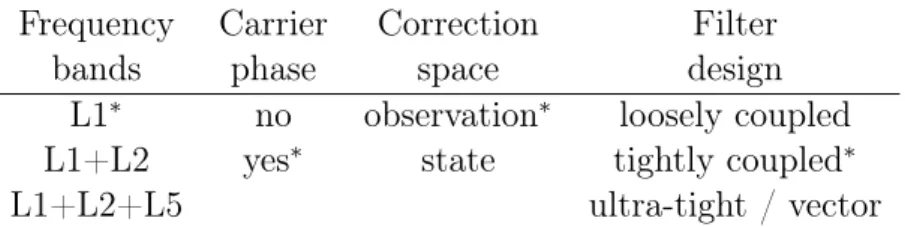
There are many aspects to consider in the design of a GNSS receiver which all affect the end performance and cost. Number of frequency bands will affect ionosphere error and speed of acquiring integer ambiguity resolution in RTK systems. Use of carrier phase enables high accuracy techniques such as

(30)

Frequency Carrier Correction Filter

bands phase space design

L1∗ no observation∗ loosely coupled L1+L2 yes∗ state tightly coupled∗

L1+L2+L5 ultra-tight / vector

Table 3.2: Configuration aspects for GNSS receivers. The asterisks mark the configuration used in Paper II.

RTK and PPP. Corrections can come either as state space corrections where each error source is estimated, or as observation space corrections where the observations of a nearby base station are subtracted from the mobile receiver observations to form single or double differences. Finally, the design of the localization filter where the GNSS measurements are combined with other position measurements from e.g., an Inertial Measurement Unit (IMU), can be coupled to various degrees. In a loosely coupled filter, the GPS receiver calculates a position/velocity/time (PVT) solution with no feedback from the position filter. The PVT solution provided by the receiver is then at some frequency, sent to the filter, where it is regarded as a measurement. A tightly coupled filter uses the pseudo ranges and phase information to each individual satellite, directly as measurements in the position filter. There they are combined together with measurements from IMU and other sources, as any other landmark measurement. One consequence of this is that, unlike in the loosely coupled filter, pseudo range measurements contribute to the position estimate even when there are only 2 or 3 visible satellites. In even more tightly coupled filters, the solution from the position filter is fed back into the tracking loops of the receiver. Thus, an IMU can help to reacquire the signal after short reception outages, or harden the receiver to spoofing. In Paper II we look at a specific configuration that has not been used much before, but offers a combination of low cost and high relative accuracy; see the combination marked with asterisks in Table 3.2.

2 Camera

Cameras are probably the most popular sensors to use with autonomous vehicles. They combine a low price with information rich measurements. One can also argue for the use of cameras by noting that humans can drive using only the same visual information that cameras capture, and that the road environment with traffic signs, lane markers, etc., is constructed with this in mind.

(31)

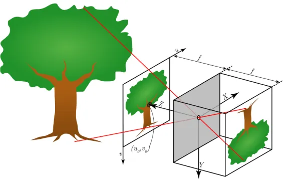
2. Camera u (u₀,v₀) Z X Y f v f

Figure 3.5: Pinhole camera projection of two points from an object, with image plane coordinate system (X, Y, Z), camera coordinate system (u, v), focal length (f), and principal point(u0, v0)marked.

Cameras typically do not emit any light, and relies on objects scattering light from various sources in the environment. They measure intensity of light in different angles from the focal point, but usually do not measure the range directly. As such, when using the camera for localization, we make use of several landmarks in the environment with known positions, measure the angle to them, and can then triangulate the ego position.

Pinhole camera model

To be able to use a camera in our localization process, we need a model which describes how the camera measurement, comprising the image pixels, relates to angles to objects. The camera sensor is essentially a grid of photo detectors where each one measures light intensity at a certain angle of incidence to the camera. The geometric relation between a light source in 3-D and the pixel on the flat image sensor which captures the light is modeled by the pinhole camera model in conjunction with a simple non-linear model for distortion [50].

Assuming the camera with focal length f is placed with the focal point (pinhole) in the origin, pointing along the Z-axis, and with the X-axis point-ing to the right, a 3-D point,[X, Y, Z]>, will project to the image plane at

(32)

[−f X/Z,−f Y /Z]> according to the pinhole camera model. This is under the assumption that the image plane lies behind the focal point as in the rightmost projection in 3.5. For convenience, we most often pretend that the image plane lies in front of the focal point, the leftmost projection in 3.5, to get an image that is not upside down, and thus get rid of the nega-tion, [f X/Z, f Y /Z]>. In the case of digital cameras, the image coordinate frame normally has its origin in one of the corners such that the point in the middle of the image is at position[u0, v0]>, leading to an offset in image coordinates as[f X/Z+u0, f Y /Z +v0]>.

This equation can be expressed conveniently when using homogeneous coordinates for both 3-D point, U =W[X, Y, Z,1]>, and the 2-D point in the image, u = w[u, v,1]>. We also need to loosen the assumption that the camera is located at the world origin, by introducing a rotation matrix from world coordinates to camera coordinates,R, and a translation vector,

˜

C, which gives the camera center in world coordinates. We then get the homogeneous camera coordinates as

u =PU (3.1) P=KR[I | −C˜] (3.2) K=   f mx 0 u0 0 f my v0 0 0 1  , (3.3)

where P is the complete camera calibration matrix, K is the intrinsic pa-rameter matrix,muandmv are conversion factors from metric units to pixel

units for the focal length, and u0 and v0 define the principal point of the camera given in pixel units. Having separatemu andmv allows for different

size of pixels in u (right) and v (down) directions.

Non linear distortion

For real cameras using optical lenses, the pinhole model is not particularly exact, but the errors can usually be described well with a relatively simple model. By combining the pinhole camera model with a non-linear distortion model, one can achieve sub-pixel accuracy. The distortion model we use is based on [50], and comprises two components: a radial distortion (3.6), and

(33)

2. Camera a decentering distortion (3.7), ˆ u=K   xd yd 1   (3.4) xd yd = xu yu +R+D (3.5) R= xu yu (κ1r2+κ2r4+κ3r6+. . .) (3.6) D = (2λ1xuyu +λ2(r2+ 2x2u)) (2λ2xuyu+λ1(r2 + 2y2u)) (1 +λ3r2 +λ4r4+. . .) (3.7) r =px2 u+y2u (3.8) w   xu yu 1  =R[I | −C˜]U, (3.9)

whereuˆ is the distorted point in the raw image, xd and yd are the

normal-ized distorted image coordinates, xu and yu are the normalized undistorted

image coordinates, R is the radial distortion, D is the decentering distor-tion, κi are the parameters for radial distortion, λi are the parameters for

decentering distortion, and w is the homogeneous scaling factor. Usually the distortion model is good enough using only κ1 and κ2, but often λ1,

λ2, and κ3 are also considered. These non-linear distortion parameters, to-gether with the parameters in K (3.3), are the intrinsic parameters of the camera. They are usually determined in a calibration procedure by maxi-mum likelihood estimation [51, 52]. With calibrated cameras, and assuming that the calibration stays constant over time, one only needs to determine the 6 free parameters of the camera pose for each image frame used in the localization. This is the procedure used in Paper III.

Image features

Now that we have a good model for how points in the world are projected to the camera image, we look into what we use the model for. The landmarks that we save in the map, must be possible to detect and localize in the images, and we do this using various feature detectors.

Typical examples of general image features are corner points, local min-ima or maxmin-ima of intensity, lines, or smooth curves. These features are often detected by looking at the gradient and finding where it is large (or 0 in the case of local extremal points), see [53] for an overview of general image feature detectors. These points or lines have no semantic meaning beyond

(34)

being points that are easy to detect and identify, and are quite general in the sense that they tend to work decently on most images, as long as the images are not extremely blurry or "smooth".

Often feature descriptors are used together with the detected features, in order to aid the data association (correspondence) between features at different time instances, or to landmarks in the map. There are many general purpose descriptors, e.g., SIFT [54], SURF [55], and BRIEF [56], which condense the local neighbourhood of a point in an image into a short vector which should be distinctive for this particular point. Again, these descriptors are general in the sense that they tend to work decently on most images.

Another approach to image features, is to detect features which have a special meaning to humans. In a road environment that could mean e.g., traffic signs, pedestrians, or lane markers. These detectors are harder to construct, but it is more obvious how the detections are useful in an au-tonomous car context, when compared to general feature points. Recent object detection algorithms are often based on supervised learning algo-rithms, specifically deep neural networks. These algorithms rely on having many manually labeled training examples to learn from. When that is available they have shown great performance, compared to hand engineered algorithms. These deep neural networks were first used to classify whole images, but also to detect interesting objects with bounding boxes within images. Recently there has been a surge in pixel wise classification, also called semantic segmentation. The task for a semantic classifier is to assign a semantically meaningful class, such as "human", "car", "building", etc., to each pixel in the image. With the introduction of fully convolutional networks [57], it is now possible to get quite good performance in this type of tasks, and one can see how it takes the bounding box approach one step further.

Automotive cameras detect and classify objects that are meaningful for the driving task, such as other vehicles, pedestrians, traffic signs, lane mark-ers, etc. Usually these features are detected and located in the image, but sometimes the detected positions are transformed into a vehicle coordinate frame. This transformation into 3-D can be achieved after capturing two or more frames and using visual odometry to triangulate the position of the object, or by using a flat world assumption, and knowledge about the mounting position of the camera on the vehicle. In Paper I we use only the lane marker descriptions from a camera of this type.

(35)

3. Radar

3 Radar

Radars work by illuminating objects with their own "light" source, and measure the time it takes for the signal to return, and can hence deduce the distance to the object. They emit radio waves in a beam which is swept over the scene of interest. Some older models used a physically moving antenna, but modern radars use electronically steered beams. The antenna elements are arranged such that by shifting the phase of the transmitted signal slightly, a beam can be directed in a selected angle. By steering this beam, the angle to objects can be measured. Besides angle, range and reflectivity of the objects are measured, and most often also the Doppler shift in the returned signal is measured, which means that the relative speed between the radar and the object can be determined. As with automotive cameras, automotive radars do further processing to detect peaks in the raw data which should correspond to the objects of interest. The radar usually also tracks and filters these detections over multiple frames before publishing the information on the data bus. Since the speed of the vehicle relative to the ground is estimated relatively well by the wheel speed sensors, and the relative speed to a target is measured by the radar, it is possible to extract the stationary objects for use in the localization process, while disregarding the moving objects, which are not of interest for localization purposes. Traffic signs and other metallic poles, such as the ones holding up side barriers, are typical examples of objects that are both stationary and good radar reflectors, and thus, of interest as landmarks in a radar map.

In contrast to camera images, the detection from a radar contain rela-tively little information. There is, to our best knowledge, no way to produce an effective descriptor for the radar detections. Thus, it will be much harder to match radar detections over time, or to a radar map. One way of han-dling the measurement to map association is presented in Paper I, but there are many other possible solutions to the data association problem, see e.g., [58–61].

(36)

(37)

Chapter 4 Filtering and smoothing

Bayesian filtering and smoothing are tools which are very useful for the task of localization. They can be used to answer questions such as, "What is the most likely location of the car, when taking into account all measure-ments that we have done up until now?" or "How certain is this estimated location?".

The word "Bayesian" in "Bayesian filtering" means that we make use of Bayes’ rule to update our belief of some state as we collect more mea-surements. This belief is expressed as a probability density (or probability mass function in the case of discrete variables), and is exactly what we use to answer questions about most likely value or uncertainty about some variable.

"Filtering", in this context, means that we have a sequence of noisy measurements from our sensors, and are interested in recursively estimating some state (e.g. the current location and orientation of a car), making use of all past measurements to infer this state. This is in contrast to "smoothing" where we are looking at the problem in an off-line setting, and thus also future measurements are available for all but the very last time instance.

An example of the on-line filtering setting, is the localization necessary for autonomous driving. The current location of the vehicle is most relevant for planning and control but the location one hour ago is not that useful. On the other hand, creating a map of the static environment around the road, is an example where smoothing makes more sense. Then, we are interested in creating the best possible estimate of the positions of landmarks, and we would like to use all available data. However, it is not critical to make the estimation on-line while recording the measurements. We may just as well save all the data and process it afterwards, when we return to the office.

(38)

Chapter 4. Filtering and smoothing

1 Problem formulation and general solution

Let us define the state that we are interested in estimating as a vector of real numbers, xk ∈ Rn, and the measurement we receive at time tk as

another vector, yk ∈ Rm. The subscript k denotes the k:th measurement

which is taken at timetk. One measurement sequence consists ofT discrete

measurements, which means thatk ∈[1, . . . , T]and thatj < k =⇒ tj ≤tk.

We can now define filtering as finding the posterior density, i.e., the density over possible states after all available measurements have been accounted for, p(xk|y1:k), and smoothing as p(x1:T|y1:T). Here, y1:k is short notation

fory1,y2, . . . ,yk, and T is the last time instance in the sequence.

To find the posterior density, we make a few simplifying assumptions. One assumption is that the current measurement yk when the

correspond-ing state xk is given, is conditionally independent of all other states and

measurements. Another assumption is that the state sequence is Marko-vian, which means that state xk when given state xk−1 is conditionally independent of all previous states,

p(xk|x1:k−1,y1:k−1) =p(xk|xk−1) (4.1)

p(yk|x1:k,y1:k−1) =p(yk|xk). (4.2)

Density (4.1) captures the uncertainties in the state transition, and (4.2) captures the relation between the measurement and the state. The same relations can also be expressed as

xk=fk−1(xk−1,qk−1) (4.3)

yk=hk(xk,rk), (4.4)

whereqk andrkare random processes, describing the error or uncertainty in

the models. As (4.3) models the procession of states over time, it is called a process model, or motion model when the state involves position. Similarly, (4.4) models the measurements, and is called a measurement model.

When we have restricted the class of problems to Markovian processes with conditionally independent measurements, the filtering and smoothing problems can be solved with recursive algorithms. In the filtering case, there is a forward recursion, whereas in the smoothing case, there is also a backward recursion. The base case in the filtering solution is for k = 0, when we have no measurement, and we base our solution solely on any prior knowledge we may have, summarized in p(x0).

The forward recursion step is then split in two parts: a prediction us-ing the process model, and then an update usus-ing the measurement model. Assuming we have a solution for p(xk−1|y1:k−1) from the previous time in-stance, we can now express p(xk|y1:k) in terms of already known densities

(39)

2. Kalman filter with the help of Dr. Kolmogorov and Reverend Bayes as

where the denominator in (4.7) is constant with respect to the state variable

xk.

As mentioned, smoothing can also be done recursively in two passes, where the first forward pass is identical to the filter recursion, and then a backward pass. The base case for the backward recursion is the final state atk =T, where the smoothing solution is identical to the filtering solution, p(xT|y1:T). Then assume that we have the smoothed solution at timek+ 1,

p(xk+1|y1:T) and now the task is to express p(xk|y1:T) in already known

In (4.11) we see the motion modelp(xk+1|xk), the filtering densityp(xk|y1:k),

the smoothing density from the previous stepp(xk+1|y1:T), and the filtering

prediction densityp(xk+1|y1:k), all of which are available from before.

2 Kalman filter

If the errors qk and rk from (4.3) and (4.4) are additive, normally

dis-tributed, and independent over time, and the models in themselves are linear, then we can solve the filtering and smoothing problems optimally, in a mean square error sense, using a Kalman filter [62]. All the assumptions regarding the process noise are seldom correct, but it is still a useful simpli-fication which works often enough. Also, there is seldom a need for having different models at each time instance. Then the simplified models are

(40)

xk =Fxk−1+qk−1, qk−1 ∼ N(0,Q) (4.12)

yk =Hxk+rk, rk∼ N(0,R), (4.13)

where F is the linear process model in matrix form, H is the linear mea-surement model in matrix form, and Q and R are the covariance matrices for the process noise and the measurement noise, respectively. Under these assumptions, the posterior distributions for both the filtering problem and the smoothing problem are also Gaussian, and can be exactly represented by their mean and covariance. The Kalman filter calculates mean, µˆ_k_|_k, and covariancePk|k, of the posterior density for each time step,k, with the

Hereµˆ_k_|_k is the estimated mean at time instancek using measurements up to, and including timek, whileµˆ_k|k−1is the predicted mean at time instance

k using measurements up to, and including time k−1, yˆk is the predicted

measurement, Sk is the predicted measurement covariance, and Kk is the

Kalman gain, all at time k.

The optimal smoothed solution can be achieved by first applying the Kalman filter, and then applying the Rauch-Tung-Striebel smoothing re-cursion [63], starting fromk =T −1 as

Gk=Pk|kF>P−_k₊₁1 |k (4.21)

ˆ

µ_k_|_T = ˆµ_k_|_k+Gk( ˆµk+1|T −µˆk+1|k) (4.22)

Pk|T =Pk|k+Gk(Pk+1|T −Pk+1|k)G>k. (4.23)

3 Unscented Kalman Filter

In many problems either, or both, of the process and measurement models are non-linear, in which case there is usually no exact solution. One com-mon solution, when the non-linearities are relatively mild, is to linearize

(41)

3. Unscented Kalman Filter the functions using Taylor series expansion at the estimated mean. This results in the posterior being approximated as a normal distribution, and the algorithms to calculate it, are the Extended Kalman filter (EKF) [64, 65] and Extended Rauch-Tung-Striebel smoother (ERTS), respectively.

Another option, which is used in the appended papers, is the sigma point methods, such as the Unscented Kalman Filter (UKF) [66] and the Cuba-ture Kalman Filter (CKF) [67]. These methods also approximate the pos-terior as a normal distribution, but in a slightly different way than through Taylor series expansion. One can think of the UKF and CKF in terms of numerical differences and view them as approximations to the EKF, but that is somewhat unfair, since both UKF and CKF generally approximate the densities involved better than what the EKF does [68]. The Unscented transform, which is the basis of the UKF, estimates the mean and covari-ance ofy=h(x)wherexis a normally distributed random variable, by first selecting a set of sigma points, X(i)_{, around the mean of} _x_{. These sigma} points are then propagated through the non-linear function, resulting in another set of sigma points, Y(i)_{. Then, the mean and covariance of} _y _can be approximated fromY(i) _{as a weighted sum.}

The UKF recursion which approximates the posterior density as a nor-mal distribution, is then given in terms of its approximated mean,µˆ_k, and covariancePk for each time stepk. First determine the sigma points,

X_k(0)₋₁ = ˆµ_k₋₁ (4.24) X_k(i₋)₁ = ˆµ_k₋₁+√n+κ p Pk−1 i (4.25) X_k(₋i+₁n) = ˆµ_k₋₁−√n+κ p Pk−1 i , (4.26)

then the prediction density,

(42)

Chapter 4. Filtering and smoothing then the posterior density,

all with weights as

W(0) = κ

n+κ (4.37)

W(i) = 1

2(n+κ), i= 1, . . . ,2n. (4.38)

Here n is the dimensionality of the state, κ is a tuning parameter, √P

denotes any matrix square root such that √P√P> = P, and

·

i selects

the i:th column of its argument. The special case when κ = 0 turns the UKF into CKF, which is used in Paper II.

In cases where the noise is not additive, it is possible to augment the state vector with noise states and use the same updates of the UKF or CKF filters [69].

4 Particle filters

Both the EKF and UKF approximates the posterior density as a normal density. Sometimes this approximation can be too crude. This may happen e.g., when the process model or the measurement model is highly non-linear, or it is known that the posterior density is multi-modal, and this needs to be reflected in the filtering solution. One possible solution when this is the case, is through multiple hypotheses filters [70–72], which describe the posterior as a sum of several normal distributions. Another popular solution is the particle filter, which makes no parametric approximation of the posterior density, but instead describes the posterior distribution as a weighted sum of many Dirac delta functions.

(43)

5. Smoothing and mapping When using a particle filter, we draw N samples, x(i)_{, from a proposal} distributionq(x0:k|y1:k)and assign a weight w(i) to each sample, where

w_k(i)= p(x0:k|y1:k)

q(x0:k|y1:k)

. (4.39)

Now the posterior distribution can be approximated as

p(x0:k|y1:k)≈ 1 N N X i=1 w(_ki)δ(x0:k−x(_0:i)_k). (4.40)

For the recursive step, assume that we have x(_0:i)_k₋₁ and w(_ki₋)₁ from the pre-vious step. The new set of samples at step k is drawn from the proposal distribution and gets weights as

x_k(i) ∼q(xk|x_0:(i)_k₋₁,y1:k) (4.41) w_k(i) ∝ p(yk|x (i) k )p(x (i) k |x (i) k−1) q(x(_ki)|x_0:(i)_k₋₁,y1:k) w(_ki₋)₁. (4.42)

The version of particle filters that is used in Papers I and III, called the bootstrap particle filter [73], uses the motion model as proposal distribu-tion, q(x(_ki)|x(_0:i)_k₋₁,y1:k) = p(x(_ki)|x(_ki−)1), which makes for a particularly easy recursion, x(_ki) ∼p(xk|x (i) k−1) (4.43) w(_ki) ∝p(yk|x (i) k )w (i) k−1. (4.44)

After the new samples are drawn and the weights are updated, the weights should be normalized such thatP

iwi = 1 over time. Due to the possibility

of particle depletion, i.e. most ofwi are almost zero, the samples need to be

resampled periodically. The resampling creates multiple copies of samples with large weights, and removes samples with near zero weight, and then resets the weights of the resampled particles.

5 Smoothing and mapping

Bayesian smoothing of a Markov process can be done optimally in a forward pass, followed by a backwards pass as seen in (4.11). However, for a typical mapping problem the Markov property does not hold, because when one returns to a previously visited place and recognizes this (loop closure), a direct dependence from that earlier time to now is created.

(44)

x

₁

y

₁

y

₄

y

₃

y

₂

x

₂

l

₂

l

₁

x

₃

x

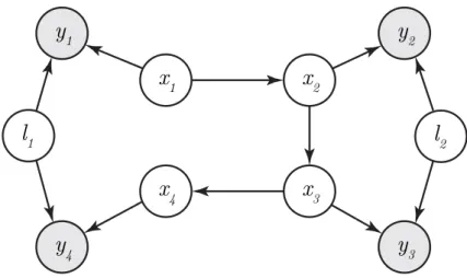
₄

Figure 4.1: Bayes net representation of a small SLAM problem with 4 robot poses, 2 landmarks, and 4 observations. Unknown variables are white, while given measurements are marked gray.

Let us create a small example that shows the problem. Assume that we have two landmarks,l1 and l2, that we are interested in mapping. We drive near them with a robot, and make noisy observations with a sensor on the robot. Our problem now, is that we do not know exactly the positions and orientations of the robot during the measurement campaign. Let us assume that the robot has made four measurements, y1, . . . , y4, of the landmarks from four different positions,x1, . . . , x4. Letl1 be seen fromx1 and x4, and

l2 fromx2 andx3. The corresponding Bayes network is shown in Figure 4.1. The relation between the posterior density of interest p(l1, l2|y1:4) and the measurement modelsp(y1|x1, l1)and p(y2|x2, l2)can be seen by introducing the x:s in the posterior density,

p(l1, l2|y1:4) =

Z

p(l1:2, x1:4|y1:4)dx1:4. (4.45) Now, the joint density inside the integral can be factorized in terms of motion model and measurement model.

p(l1:2, x1:4|y1:4)∝p(y1|x1, l1)p(x2|x1)

p(y2|x2, l2)p(x3|x2)

p(y3|x3, l2)p(x4|x3)

p(y4|x4, l1) (4.46) The landmarks, especially l1 which appears together with x1 to x4, pre-vent us from solving this with forward-backward smoothing. Therefore, we have to fall back to iterative methods. The iterative method could be for

Localization for Autonomous Vehicles