Housing prices and the public disclosure of flood risk: a
difference-in-differences analysis in Finland
© Springer Science+Business Media New York 2015, published by the Journal of Real Estate Finance and Economics at http://link.springer.com/article/10.1007/s11146-015-9530-3
This is the Final Draft version of the article for self-archiving purposes, according to Helsinki University’s Open Access policy and the Publisher’s self-archiving rules.
Athanasios Votsis 1 2 *, Adriaan Perrels 1
1 Socio-economic Impact Research, Finnish Meteorological Institute, Erik Palménin Aukio 1,
P.O. Box 503, FI-00101 Helsinki, Finland
2 Department of Geosciences and Geography, University of Helsinki, Finland
* Corresponding author; e-mail: [email protected], telephone: +358 50 4330789
Abstract: Information gaps and asymmetries are common in the housing market and this is frequently the case with the risks of natural processes, especially in coastal areas where the amenity dimension may dominate the risk aspect. Flood risk disclosure through maps is a policy instrument aimed at addressing this situation. We assess its effectiveness by identifying whether such maps induce a price differential for single family coastal dwellings in three Finnish cities, and by estimating the discount per square meter for various flooding probabilities (return times). The estimations indicate a significant price drop after the information disclosure for properties located in flood-prone areas as indicated by the maps. In the case of sea flooding information in Helsinki, the price effect is sensitive to the communicated probability of flooding. Overall, the discussed policy instrument appears to have functioned as intended, correcting information gaps and asymmetries related to flood risk. The identified effect is spatially selective; it caused a short-term localized shock in market prices in conjunction with some reorientation of demand from risky coastal properties towards ones that represent a similar level of coastal amenity, but are less risky in terms of flooding. This hints at the potential for incorporating the shocks associated with flood events or risk information into broader-scoped urban modelling and simulation. Similarly, the reasonable accuracy with which the housing market processes the additional information shows a potential for wider use of the disclosure of non-obvious risks in real estate markets. In the case of adapting to climate change risks, additional uncertainties may make the disclosure instrument less effective, if used as a single tool.
Keywords:flood risks, housing market, information effect, information gaps
Funding: This study was funded by the Academy of Finland as part of the RECAST project (decision number 140797) and by Helsinki University Centre for Environment (HENVI) as part of the ENSURE project.
Conflict of Interest: The authors declare that they have no conflict of interest.
Acknowledgements: We are indebted to Mikko Sane at the Finnish Environment Institute (SYKE) for providing the GIS files of the flood maps and Johannes Bröcker at the University of Kiel for advice in conceptualizing the study. We also thank the anonymous referees of this journal for the valuable comments provided.
1 Introduction
Housing constitutes a complex good that represents a basket of mutually substitutable attributes. Hedonic price estimations are widely used to decompose the price of housing into the marginal values of its traits (Rosen 1974; Dubin 1988; Sheppard 1999; Brueckner 2011). Since the number of attributes can be large, whereas several of them may be hard to measure or evaluate, value attribution can be quite sensitive to incomplete information (Pope 2006, 2008a). Furthermore, information asymmetry between seller and buyer is often the case. This is especially relevant for aspects pertaining to the condition of the house as well as for the practically attainable utility level of various ecological amenities. In many countries, legally underpinned guidelines for disclosure provide buyers some protection regarding the misjudgment of a dwelling’s physical condition, but this is much less the case with respect to ecological amenities. Matters get further complicated when some amenities entail merits and risks. Waterfront locations, for instance, often have obvious benefits in terms of landscape view, recreation options and so forth. Yet, such locations can be simultaneously subject to flood risks. If the local frequency of damaging floods is quite low (e.g. return times of 50 years or beyond), the buyer—and possibly the seller—is likely to be ignorant about it. Furthermore, even if the buyer is aware of the possibility of floods, that risk may be downplayed, especially if no authoritative information is available.
A perfectly functioning housing market needs full information on external effects, such as noise, industrial hazards, and flood risks, that can affect the quality or duration of a dwelling’s housing services. For various hazards the exposure risk of real estate is not self-evident, consequently proper market transparency requires correction for this information gap. Publicly available flood risk maps constitute a policy instrument, which aims at filling information gaps, and the impact of the disclosed risk information should be detectable in the housing market. In this article we examine the effectiveness of publishing spatially explicit flood risk information for real estate by means of flood risk maps. As indicator we use deviations in house prices for otherwise comparable properties after the introduction of the flood risk maps. We construct control and treatment groups in three different cities (Helsinki, sea flooding; Pori and Rovaniemi, river flooding) and employ a difference-in-differences (DD) methodology as the identification strategy. The methodology is implemented via hedonic regression setups, repeated for the three cities and for various flooding frequencies. We compare the outcomes with approximated full information discounts based on engineering-economic information of unit-costs of flooding of real estate in Finland.
2 Flood risks in the housing market
2.1 Flooding and political response in Finland
River flooding in Finland occurs regularly, notably during springtime snowmelt. It mostly happens in sparsely populated areas causing rather little economic damage. Larger floods with significant local economic ramifications have been rare. The city of Pori, on the Finnish west-coast, is regarded as the most vulnerable place with respect to river floods in Finland. In the past 100 years flooding occurred in 1924, 1936, 1951,
1974/75, 1981/82 and 2004/05 (Koskinen 2006). In the next few decades, river floods in Pori could cause a direct damage of € 40–50 million at the 2008 protection level, while the direct damage of worst-case situations is estimated from just over € 100 million for F50 floods (return time of 50 years or 1:50 probability) to € 380 million for F250 events (Perrels et al. 2010). In the meantime, Pori has reinforced its embankments, but these efforts covered mainly maintenance backlogs. Rovaniemi, too, is subject to river flood risk, but flooding of the built-up areas has clearly smaller probabilities than in Pori.
Next to river flooding, periodic sea level rise in combination with storm surges can flood various coastal built-up areas. Along the coastline of Helsinki’s metropolitan area there are residential pockets that are vulnerable in case of considerable (+2.5 meters) sea level rise. In January 2005 flooding occurred in several locations along the coast, including key areas in downtown Helsinki, with costs estimated to approximately € 12 million (Parjanne and Huokuna 2012).
A third type of flooding typically occurs in larger expanses of built-up areas when extreme downpours produce water volumes that cannot be handled by the sewer system, while the predominantly impermeable urban surfaces reduce retention capacity. According to the IPCC Fifth Assessment Report (IPCC 2014, Ch.23) there is high confidence about projected increases in extreme precipitation in Northern and Central Europe. A recent example of what this may imply is the extreme downpour event in Copenhagen on 2.7.2011, which produced 150 millimeters of rain in 3 hours and resulted in approximately € 800 million damage (Gerdes 2012). However, considering the spatial stochasticity of extreme downpours at regional or local scales, the hazards of this phenomenon have not been taken into account in the present analysis.
As a follow-up to the first national adaptation strategy (Marttila et al. 2005), a process was set in motion to review river flooding risks and changes in these risks owing to climate change. At the same time the EU Water Directive (European Communities 2000) stipulated the introduction of flood maps in Member States. As a result, flood risk maps were developed and made available, starting in 2006/7 for a number of flood-prone areas in Finland. They have been accessible to the general public in print and online versions and used in local land use planning and real estate permitting. The maps communicate flood risks in high resolution and spatially explicit form by indicating estimated floodwater heights for floods of several frequencies (Dubrovin et al. 2007; Barneveld et al. 2008; Sane et al. 2008) and most probably improved transparency regarding flood risks for real estate owners and potential buyers.
2.2 Risk information in the housing market and mixing of risk and amenity
It is likely that the population in flood-prone areas has been aware of the flood risks, but to a rather varying extent and possibly with misconceptions regarding the intensity and spatiotemporal distribution of the risk. Recent floods have been recorded in the study areas as indicated in Table 1. In Helsinki, the flood in 2005 was much more significant than the 2004 one. Furthermore, the damage potential in Pori is considerably larger than in the other two cities, even more so when normalized per capita. The 2007 flood in Pori, caused by extreme rainfall, induced the highest cost among the listed events.
Table 1 Record of major flood events in the study areas (post-1980) Greater Helsinki 2004; 2005
Pori 1981; 1982; 2004; 2005; 2007
Rovaniemi 1981; 1993; 2004
Based on data from Silander et al. (2006), City of Pori (2009), and Himanen (2011)
However, it is known that people make consistent errors in judging and dealing with risk and uncertainty (Tversky and Kahneman 1973, 1974, 1986; Lee et al. 2008), including disaster probabilities (Kahneman and Tversky 1979); this behavior is present in risk discounting by homebuyers, as discussed further on in the text in connection to Figs. 2 and 3. Before 2008, local public authorities had begun commissioning flood risk assessments and identifying possible measures. Yet, this information generally did not seem to have trickled down to the public at large. Furthermore, some municipalities had to reconcile the implications of more restrictive land use guidelines with ambitions to expand residential areas (Peltonen et al. 2006). We also scanned literature—notably ‘grey’ literature—regarding reports by or for local authorities that may include survey information for the study areas in the period 2004-2008 about home owners’ understanding of flood risks to which their property is exposed. To our knowledge no such survey has been held.
Thus, although coarser flood maps were available to some extent before the high resolution maps were published, the issuing of the genuine high resolution flood maps is crucial. This relates to the availability heuristic and its link to salience. People often judge an event’s probability by referring to the ease with which such instances can be brought to mind (Tversky and Kahneman 1973: 221) and this type of availability is affected, among others, by salience (Tversky and Kahneman 1974: 1127). It is likely that, although information and data about flooding was formerly available, there must have been something salient about the national response at first, and especially about the high resolution spatially explicit maps showing with precision whether a property is in the floodplain.
The above lead us to hypothesize that owner-occupants of single-family dwellings may be vaguely aware about flood risks in the area, but do not have a clear appreciation of the extent of flood risks to which their property is subjected. As not all waterfront houses are flood-prone, a differentiated effect may be expected if flood risks are accounted for in house prices. This study aims to assess whether the flood risk discount was significantly reinforced or activated after the publishing of flood maps for the relevant urban areas. The default is that owner-occupants of dwellings outside the designated flood risk areas think that there is no risk, whereas those inside the designated flood contours tend to only mildly deviate from this default assumption – perhaps with the exception of those at actual shore locations. An exception is made for Pori, where river flood risk awareness had been much higher over the past century.
Two additional issues are relevant. Firstly, information effects related to environmental changes or urban planning and policy decisions have been often estimated in the housing market (Kiel and McClain 1995; Pope 2008a, 2008b). However, information effects decay. McCluskey and Rausser (2000) and McCluskey
(1998) raise the distinction between short and long term effects in the housing market and discuss estimation techniques that are appropriate for the detection of either case. This connects to evidence that flood risk awareness and/or perception tend to deteriorate over time (Atreya et al. 2013; Bin and Landry 2013), but also to the phenomenon that in communities with high renewal rate of residents the decay can be even quicker due to the disruption of pre-established social networks upon which risk awareness relies (Kasperson et al. 1988; Scherer and Cho 2003).
Publicly accessible, high quality flood maps were not available before 2008 for Greater Helsinki and Rovaniemi. Furthermore, the morphology of the flood prone areas is strings of scattered pockets of flood prone locations rather than a continuous (and obvious) flood plain. In addition, parts of the affected built-up areas were developed relatively recently. We therefore assume that awareness about flood risks in Greater Helsinki and Rovaniemi was moderate at best. Another complicating factor may be that, notwithstanding a relatively high awareness of flood risks, sensitivity to flood risks may have deteriorated depending either on time or recovery perception. In the case of Pori, which has an evident and publicly known flooding history, it is not unlikely that many homeowners have at least some awareness about flood risks of their property. However, the most recent serious floods date from 1981/82 (Perrels et al. 2010) with modest damage impact, and from 2007 with extensive flooding, but unrelated to river/sea flooding (an exceptional multi-cell cluster storm).
Secondly, while waterfront-related amenity effects (e.g. Leggett and Bockstael 2000; Conroy and Milosch 2011; Votsis 2014) and the impact of occurred floods or of flood risk levels (e.g. Harrison et al. 2001; Bin and Polasky 2004; Lamond 2008) are often estimated, it is frequently overlooked that amenity- and risk-related marginal effects may be mixing into each other as they originate from the same physical feature. Daniel et al. (2009) provides a quantitative meta-analysis of key previous studies on the topic. He points out that while the empirical evidence does indicate that housing prices are affected by flood risks, the main problem is the mixing of the amenity and risk effects associated with proximity to the waterfront. Bin et al. (2008a; 2008b) are examples of estimating the response of the housing market to both the amenity and risk dimension of the waterfront. We expect this mixing to be present in estimating the effects of information release about risk levels.
3 Identification strategy
We employ a difference-in-differences approach (Card and Krueger 2000; Angrist and Pischke 2009; Huttunen et al. 2013) to capture the price differential of flood risk disclosure. The treatment group is defined as those dwellings that are located in the flood prone area, and the control group as dwellings that are nearly identical to and in the vicinity of the treatment group, but not in the flood prone area. The pre-treatment cases are transactions in the treatment group that took place before the introduction of the flood risk maps, whereas the post-treatment cases include the transactions that were realized after the introduction. The key identifying assumption is that the treatment and control groups have had parallel price trends during the studied timeframe, as well as identical underlying price formation and differentiation mechanisms.
Let s and t be group and time indices, respectively, and consider the following cases: s = CONTROL for transactions in the control group; s = TREAT for transactions in the treatment group; t = BEFORE for the time period before the policy change (public disclosure of the flood risk maps); t = AFTER for the time period after the policy change. Furthermore, denote P0ist as the price in group s and time period t where
no policy change has happened, and P1ist as the price in s and t where the policy change
has happened. The baseline no-treatment state is 𝐸[𝑃0𝑖𝑠𝑡 | 𝑠, 𝑡] = 𝛾𝑠+ 𝜆𝑡, to which an additive structure of case-specific differences is introduced. Let Dst be a dummy for the
policy change, so that if we assume that 𝐸[𝑃1𝑖𝑠𝑡− 𝑃0𝑖𝑠𝑡 | 𝑠, 𝑡] is a constant, denoted by δ, then the dwelling’s price is 𝑃𝑖𝑠𝑡 = 𝛾𝑠 + 𝜆𝑡+ 𝛿𝐷𝑖𝑠𝑡 + 𝜀𝑖𝑠𝑡, with 𝐸[𝜀𝑖𝑠𝑡 | 𝑠, 𝑡] = 0. From here, we get a before-and-after effect for each of the two groups, namely:
𝐸[𝑃𝑖𝑠𝑡 | 𝑠 = 𝐶𝑂𝑁𝑇𝑅𝑂𝐿, 𝑡 = 𝐵𝐸𝐹𝑂𝑅𝐸] − 𝐸[𝑃𝑖𝑠𝑡 | 𝑠 = 𝐶𝑂𝑁𝑇𝑅𝑂𝐿, 𝑡 = 𝐴𝐹𝑇𝐸𝑅] = 𝜆𝐵𝐸𝐹𝑂𝑅𝐸− 𝜆𝐴𝐹𝑇𝐸𝑅, which is the price differential for the dwellings outside the floodplain (control group) for before and after the policy change, and
𝐸[𝑃𝑖𝑠𝑡 | 𝑠 = 𝑇𝑅𝐸𝐴𝑇, 𝑡 = 𝐵𝐸𝐹𝑂𝑅𝐸] − 𝐸[𝑃𝑖𝑠𝑡 | 𝑠 = 𝑇𝑅𝐸𝐴𝑇, 𝑡 = 𝐴𝐹𝑇𝐸𝑅] = 𝜆𝐵𝐸𝐹𝑂𝑅𝐸− 𝜆𝐴𝐹𝑇𝐸𝑅+ 𝛿, which is the respective price differential for the dwellings inside the floodplain (treatment group).
Note that due to the identifying assumption, the terms λBEFORE and λAFTER are identical
for the two above cases. The population difference-in-differences would then be: {𝐸[𝑃𝑖𝑠𝑡 | 𝑠 = 𝐶𝑂𝑁𝑇𝑅𝑂𝐿, 𝑡 = 𝐵𝐸𝐹𝑂𝑅𝐸] − 𝐸[𝑃𝑖𝑠𝑡 | 𝑠 = 𝐶𝑂𝑁𝑇𝑅𝑂𝐿, 𝑡 = 𝐴𝐹𝑇𝐸𝑅]} − {𝐸[𝑃𝑖𝑠𝑡 | 𝑠 = 𝑇𝑅𝐸𝐴𝑇, 𝑡 = 𝐵𝐸𝐹𝑂𝑅𝐸] − 𝐸[𝑃𝑖𝑠𝑡 | 𝑠 = 𝑇𝑅𝐸𝐴𝑇, 𝑡 = 𝐴𝐹𝑇𝐸𝑅]} = 𝛿, in which δ is the causal effect of interest. This additive set-up is estimated in a linear regression framework. A set of j group-invariant attributes X is added that corresponds to hedonic characteristics, so that the final form of the empirical specification is:
𝑃𝑖𝑠𝑡 = 𝛼 + 𝛾𝑇𝑅𝐸𝐴𝑇𝑠+ 𝜆𝐴𝐹𝑇𝐸𝑅𝑡+ 𝛿(𝑇𝑅𝐸𝐴𝑇𝑠∗ 𝐴𝐹𝑇𝐸𝑅𝑡) + ∑ 𝑋𝑖𝑠𝑡𝑗𝛽𝑖𝑠𝑡𝑗+ 𝜀𝑖𝑠𝑡 , (1) where γ is the general effect of being in the floodplain without controlling for time, λ is the general time trend in the price of all the dwellings, and δ is the aforementioned effect of the public disclosure of flood risk maps.
4 Study areas and Data
The study areas, predominantly residential built-up areas, are shown in Fig. 1. As an indication of the spatial morphology of the analyzed flood risks, the maps also show the flood zone of an F1000 event. Three cases were estimated: sea flood risks in Greater Helsinki; river flood risks in Pori; and river flood risks in Rovaniemi.
Fig. 1 Study areas: top: Helsinki; bottom left: Pori; bottom right: Rovaniemi
The study uses entries from a large real estate transaction dataset, voluntarily collected by a consortium of Finnish real estate brokers and refined and maintained by the VTT Technical Research Centre of Finland Ltd. As not all real estate agencies participate, the dataset represents a sample (albeit rather large) of the total transaction volume. The records include the selling price, debt component, maintenance cost, postal address, listing details (date listed and sold), and structural attributes of sold dwellings in selected Finnish cities during 1971-2011. The acquired data were subsequently geocoded and converted into a GIS database by the authors. Based on the coordinates, neighborhood and environmental attributes were added for a subset covering the period 2000-2011. The price, debt, and cost were de-trended by adjusting for inflation with 2011 as the base year. Subsets of this final database are utilized in the present analysis.
A procedure was followed to select samples of detached single family dwellings and ground-floor terraced (row) houses, situated near the river bank or sea coast. It aimed at producing homogenous samples for treatment and control groups. The sample was delineated by selecting dwelling transactions inside the flood risk areas plus transactions inside a buffer zone around the flood risk areas. The buffer size was set to 300 meters for Greater Helsinki and Rovaniemi, and 600 meters for Pori (due to the large flood risk area in comparison to the other two urban areas). The examined flood frequencies were F5, F10, F20, F50, F100, F250 and F1000. The numbers represent occurrence probabilities per year, such that F5 refers to a 1:5 probability and F1000 to a 1:1000 occurrence probability per year.
Table 2 shows averages for the variables ‘price per square meter’ (PRICE/m2), ‘floor-space’ (FLOORSPACE) and ‘number of days the property was on sale’ (ONSALE) by DD group (2 x 2) for the indicative flood frequency of F250.
Table 2 Mean values of key variables per difference-in-differences group for F250 Greater Helsinki Rovaniemi Pori BEFOREt AFTERt BEFOREt AFTERt BEFOREt AFTERt
PRICE/m2 (€ thousand, 2011 prices) CONTROLFf: 2.98 3.53 1.26 1.5 0.93 1.48 TREATFf: 2.94 3.25 1.38 1.37 1.04 1.2 FLOORSPACE (m2) CONTROLFf: 123.28 120.04 86.16 91.27 127.02 116.64 TREATFf: 111.8 118.61 86.74 93.07 121.13 120.96 ONSALE
(days from listed to sold)
CONTROLFf: 81.05 72.99 58.7 55.7 95.02 92.03
TREATFf: 101.31 150.55 86.66 83.63 92.5 99.17
Sample sizes (out of parenthesis: total, in parenthesis: AFTERt): Helsinki: N CONTROL: 204 (82), N TREAT: 73 (38);
Rovaniemi: N CONTROL: 660 (181), N TREAT: 155 (51); Pori: N CONTROL: 54 (29), N TREAT: 325 (164)
While there is a general price increase in both the control and treatment groups when comparing average prices per group in the years prior and after the risk disclosure (differences between time groups), the increase is systematically lower in the treatment group as compared to the control group (difference-in-differences). The selected houses have similar average sizes for the control and treatment groups per period, except in the ‘before’ period in Helsinki where the average floor space of sold houses in the control group is somewhat larger. There are no systematic trends in the sizes of the sold houses.
The floor space information is otherwise interesting as a rough indication of typical total discount per house after the flood risk disclosure. This could be compared to other physical cost estimates of flood damage in houses; such a calculation is provided at the end of section 5. Changes in average floor space are also relevant for interpreting the observed changes in prices per m2 (for similar types of homes increases in floor space are usually accompanied by reductions in price per m2).
The ONSALE parameter is added to infer whether the treatment group largely followed market sentiments or—conversely—whether selling in the treatment group seemed to be harder (i.e. longer time ‘on sale’). The houses of the treatment groups in Greater Helsinki and Pori exhibit an increase in the average time on sale, while the houses in the control group tend to be sold faster than in the ‘before’ period, notably in Helsinki. On the other hand, the time on sale in Pori does not differ much between the groups, neither before nor after the introduction of the flood maps. The significant increase in time being on sale in Greater Helsinki suggests increased difficulties to sell the houses of the treatment group at the intended price. Sellers in the control group may have benefitted from the situation (see section 7 on policy discussion). Table 3 provides an overview of the rest of the variables in the dataset.
Table 3 Independent variables and mean values
Variable Description Urban area
Greater
Helsinki Rovaniemi Pori COST/m2 Debta plus regular maintenance per m2
(€, 2011 prices)
.12 .14 .001
REGUNRATE Regional unemployment rate (monthly %) 5.88 12.34 8.15
AGE Age (years) 28.76 19.06 33.73
AVGCOND Average condition
(binomial: 1=AVG; 0=otherwise)
.16 .03 .21
BADCOND Bad condition
(binomial: 1=BAD; 0=otherwise)
.02 .03 .09
CONDITION Condition
(multinomial.: 0=BAD; 1=AVG; 3=GOOD)
2.79 2.9 2.61
ROOMS Number of rooms, excl. kitchen (multinomial: 1-9)
4.07 3.11 3.48
CBD Distance to the city centerb (m) 9248 3371 2836
SEA Distance to the sea coast (m) 253.4 – –
RIVER Distance to the riverfront (m) – 751 792
LAKE Distance to the lakefront (m) – 679 –
ESPOO Located in Espoo suburb (binomial: 1=Espoo; 0=Helsinki)
.37 – –
TREATFf Dummy for the treatment group. 1 indicates situation inside a floodplain with flooding frequency Ff , where f = {5; 10; 50; 100; 250; 1000}, 0 otherwise
AFTERt Dummy for the post-treatment cases; 1 indicates transactions after the policy change, 0 otherwise
a A debt component arises due to large maintenance costs (e.g. roof change, structural renovations) for properties
situated under a common roof (i.e. row or other semi-detached houses). Such technical work is managed by a housing committee and funded by a common loan, which is then distributed to individual properties.
b In the case of Greater Helsinki (Helsinki and Espoo in this sample), CBD refers to the center of Helsinki.
5 Estimation and testing
Eq. 1 was estimated as a DD hedonic regression, using price per square meter as the dependent variable and the variables of Table 3 as the independent variables, with slight variations in the regression specification of each urban area due to differences in the local market and built environment. A few objects with very high prices were excluded from the sample, as these may lead to overstatement of the discount effect. The estimations are given in Tables 4a (Greater Helsinki) and 4b (Rovaniemi and Pori).
Overall, the effect of being located in the risk areas with no control for the time of the policy change (TREATFf) is in most cases a price premium, but not always statistically significant. The effect changes into a statistically significant price discount when controlling for after the policy change (TREATFf * AFTERt). The general trend (that is, without controlling for group effects) between the before and after period (AFTERt) is a price increase, as was shown already in Table 2. Group-invariant controls for proximity to water bodies in each city are taken as amenity estimators, and appear to have statistically significant premiums. A notable observation is that the price discount’s magnitude in the case of sea flooding in Greater Helsinki is dependent on flooding frequency. These elements are described in more detail below.
In Greater Helsinki (Table 4a) the introduced maps concern regular sea flooding zones under current climate conditions. The effect of the information change on prices is statistically significant for the events F5 to F1000. Location in the various risk areas with no control for time has a statistically insignificant effect. The group-invariant term of coastal distance (log [SEA]) captures a highly significant amenity premium, which presumably explains the insignificance of the TREATFf term in this case. In other words, this means that the amenity premium effect of near waterfront locations works basically the same for both treatment and control groups. After the map introduction, location in the flood prone areas incurs a statistically significant discount in the range of € 316-1060 per square meter, depending on flooding probability. The price increase in the entire sample from the period before to the period after the policy implementation is estimated to be in the range of € 617-678 per m2; this increase of the overall price level in the sample is over and above inflation as the analysis has used de-trended prices.
Table 4a Estimated price effects in Greater Helsinki (sea flooding)
Parameter Coefficient (std. error)
F1000 F250 F100 F50 F20 F10 F5 Group-dependent AFTERt [t = 28.6.2007] .678*** .675*** .657*** .637*** .624*** .626*** .617*** (.0944) (.0965) (.0917) (.09) (.0925) (.0837) (.0834) TREATFf –.147 –.125 –.144 –.235∙ .27 .325 .307 (.111) (.128) (.132) (.14) (.245) (.279) (.301) TREATFf * AFTERt –.373* –.428* –.354∙ –.316∙ –.882** –1.0607** –1.0498** (.163) (.182) (.183) (.188) (.313) (.353) (.37) Group-invariant INTERCEPT 13.89*** 13.89*** 13.63*** 13.55*** 13.83*** 13.88*** 13.95*** (1.256) (1.319) (1.275) (1.258) (1.341) (1.3) (1.301) COST/m2 –.503** –.478** –.495** –.48** –.408* –.568*** –.585*** (.16) (.166) (.162) (.158) (.175) (.163) (.161) AGE –.0187** –.0182* –.0189** –.0181* –.0119 –.0268*** –.0267*** (.00689) (.00719) (.0071) (.00697) (.008) (.00759) (.00748) [AGE]2 .00025* .000253* .000254* .00025* .00018 .00037** .00036** (.0001) (.00011) (.0001) (.0001) (.00012) (.00011) (.00011) REGUNRATE –.197** –.207** –.190** –.194** –.193* –.208** –.212** (.068) (.0722) (.0693) (.0678) (.0748) (.0702) (.0694) ROOMS –.0971** –.108** –.104** –.0996** –.118** –.0954** –.0886** (.0333) (.0356) (.0339) (.0332) (.0383) (.0341) (.0337) CONDITION .332*** .335*** .314*** .326*** .385*** .304*** .313*** (.085) (.089) (.0861) (.0852) (.0978) (.0867) (.0865) ESPOO .617*** -.628*** .605*** .538*** .569*** .657*** .637*** (.109) (.116) (.113) (.113) (.118) (.113) (.113) log [CBD] –1.021*** –1.013*** –.991*** –.974*** –1.032*** –1*** –1.008*** (.135) (.142) (.136) (.136) (.144) (.137) (.138) log [SEA] –.183*** –.183*** –.181*** –.196*** –.185*** –.187*** –.191*** (.0375) (.0387) (.0383) (.0379) (.0431) (.0417) (.0414) N CONTROL 204 (82) 204 (82) 226 (91) 231 (92) 237 (93) 277 (117) 282 (118) N TREAT 95 (47) 73 (38) 68 (37) 62 (36) 22 (14) 17 (11) 16 (11) mult. R2 .400 .397 .388 .400 .392 .380 .379 Notes:
1. The dependent variable is price per m2 (in EUR thousand); 2. Significance levels: *** < .000; ** .001; * .01; ∙ .05
3. Number of observations (N): outside parenthesis: total; in parenthesis: AFTERt
Pori and Rovaniemi (Table 4b) are both medium-sized cities with residential areas prone to river flooding. Different levels or different types of awareness regarding flood risks may prevail in the two cities. In Pori the baseline level of awareness about flood
risk is likely to be higher than in Rovaniemi due to the frequency of floods and flood damages. Alternatively, even though river floods do occur regularly in Rovaniemi, they usually do not threaten the built-up area (hence the availability of flood maps for high return times only). To some extent the situation in Rovaniemi could be pictured as ‘denial’ or ‘down playing’. Interestingly, the resulting price corrections in Pori in percentage terms are larger than in Rovaniemi. The coefficient of TREATFf is estimated to € 110 per square meter on average in Pori, and to € 98 per square meter on average in Rovaniemi. Regarding the price effect of the released flood risk information, we observe an average price discount of € 94 per m2 in Rovaniemi after the map introduction, and of € 125 per m2 in Pori. There is some variation of the discount among the different flood frequencies in each city, but from the estimations no evident sensitivity regarding occurrence frequencies can be inferred.
Table 4b Estimated effects in Rovaniemi and Pori (river flooding)
Parameter Coefficient (std. error)
Rovaniemi F1000 Rovaniemi F250 Pori F250 Pori F100 Pori F50 Group-dependent AFTERt .167*** .163*** .228** .231** .218** (.0238) (.0238) (.0729) (.0731) (.068) TREATFf .0922*** .104*** .0927 .101 .135* (.0244) (.0295) (.0629) (.0643) (.0586) TREATFf * AFTERt –.0822* –.105* –.128∙ –.131∙ –.116∙ (.0393) (.0485) (.0745) (.0748) (.0698) Group-invariant INTERCEPT 3.789*** 3.927*** 1.712*** 1.708*** 1.637*** (.202) (.215) (.142) (.144) (.142) COST/m2 –.747*** –.779*** 11.625 12.057 11.611 (.0291) (.0318) (9.813) (9.818) (9.872) AGE –.0217*** –.0232*** –.0178*** –.0195*** –.0178*** (.00192) (.00207) (.00173) (.00186) (.00179) [AGE]2 .000138*** .000164*** .000128*** .000153*** .00013*** (.0000328) (.0000355) (.000018) (.00002) (.000018) REGUNRATE –.0733*** –.0753*** –.0330** –.0306* –.0317* (.00423) (.0045) (.013) (.0128) (.0131) ROOMS –.0257*** –.022** –.0204** –.0199** –.0203** (.00637) (.0068) (.00752) (.00763) (.00783) AVGCOND –.254*** –.259*** –.148*** –.149*** –.144*** (.0468) (.0487) (.036) (.0366) (.0368) BADCOND –.0177 –.00524 –.403*** –.382*** –.395*** (.0486) (.0519) (.0489) (.052) (.0509) log [CBD] –.12*** –.135*** (.0238) (.0245) LAKE –.000069*** –.0000639** (.0000191) (.0000208) RIVER –.000069*** –.0000642*** .00005∙ .000044 .000078* (.0000115) (.0000118) (.00003) (.000031) (.000031) N CONTROL 660 (181) 660 (181) 54 (29) 54 (29) 65 (33) N TREAT 257 (93) 155 (51) 325 (164) 314 (154) 294 (149) mult. R2 .611 .609 .583 .573 .587 Notes:
1. AFTERt for Rovaniemi: 23.6.2009; AFTERt for Pori: 11.2006 2. The dependent variable is price per m2 (in EUR thousand); 3. Significance levels: *** < .000; ** .001; * .01; ∙ .05
Although the estimated discounts differ across the three areas when expressed in €/m2, they tend to converge when normalized by the average price/m2 of the corresponding AFTERt group. The normalized discounts converge to approximately 10 to 13 percent of the average post-treatment price per square meter in Greater Helsinki and Pori, whereas in Rovaniemi they hover between about 6 and 8 percent. The exception is the higher-frequency events in Helsinki, where the discount is approximately 25 to 30 percent of the average post-treatment price.
Concerning the group-invariant parameters, the coefficients are as expected in routine hedonic regressions. Increased distance to the city center (log [CBD]) returns a strong exponential price drop. Notably in Greater Helsinki, a similar exponential price drop with increased distance from the sea cost (log [SEA]) remains important even in this limited sample of all-coastal properties. Increasing the property’s age (AGE) discounts price, until historical status steps in ([AGE]2). The negative sign of the coefficient for rooms (ROOMS) follows from the price/m2 unit of the dependent variable and indicates the diminishing marginal utility of additional units of space. Departure from good condition toward bad or average (BADCOND, AVGCOND) discounts price, and properties in Helsinki’s suburb of Espoo (ESPOO) are more expensive than those in Helsinki, controlling for distance to the metropolitan CBD. Lastly, rising unemployment rate (by urban region), seen as a general indicator of the broader macroeconomic context, reduces unit price. Other frequently estimated hedonic attributes are absent due to sample homogeneity.
The sensitivity of Helsinki’s estimated effect (TREATFf * AFTERt) to flood frequency is of interest. Fig. 2 plots the information effect with estimation uncertainty, and the normalized effect per average price/m2 against the corresponding flood probabilities. Although the estimated numbers have to be understood as indicative responses to flood risk information, it is evident that the discount is not constant, and that it exhibits a nonlinear relationship to event probability. The discount is larger for the most probable events (5- to 20-year floods) and drops sharply from approximately € 1000/m2 in the 10-year flood prone areas to approximately € 320/m2 in the 50-year areas.
This could be a pseudo-sensitivity and represent the fact that the discount follows the total price of the properties that are also closer to the coast (where floods might be more frequent, but not necessarily, due to other factors such as soil mechanics and topography). However the price discount is expressed in price change per m2, which to some extent already neutralizes the pronounced rises in the total value of properties nearer to the coast. In order to further neutralize the possible effect of pronounced price rises, the price discount per m2 is divided by the average price per m2 of the considered houses (the lower dotted line in Fig. 2). Apparently after this neutralization the sensitivity to occurrence probability remains. Lastly, the DD setup has been estimated with a separate control for coastal proximity (log [SEA]) and with additional controls for potentially interfering hedonic attributes. The estimated effects of the controls do not differ substantially between flood frequencies. For the above reasons, it appears that the discussed dependence can be interpreted as a real sensitivity of the market to different
flood frequencies, over and above proximity to the coastline, property value, and other interfering hedonic attributes.
Fig. 2 Sensitivity of the information effect to sea flooding frequency, Greater Helsinki
A discount that rises sharply when moving from the group of low frequency events (F1000 to F50) towards that of high frequency events (F20 and beyond) could be rational if it relates to the expected duration and disruptions of the flow of services provided by housing. To explore this assumption, we looked firstly at residential mobility patterns in the Finnish housing market, and secondly at a possible correspondence of the discount rise with similar rises in expected monetary damage.
Exact figures on average homeownership duration for single family and semi-detached dwellings are not available, but cautious approximations can be made based on available reports and the analyzed sample. Finland displays the 6th highest residential mobility rate among OECD countries (Caldera Sánchez and Andrews 2011), which is corroborated by descriptive statistics of the present sample: the average resale time is 3.4 years in Greater Helsinki, 3.8 years in Pori, and 3.4 years in Rovaniemi. This gives sense to Fig. 2, as shorter tenures agree with the evidence that buyers treat damage threats that repeat roughly every two to twenty years more seriously than those events beyond the fifty-year time horizon.
The bounded-rational behavior indicated by Fig. 2 also echoes elements of prospect theory. In particular, people tend to either ignore or overweigh highly unlikely events, while the distinction between certainty and high probability is either neglected or exaggerated (Kahneman and Tversky 1979: 282–283). In other words, people exhibit biases and mistakes in coping with either end of the probability range. On one hand, this
would suggest for Fig. 2 that the group of high frequency events is overstated, while that of low frequency events is understated, explaining the nonlinear differences in the discount curve. On the other hand, it would also suggest that high probability events are practically merged in a single “certain” group, explaining the sharp rise of the estimated discount when after the F50 event.
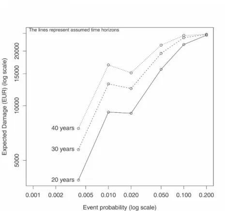
Next, we checked whether the expected monetary damage for a typical dwelling displays a similar dependency on flooding probability. It was assumed that prospective buyers may operate with time horizons of 20, 30, or 40 years in mind when discounting expected flood damage. Monetary damages per square meter for Finnish dwellings (excluding apartments) per floodwater depth group were retrieved (Mickelsson 2008, cited in Perrels et al. 2010: 65). Since these unit costs refer to floodwater depths, they were translated to indicative unit costs for different flooding probabilities, based on an assumed connection of flood frequency to floodwater depth for a given location. The unit costs were then multiplied by the average floor space of 121 m2 and by the probability of having at least one flooding event for each of the assumed time horizons, in order to produce expected flood damage costs for typical properties in the study area for the mentioned horizons.
Fig. 3 Expected flood damage for a typical dwelling in Greater Helsinki’s coast by return time
The results (plotted in Fig. 3) indicate a sharp rise in the expected damage costs as the flooding events become more probable. Notably, in the range of the F100-F50 events there is a reversal of the rising trend into a slight decrease of cost, which resembles the decrease of the estimated risk discount in Fig. 2 for the F250-F50 event range. Similarly, the two figures agree that from F10 to F5 the increase in expected damage cost and in estimated risk discount slows down. The resemblance in those two
elements becomes more pronounced as the assumed time horizon increases. The similarity between Figs. 2 and 3 renders it plausible to hypothesise that the estimated information shock is intrinsically connected to the manner in which prospective buyers assess likely damage costs over a multi-year time frame. Figs. 2 and 3 represent notably different methodologies; the former captures market response to disclosed risks, while the latter reflects calculations of technical damage costs from an engineering perspective. Their similarity serves as an additional indication that the estimated price differentials and sensitivity to flood probability are correctly identified. Furthermore, it indicates that the real estate market incorporates the extra information fairly accurately, but this is limited by biases and errors in uncertainty and risk assessment. If we compare the results at face value, the message would be that the price discounts in the market are larger than the approximated expected value of the damage, which adds to the distortion of the response to very high or very low probabilities discussed earlier. Yet, it should be emphasized that the engineering-economic calculations are rather generic, and by no means specifically meant for the considered houses. For example, other assumptions on the distribution of water depths over return times of floods can easily increase the costs, but the shape of the curve remains largely the same.
Two additional assumptions about the detected sensitivity are relevant. Firstly, the flood risk maps might have had a “confrontational” effect concerning the risk differential of otherwise similar dwellings: coastal properties exposed to frequent flooding threat re-evaluated against properties with comparable coastal amenity benefits but exposed to less a frequent threat. Secondly, buyers may react stronger to high probability or frequency than to anticipated flood water height (less frequent, but potentially with deeper floodwater). Nevertheless, more analysis is needed to sort out the behavioral aspects that underlie the discussed sensitivity, including the question of whether the economic agents have reacted in this case to flooding frequency, probability of damage, or a combination of the two.
6 Counterfactual testing
The identifying assumption of DD methodology is obviously a strong one, especially when the effects are estimated on rather volatile time series such as housing prices. Volatility may entail semi-permanent jumps in housing prices, which would be hard to distinguish from a treatment effect, and for the present estimation context this means relaxing the assumption of perfectly parallel trends between the control and treatment groups, as well as the expectation of finding a textbook DD effect. Non-stationarity is another common characteristic of housing prices, and, while not necessarily associated with volatility, this type of process can produce time series that pose similar challenges to the clear-cut expectations of DD methodology.
To rule out the possibility that the captured effects are temporal artefacts, three sets of checks were carried out. Firstly, we constructed two different control groups for the treatment group of each flood zone. In the first case, observations that fall in one flood zone but not in the next are moved from group TREAT to group CONTROL when doing estimation for the next flood zone. In the second case, instead of swapping
directly between CONTROL and TREAT, observations that are first in TREAT but out of TREAT in the next (higher frequency) zone are set aside for one step and only enter the CONTROL group in the second next step. The argument for this alternative approach is that owners may think they are still dangerously close to the zone, even though not literally in it. This is not necessarily a strictly rational behavior, but would concur with the idea that aspirant home-owners use the maps as indicative of flood risks, but do not strictly apply the numbers from the maps, or conversely they are cautious and add a margin. In both approaches of group assignment, the regressions yielded very similar results; the preceding sections report the estimations of the latter TREAT vs. CONTROL case. Secondly, we ran validation regressions in which the specifications of Tables 4a-b were repeated with a randomized year of map introduction (variable AFTERt) within the timeframe of the transactions. These test regressions returned no consistent results for the term of interest (TREATFfh * AFTERt), which suggests that the captured effect is not a random temporal artefact. In addition, the time of map introduction was different for each of the three study areas, and capturing a similar effect independently for each urban area is further indication against temporal randomness. Thirdly, high-price outliers were excluded from the sample. This, in combination with the estimation in per-square-meter units, ensures that the estimated effects reflect the majority of properties, and are not skewed by the excessive values and risk discounts of a few high-priced outliers.
Another possible interference is the financial crisis that started at the end of the previous decade, roughly at the time that the maps were published. We are confident that the financial crisis has a degree of market penetration that makes it difficult to expect that the control group would be affected differently than the treatment group in a rather homogeneous sample, when both groups are essentially the same kind of properties, mixed at the same location (flood risk areas are irregular patches of land). In other words, we have a strong case that the treatment and control groups differ only in whether they were influenced by the flood risk information or not. In addition, we have controlled for the broader macroeconomic conditions by including the regionally disaggregated unemployment rate for each study area. If the captured effect was misidentified with the effect of the financial crisis, the unemployment control should have picked that up and would have disrupted the estimations, but no such problem was present.
In summary, identifying shocks in the housing market that coincide with a broader economic depression is obviously a difficult issue for DD methodology, as is the use of volatile time series. In both cases, the limitations of the DD methodology are evident, and we caution that the inclusion of additional temporal or macroeconomic controls move beyond the original expectations or capacity of both DD and hedonic estimation.
7 Policy discussion
Urban policy and planning actions often induce shocks in the housing market, as in the case of new zoning legislation or other land use controls, transportation system modifications, local economic development decisions, or changes in environmental protection and natural hazard regulations. From a temporal perspective, the shocks can
be short-run and/or long-run effects, and while both types affect the equilibrium, the analysis of direct transaction prices—employed in this paper—measures immediate short-run shocks, whereas long-run changes are measured in the evolution of housing price appreciation indices (McCluskey 1998; McCluskey and Rausser 2000). There are indications in the PRICE/m2 and ONSALE statistics of the sample that the identified effect did not wear off in the years following the risk disclosure, but the evidence is inconclusive due to sample size and the lack of a longer time frame in the observations.
Some information about the spatial character of the policy tool can be identified by expressing Eq. 1 as a spatial regression specification. In this case, the spatially lagged transformations of the dependent and independent variables were included as right-hand variables in Eq. 1 by letting the first-order von Neumann neighborhood define the spatial weights matrix, and the resulting model was estimated in a maximum likelihood framework (Anselin 1988; LeSage and Pace 2009). The estimation and spatial impacts simulation separated the information effect into a statistically significant direct impact and statistically insignificant indirect and total impacts. Borrowing from LeSage (2008), direct impacts can be seen as effects on a typical region that are induced by a policy change in the same region, indirect are effects on a typical region induced by a policy change in neighboring regions, while total are effects on a typical region induced by a simultaneous policy change in all regions in a regional system. Thus the fact that the impacts simulation returned significant coefficients only for the direct category can be taken as an indication that the detected shock functioned as a spatially selective policy instrument in the three urban areas to which it was applied.
Combining the aforementioned temporal and spatial characteristics, it is reasonable to associate the identified information effect as a location-selective, short-run shock in the housing market. This is relevant to climate change adaptation policy as the building blocks of such policies do include information (e.g. flood maps, risk awareness) in addition to attenuation (e.g. green roofs, ‘soft areas’, elevated constructions, water resistant materials) and protection (e.g. dikes). The results suggest that measures such as the information component of an adaptation policy that are softer than more traditional tools like zoning, legislation or taxation can be as effective and can have a measurable influence on housing prices. From an urban planning point of view, such location-selective information policies can be considered as “informational zoning”. However, more elaborate spatiotemporal models have to be estimated on a longer and more populous time series than what was available for this study in order to be able to understand additional spatial and temporal details of this particular policy instrument.
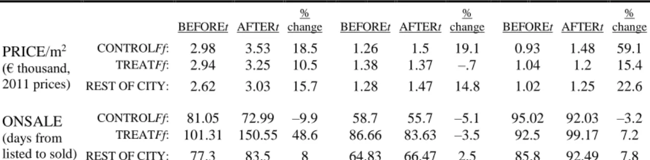
Lastly, the group comparison of variables PRICE/m2 and ONSALE of Table 2 was extended to include transactions that are unrelated to the treatment and control groups, but represent same type dwellings for the rest of the city (Table 5). The statistics show that the control group stands out in terms of decrease in the time on sale and of increase in price in the period after the map publication. Thus, the suggestion arises that the control group has benefited from a reorientation of demand from waterfront-but-risky to waterfront-but-less-risky or almost-waterfront-but-less-risky properties.
Table 5 Indications of demand re-orientation to less-risky coastal dwellings
Greater Helsinki Rovaniemi Pori
BEFOREt AFTERt
%
change BEFOREt AFTERt
%
change BEFOREt AFTERt
% change PRICE/m2 (€ thousand, 2011 prices) CONTROLFf: 2.98 3.53 18.5 1.26 1.5 19.1 0.93 1.48 59.1 TREATFf: 2.94 3.25 10.5 1.38 1.37 –.7 1.04 1.2 15.4 REST OF CITY: 2.62 3.03 15.7 1.28 1.47 14.8 1.02 1.25 22.6 ONSALE (days from listed to sold) CONTROLFf: 81.05 72.99 –9.9 58.7 55.7 –5.1 95.02 92.03 –3.2 TREATFf: 101.31 150.55 48.6 86.66 83.63 –3.5 92.5 99.17 7.2 REST OF CITY: 77.3 83.5 8 64.83 66.47 2.5 85.8 92.49 7.8
The evidence of demand re-orientation towards less risky coastal properties, the statistically significant price differential in flood-prone properties, and the fact that properties in the higher probability flood zones experienced a noticeably higher discount in comparison to those in lower probability flood zones, cumulatively suggest a correction of the spatial distribution of property values, as a result of filling-in information gaps and asymmetries. This correction is essentially a slight modification of residential location dynamics and of the resulting land value equilibrium. Since the flood-prone properties exhibit a price drop in comparison to the flood-safe properties, it can be suggested that the coastal price gradient in the flood-prone properties became shallower, moving closer to that of the flood-safe properties. This suggests that information policies about anticipated risks can affect the slope of bid-rent functions in a similar manner to realized environmental externalities (see, e.g., Brueckner 2011), whereas previous to the correction the amenity dimension of the coast was overemphasized in relation to its risk dimension. We can thus consider the information shock as a first approximation of actual flood occurrences, and utilize the estimated price discount and sensitivity to occurrence probability to simulate possible reactions of the housing market to future climate, for instance the evolution of risk perception or re-evaluation of most favorable residential areas. Furthermore, since the spatial distribution of housing prices is a key mechanism in various kinds of urban phenomena—from household and firm location equilibria to transportation and land use dynamics—the estimations can be used in urban simulations to assess how hard climate change has to kick in before we start seeing extensive and more general changes in the structure of cities than just housing price shocks.
The findings also suggest that a policy of risk disclosure for real estate markets could be extended to other forms of less obvious risk exposure, such as industrial risks or consequences of exposure to substandard air quality. As suggested above, impacts of climate change-induced changes in sea level or river run-off could be usefully illustrated in flood maps, if the changes are significant enough for markets to be picked up. An additional problem in this respect is that simulated effects of climate change usually represent cumulated effects covering, at least, several decades.
8 Conclusions
A difference-in-differences strategy was applied to detect possible housing price differentials caused by the public disclosure of high resolution flood maps in Helsinki,
Pori and Rovaniemi. The estimations have identified a statistically significant price drop, which, in the case of coastal properties in Helsinki, is sensitive to the frequency or probability of flooding. Additional controls for proximity to water aimed to separate the risk and amenity dimensions of the water body, enabling to assess more realistically the double nature of urban coastal areas. The analysis suggests that disclosure of hitherto not generally available information can be effective in addressing asymmetries and gaps concerning flood risks in the housing market. The analysis provided also indications that the real estate market processes the extra information fairly accurately. The assessment of the drivers of price response and their relative significance, at least for private home owners, does need however additional behavioral study. All in all, risk disclosure may also be relevant as a component of climate adaptation policy aimed at real estate, but in that case the gradual temporal change in the risk level poses additional communication challenges.
We propose to view the flood maps as “informational zoning” that induce a spatially selective short-run shock in the market. Lastly, we suggest that the process should not be studied only as a housing market shock, but utilized in urban economic simulations to assess modifications in the residential location and land value equilibriums under future climate.
References
Angrist, J. D., & Pischke, J.-S. (2009). Mostly Harmless Econometrics: An Empiricist’s Companion. Princeton, NJ: Princeton University Press.
Anselin, L. (1988). Spatial Econometrics: Methods and Models. Dordrecht: Kluwer Academic Publishers.
Atreya, A., Ferreira, S., & Kriesel, W. (2013). Forgetting the Flood? An Analysis of the Flood Risk Discount over Time. Land Economics, 89(4), 577–596.
Barneveld, H. J., Silander, J. T., Sane, M., & Malnes, E. (2008). Application of satellite data for improved flood forecasting and mapping. In 4th International Symposium on Flood Defence: Managing Flood Risk, Reliability and Vulnerability, Toronto, Ontario, Canada (pp. 77-1–77-8).
Bin, O., Crawford, T. W., Kruse, J. B., & Landry, C. E. (2008). Viewscapes and flood hazard: Coastal housing market response to amenities and risk. Land Economics, 84(3), 434–448.
Bin, O., Krusc, J. B., & Landry, C. E. (2008). Flood hazards, insurance rates, and amenities: Evidence from the coastal housing market. The Journal of Risk and Insurance, 75(1), 63–82.
Bin, O., & Landry, C. E. (2013). Changes in implicit flood risk premiums: Empirical evidence from the housing market. Journal of Environmental Economics and Management, 65(3), 361–376.
Bin, O., & Polasky, S. (2004). Effects of flood hazards on property values: evidence before and after Hurricane Floyd. Land Economics, 80(4), 490–500.
Brueckner, J. K. (2011). Lectures on Urban Economics. Cambridge, MA: The MIT Press.
Caldera Sánchez, A., & Andrews, D. (2011). To Move or not to Move: What Drives Residential Mobility Rates in the OECD? OECD Economics Department Working PapersNo. 846. Paris: OECD Publishing.
Card, D., & Krueger, A. B. (2000). Minimum wages and employment: a case study of the fast-food industry in New Jersey and Pennsylvania: reply. American Economic Review, 90(5), 1397–1420.
City of Pori (2009). Pori's Urban Flood 12.8.2007: Final Report (in Finnish). Conroy, S. J., & Milosch, J. L. (2011). An Estimation of the Coastal Premium for
Residential Housing Prices in San Diego County. The Journal of Real Estate Finance and Economics, 42(2), 211–228.
Daniel, V. E., Florax, R. J. G. M., & Rietveld, P. (2009). Flooding risk and housing values: An economic assessment of environmental hazard. Ecological Economics, 69(2), 355–365.
Dubin, R. A. (1988). Estimation of Regression Coefficients in the Presence of Spatially Autocorrelated Error Terms. The Review of Economics and Statistics, 70(3), 466– 474.
Dubrovin, T., Keskisarja, V., Sane, M., & Silander, J. (2007). Flood Management in Finland–introduction of a new information system. In Hydroinformatics:
Proceedings of the 7th International Conference : Volume 1 (pp. 139–146). Nice: Chennai, Research Publishing Services.
European Communities (2000). Directive 2000/60/EC of the European Parliament and of the Council of 23 October 2000 establishing a framework for Community action in the field of water policy. Official Journal of the European Communities, 43(L 327), 1–73.
Gerdes, J. (2012). What Copenhagen Can Teach Cities About Adapting To Climate Change. Forbes. http://www.forbes.com/sites/justingerdes/2012/10/31/what-copenhagen-can-teach-cities-about-adapting-to-climate-change/. Accessed 27 May 2014.
Harrison, D. M., T. Smersh, G., & Schwartz, A. L. (2001). Environmental determinants of housing prices: the impact of flood zone status. Journal of Real Estate
Research, 21(1), 3–20.
Huttunen, K., Pirttilä, J., & Uusitalo, R. (2013). The employment effects of low-wage subsidies. Journal of Public Economics, 97, 49–60.
Himanen, S. (2011). Floods and protection in Rovaniemi (presentation slides). City of Rovaniemi.
IPCC (2014). Climate Change 2014: Impacts, Adaptation, and Vulnerability. Part B: Regional Aspects. Contribution of Working Group II to the Fifth Assessment
Report of the Intergovernmental Panel on Climate Change [Barros, V.R., C.B. Field, D.J. Dokken, M.D. Mastrandrea, K.J. Mach, T.E. Bilir, M. Chatterjee, K.L. Ebi, Y.O. Estrada, R.C. Genova, B. Girma, E.S. Kissel, A.N. Levy, S.
MacCracken, P.R. Mastrandrea, and L.L. White (eds.)]. Cambridge, UK and New York: Cambridge University Press.
Kasperson, R. E., Renn, O., Slovic, P., Brown, H. S., Emel, J., Goble, R., et al. (1988). The Social Amplification of Risk: A Conceptual Framework. Risk Analysis, 8(2), 177–187.
Kahneman, D., & Tversky, A. (1979). Prospect theory: An analysis of decision under risk. Econometrica, 47(2), 263-292.
Kiel, K. A., & McClain, K. T. (1995). The Effect of an Incinerator Siting on Housing Appreciation Rates. Journal of Urban Economics, 37(3), 311–323.
Koskinen, M. (ed.) (2006). Pori’s floods – managed risks? (in Finnish), Environmental Centre of Southwest Finland, Finnish Environment no.19-2006.
Lamond, J. E. (2008). The impact of flooding on the value of residential property in the UK (PhD dissertation). University of Wolverhampton.
Lee, B., O'Brien, J., & Sivaramakrishnan, K. (2008). An analysis of financial analysts' optimism in long-term growth forecasts. Journal of Behavioral Finance, 9(3), 171–184.
Leggett, C. G., & Bockstael, N. E. (2000). Evidence of the Effects of Water Quality on Residential Land Prices. Journal of Environmental Economics and Management, 39(2), 121–144.
LeSage, J. P. (2008). An Introduction to Spatial Econometrics. Revue d’économie industrielle, 123, 19–44.
LeSage, J. P., & Pace, R. K. (2009). Introduction to Spatial Econometrics. Boca Raton, FL: Chapman & Hall/CRC.
Marttila, V., Granholm, H., Laanikari, J., Yrjölä, T., Aalto, A., Heikinheimo, P., et al. (Eds.). (2005). Finland’s National Strategy for Adaptation to Climate Change. Ministry of Agriculture and Forestry of Finland.
McCluskey, J. (1998). Environmental contamination and compensation (PhD Dissertation). University of California, Berkeley.
McCluskey, J., & Rausser, G. C. (2000). Hazardous waste sites and housing appreciation rates. CUDARE Working Papers No. 906 Department of
Agricultural & Resource Economics.Berkeley, CA; University of California, Berkeley.
Michelsson, R. (2008). Tulvavahinkojen korjauskustannukset (The repair cost of flood damages) (Master's thesis). Helsinki University of Technology.
Parjanne, A., & Huokuna, M. (Eds.) (2012). Flood preparedness in building – guide for determining the lowest building elevations in shore areas (in Finnish), Finnish Environment Institute (SYKE), Environment Guide 2014.
Peltonen, A., Haanpää, S., Lehtonen, S. (2006), EXTREFLOOD - Flood risk management in urban planning (in Finnish), The Finnish Environment report 22/2006, Ministry of the Environment, Helsinki.
Perrels, A., Veijalainen, N., Jylhä, K., Aaltonen, J., Molarius, R., Porthin, M., et al. (2010). The implications of climate change for extreme weather events and their socio-economic consequences in Finland (Vol. 158). VATT (Government Institute for Economic Research).
Pope, J. C. (2006). Limited attention, asymmetric information, and the hedonic model (PhD Dissertation). University of North Carolina.
Pope, J. C. (2008a). Buyer information and the hedonic: The impact of a seller disclosure on the implicit price for airport noise. Journal of Urban Economics, 63(2), 498–516.
Pope, J. C. (2008b). Do seller disclosures affect property values? Buyer information and the hedonic model. Land Economics, 84(4), 551–572.
Rosen, S. (1974). Hedonic Prices and Implicit Markets: Product Differentiation in Pure Competition. Journal of Political Economy, 82(1), 34–55.
Sane, M., Dubrovin, T., & Huokuna, M. (2008). A GIS-based approach for flood risk mapping - extending the national flood information system. In 4th International Symposium on Flood Defence : Managing Flood Risk, Reliability and
Vulnerability : Toronto, Ontario, Canada, May 6-8, 2008. [London, Ontario], Institute for Catastrophic Loss Reduction. London, Ontario.
Scherer, C. W., & Cho, H. (2003). A Social Network Contagion Theory of Risk Perception. Risk Analysis, 23(2), 261–267.
Sheppard, S. (1999). Chapter 41 Hedonic analysis of housing markets. In Paul Cheshire and Edwin S. Mills (Ed.), Handbook of Regional and Urban Economics (Vol. 3, pp. 1595–1635). Amsterdam: Elsevier.
Silander, J., Vehviläinen, B., Niemi, J, Arosilta, A., Dubrovin, T., Jormola, J., Keskisarja, V., Keto, A., Lepistö, A., Mäkinen, R., Ollila, M., Pajula, H., Pitkänen, H., Sammalkorpi, I., Suomalainen, M., & Veijalainen, N. (2006). Climate change adaptation for hydrology and water resources. FINADAPT Working Paper 6, Finnish Environment Institute Mimeographs 336, Helsinki.
Tversky, A., & Kahneman, D. (1973). Availability: A heuristic for judging frequency and probability. Cognitive Psychology, 5(2), 207–232.
Tversky, A., & Kahneman, D. (1974). Judgment under uncertainty: heuristics and biases. Science, 185(4157), 1124–1131.
Tversky, A., & Kahneman, D. (1986). Rational choice and the framing of decisions. The Journal of Business, 59(4), 251–278.
Votsis, A. (2014). Ecosystems and the spatial morphology of urban residential property value: a multi-scale examination in Finland. MPRA Paper No. 53742. Munich: Munich University Library.