Unique Airflow Visualization Techniques for the Design and
Validation of Above-Plenum Data Center CFD Models
by
Michael David Lloyd
B.S. Mechanical Engineering Virginia Military Institute, 2007
Submitted to the Department of Architecture in partial fulfillment of the degree of
Master of Science in Building Technology
at the
Massachusetts Institute of Technology
June 2010
ARCHNES
requirements for the
C
Massachusetts Institute of Technology 2010. All rights reserved.A u th o r ... ...
Department of Architecture May 10, 2010
Certified by ... Leon R. Glicksman
Professor of Building Technology and Mechanical Engineering Thesis Supervisor
% "-A ccep ted by ...
Julian Beinart Professor of Architecture Chair of the Department Committee on Graduate Students
Unique Airflow Visualization Techniques for the Design and
Validation of Above-Plenum Data Center CFD Models
by
Michael David Lloyd
Submitted to the Department of Architecture on May 10, 2010, in partial fulfillment of the
requirements for the degree of Master of Science in Building Technology
Abstract
One cause for the substantial amount of energy used for data center cooling is poor airflow effects such as hot-aisle to cold-aisle air recirculation. To correct these and to investigate innovative designs that will notably increase efficiency requires a robust, well-verified computational fluid dynamics
(CFD) model. Most above-plenum data center CFD models are only validated using temperature data. Although a temperature-only validation method can be useful, it does not confirm that the airflow patterns predicted by the CFD model are accurate. Since the airflow patterns above a
raised-floor plenum should be confidently understood before they can be optimized, it is necessary to adopt a validation method that offers more than just a comparison of temperature data.
This thesis summarizes the unique validation process of a CFD model for a small data center test cell located in Cambridge, Massachusetts. The validation method features point velocity and temperature measurements and the use of small neutrally-buoyant bubbles to visualize the airflow patterns above a raised-floor plenum.
The data center test cell was designed to emulate a standard hot-aisle and cold-aisle airflow configuration. The airflow visualization revealed that each perforated tile had a substantial non-uniform air velocity distribution leading to an unexpected three-dimensional flow pattern above the racks. When this surprising reality was properly accounted for in the CFD boundary conditions, good agreement was found with the observed airflow patterns. It is the purpose of this thesis to show the difficulties and value of utilizing more robust validation techniques for data center CFD models.
Thesis Supervisor: Leon R. Glicksman
Acknowledgments
This thesis, and ultimately my degree from MIT, would not have been possible without the help and collaboration of many people. I would like to generally thank everyone who was involved in the process, but a few people deserve specific recognition.
First, I must thank my academic advisor, Professor Leon Glicksman. Thank you for your guidance and support of my education and research at MIT. I learned the art of problem solving from your classes and our research meetings, and this invaluable skill will surely be one of my greatest assets in the decades to come.
Second, I must thank my mentors and friends, Matthew and Wendy Hyre. I would not be at MIT without your encouragement and help. You have already had an immeasurable impact on my life, and I cannot be more thankful for everything you have done for me.
Third, I must thank Kathleen Ross and Ali Mulcahy. You brightened my MIT experience with your friendship and help-thank you.
And last, but not least, I must thank my family. I am beyond grateful for your endless love and support.
Contents
Chapter 1: Introduction ... 11
1.1
Introduction to E nergy Issues ... 111.2 E nergy U se in Buildings... 12
1.3 E nergy U se in D ata Centers... 13
1.4 Conventional D ata Center Cooling... 14
1.5 Conventional System Issues ... 15
1.6 Com putational Fluid D ynam ics in D ata Centers ... 16
1.7 Literature R eview ... 17
1.8 M otivation and O utline of Thesis ... 23
Chapter 2: Setup of the E xperim ental Space ... 25
2.1 Introduction...25
2.2 D etails of R oom 24-032b ... 25
2.3 D etails of the Experim ental Space ... 28
2.4 D etails of E xperim ental Com puting E quipm ent ... 34
Chapter 3: Setup of the CFD M odel...38
3.1 Introduction... ... 38
3.3 G eom etry ... 40
3.4 M esh ... 43
3.5 Process...44
3.6 Post-Processing ... 58
Chapter 4: E xperim ental Results ... 59
4.1 Introduction...59
4.2 Zone 1...61
4.3 Zone 2 ... 78
4.4 Zone 3 ... 81
4.5 Server A T ... 83
Chapter 5: CFD / E xperim ental Com parison...84
5.1 Introduction...84
5.2 M odel #1 ... 87
5.3 M odel # 2...97
5.4 M odel #3 ... 106
5.5 O verall Com parison Sum m ary... 115
Chapter 6: Summary, Conclusions and Future Work ... 117
6.1 Sum m ary ... ... ... 117
6.2 Conclusions... 118
6.3 Future W ork... ... 118
List of Figures
Figure 1-1: 2008 U.S. energy value chain in quadrillion BTUs. Source (1) ... 12
Figure 1-2: 2008 U.S. primary energy consumption by sector. Source (1) ... 13
Figure 1-3: Typical data center energy end-use breakdown (PUE = 2.15). Source (3) ... 14
Figure 1-4: Conventional data center airflow configuration. Source (7)... 15
Figure 1-5: Conventional airflow configuration inefficiencies. Source (12)... 16
Figure 1-6: Overhead cooling system schematic. Source (19)...19
Figure 1-7: CFD velocity map and validation velocities. Source (19) ... 20
Figure 1-8: Data center test cell layout at IBM in Poughkeepsie, NY. Source (16) ... 21
Figure 1-9: Overall validation summary graph from paper (20) ... 22
Figure 2-1: Plan-view of the room ... 26
Figure 2-2: CRAC #1 supplied air into the raised-floor plenum ... 27
Figure 2-3: CRAC #2, which supplied air directly into the room, was ignored. ... 27
Figure 2-4: E xperim ental space... 28
Figure 2-5: Simple conventional cooling airflow design ... 28
Figure 2-6: Plan-view of the experimental space...29
Figure 2-7: T op of a perforated tile... 29
Figure 2-8: B ottom of a perforated tile...30
Figure 2-9: D esign draw ing - P 1 ... 31
Figure 2-10: A ctual picture - P 1 ... 31
Figure 2-11: D esign draw ing - P2 ... 32
Figure 2-12: A ctual picture - P2 ... 32
Figure 2-13: D esign draw ing - P3 ... 33
Figure 2-14: A ctual picture - P3 ... 33
F igure 2-15: P icture o f fan ... 34
Figure 2-16: Fan performance curve. Source (28)...35
Figure 2-17: Front-view of a server... 35
Figure 2-18: B ack-view of a server ... 35
Figure 2-19: P icture of server...36
Figure 2-20: Interior plan-view picture of a server ... 36
Figure 3-1: Flow chart for the creation of the CFD model...39
Figure 3-2: Isom etric-view of the CFD m odel...40
Figure 3-3: Isometric-view of the air-velocity inlets in the CFD model...41
Figure 3-4: Isometric-view of a server in the CFD model...42
Figure 3-5: Isometric-view of the air outlets in the CFD model ... 42
Figure 3-6: Profile-view of m eshed m odel... 43
Figure 3-7: DirectSense Air hot-wire anemometer ... 47
Figure 3-8: Velocity inlet boundary condition locations ... 47
Figure 3-9: Velocity inlet boundary condition labels ... 48
Figure 3-10: ANSYS FLUENT velocity inlet boundary condition screenshot ... 48
Figure 3-11: ANSYS FLUENT porous jump boundary condition screenshot...49
Figure 3-12: Picture of C2 calculation experiment... 50
Figure 3-13: O m ega PX 291-002W D I... 50
Figure 3-14: Cam pbell Scientific CR 1000... 51
Figure 3-15: AP vs. Velocity^2 graph of average values to show linear relationship ... 52
Figure 3-16: W att's U p Pro pow er m eter ... 53
Figure 3-17: Watt's Up Pro output graph for Server 32...54
Figure 3-18: Fan performance curve and linear fit. Source (28) ... 56
Figure 3-19: ANSYS FLUENT fan boundary condition screenshot... 56
Figure 3-20: ANSYS FLUENT outflow boundary condition screenshot...57
Figure 3-21: Boundary condition locations... 58
Figure 4-1: Sage Action, Inc. Model 5 Bubble Generator ... 59
Figure 4-2: Profile-view of data collection zones ... 60
Figure 4-3: Plan-view of inlet area jet flow region ... 62
Figure 4-4: Picture of the plenum space under the perforated tile in front of Rack 2 ... 63
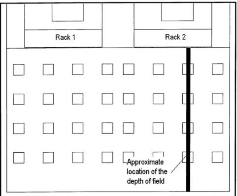
Figure 4-5: Plan-view of the approximate depth of field ... 64
Figure 4-6: Plan-view of the 14-inch data collection point locations... 65
Figure 4-7: Overview of the 14-inch point velocities and standard deviations in m/s ... 65
Figure 4-8: Velocity (m/s) vs. Time (s) line graph, at a location near point 2f...66
Figure 4-9: Picture (1) of bubbles in Zone 1, about 14 inches above the raised-floor...67
Figure 4-10: Picture (2) of bubbles in Zone 1, about 14 inches above the raised-floor...68
Figure 4-12: Plan-view of the 38-inch data collection point locations...69
Figure 4-13: Overview of the 38-inch point velocities and standard deviations in m/s ... 70
Figure 4-14: Picture (1) of bubbles in Zone 1, about 38 inches above the raised-floor...72
Figure 4-15: Picture (2) of bubbles in Zone 1, about 38 inches above the raised-floor...73
Figure 4-16: Picture (3) of bubbles in Zone 1, about 38 inches above the raised-floor...74
Figure 4-17: Plan-view of the 66-inch data collection point locations...75
Figure 4-18: Overview of the 66-inch point velocities and standard deviations in m/s ... 75
Figure 4-19: Picture (1) of bubbles in Zone 1, about 66 inches above the raised-floor...77
Figure 4-20: Picture (2) of bubbles in Zone 1, about 66 inches above the raised-floor...77
Figure 4-21: Picture (3) of bubbles in Zone 1, about 66 inches above the raised-floor...78
Figure 4-22: Front-view of jet flow region above the racks ... 79
Figure 4-23: Example of the swirl behavior noticed by the bubbles in Zone 2 ... 80
Figure 4-24: Front-view of the Zone 2 data collection point locations ... 80
Figure 4-25: Front-view of the Zone 2 data collection point velocities...81
Figure 4-26: Example of the vortices observed by the bubbles in Zone 3 ... 82
Figure 5-1: Profile-view of point locations in the CFD model...85
Figure 5-2: Another view of point locations in the CFD model ... 86
Figure 5-3: Planes used for post-processing ... 87
Figure 5-4: Profile-view of the Model #1, Zone 1 streamlines...88
Figure 5-5: Model #1 y-velocity point comparison at 14 inches in m/s ... 89
Figure 5-6: Plan-view of 14-inch plane colored by its y-velocity distribution...90
Figure 5-7: Model #1 y-velocity point comparison at 38 inches in m/s ... 91
Figure 5-8: Plan-view of 38-inch plane colored by its y-velocity distribution...91
Figure 5-9: Model #1 y-velocity point comparison at 66 inches in m/s ... 92
Figure 5-10: Plan-view of 66-inch plane colored by its y-velocity distribution...92
Figure 5-11: Model #1 x-velocity point comparison above the racks in m/s ... 93
Figure 5-12: Front-view of the plane above the racks colored by its x-velocity distribution ... 94
Figure 5-13: Profile-view of the Model #1, Zone 2 streamlines...94
Figure 5-14: Front-view of the Model #1, Zone 2 streamlines ... 95
Figure 5-15: Profile-view of the Model #1, Zone 3 streamlines...96
Figure 5-16: Model #2 velocity inlet boundary conditions...98
Figure 5-18: Model #2 y-velocity point comparison at 14 inches in m/s ... 100
Figure 5-19: Plan-view of 14-inch plane colored by its y-velocity distribution... 100
Figure 5-20: Model #2 y-velocity point comparison at 38 inches in m/s ... 101
Figure 5-21: Plan-view of plane at 38 inches colored by its y-velocity distribution... 101
Figure 5-22: Model #2 y-velocity point comparison at 66 inches in m/s ... 102
Figure 5-23: Plan-view of 66-inch plane colored by its y-velocity distribution... 102
Figure 5-24: Front-view of the Model #2, Zone 2 hand-drawn streamlines example ... 103
Figure 5-25: Front-view of an above the rack plane colored by its x-velocity distribution ... 104
Figure 5-26: Model #2 x-velocity point comparison above the racks in m/s ... 104
Figure 5-27: Profile-view of the Model #2, Zone 3 streamlines... 105
Figure 5-28: M odel #3 velocity inlet boundary conditions... 107
Figure 5-29: Model #3 y-velocity point comparison at 14 inches in m/s ... 108
Figure 5-30: Plan-view of 14-inch plane colored by its y-velocity distribution... 108
Figure 5-31: Model #3 y-velocity point comparison at 38 inches in m/s ... 109
Figure 5-32: Plan-view of 38-inch plane colored by its y-velocity distribution... 109
Figure 5-33: Model #3 y-velocity point comparison at 66 inches in m/s ... 110
Figure 5-34: Plan-view of 66-inch plane colored by its y-velocity distribution... 111
Figure 5-35: Model #3 x-velocity point comparison above the racks in m/s ... 112
Figure 5-36: Front-view of an above the rack plane colored by its x-velocity distribution ... 112
Figure 5-37: Profile-view of the Model #3, Zone 3 streamlines... 113
List of Tables
Table 1-1: Summary of published validation papers... 18Table 1-2: Summary of CFD results compared to measured data for paper (21)...23
Table 2-3: Partition w all-section m aterials... . ... 30
T able 3-4: C 2 calculation results ... 52
Table 3-5: Steady-state, averaged server power experimental measurements ... 54
Table 3-6: Summary of the CFD model boundary conditions...57 Table 4-7: Calculated bubble velocities and experimental data comparison in m/s at 14 inches.67 Table 4-8: Calculated bubble velocities and experimental data comparison in m/s at 38 inches.71
Table 4-9: Calculated bubble velocities and experimental data comparison in m/s at 66 inches.76
Table 4-10: Server inlet and outlet experimental temperature data...83
Table 5-11: Server AT comparison for CFD M odel #1 ... 96
Table 5-12: Server AT comparison for CFD Model #2... 106
Table 5-13: Server AT comparison for CFD M odel #3 ... 114
Chapter 1:
Introduction
1.1
Introduction to Energy Issues
In general, the world is careless with how it generates and uses energy. This carelessness has created numerous issues that are slowly moving from futuristic concerns to present emergencies. Ideally, people should voluntarily and thoughtfully make decisions now, instead of having to forcefully and impulsively make decisions later, about how to best deal with these energy issues.
There are a few primary energy issues that must be dealt with. First, over 90 percent of the energy currently generated in the United States has an environmentally detrimental by-product associated with its production (1). The generation of energy from oil, coal or natural gas (fossil fuels) emits carbon dioxide into the atmosphere, which is the primary culprit for global warming.
Furthermore, nuclear power plants create radioactive waste, which requires special handling and a long-term quarantine.
In addition, fossil fuels are non-renewable resources and currently used in the generation of over 80 percent of the energy consumed in United States (1). The estimated number of years left for each fossil fuel is calculated by taking the ratio of known reserves to current consumption. It is currently estimated that that for oil, natural gas and coal there are 43, 60 and 137 years left, respectively (2). The years are numbered for these non-renewable energy sources and a shift to renewable energy sources must be made.
Last, national security can be compromised because about 30 percent of the energy used in the United States is imported from other countries (1). Oil accounts for 83 percent of the energy imported to the United States and 97 percent of the energy used for the transportation sector (1).
Therefore, if a foreign government, which supplies the United States with oil, decides to stop exporting their oil, the nation's transportation system could be crippled and the country would be more vulnerable in the event of a military attack.
In order to most effectively deal with the energy issues at hand, society must improve both the supply and demand sides of the energy value chain displayed in Figure 1-1.
Figure 1-1: 2008 U.S. energy value chain in quadrillion BTUs. Source (1)
The supply side (how energy is generated) should move towards producing clean energy with local and renewable sources. The demand side (how much energy is required) should move towards
demanding less energy through more efficient use.
1.2
Energy Use in Buildings
There are three main sectors that consume energy: buildings, transportation and industrial. As shown in Figure 1-2, buildings account for 41 percent, industrial accounts for 31 percent and transportation accounts for 28 percent of the energy consumed in the United States in 2008. Therefore, buildings are the largest energy consumer in the nation and prime targets for energy
efficiency improvements.
,Pu!~m Olew E~p~r1i~
Figure 1-2: 2008 U.S. primary energy consumption by sector. Source (1)
1.3
Energy Use in Data Centers
A data center is a building or room dedicated to the continuous operation of computer servers. One report claims that data centers can consume up to 100 times the amount of energy per square foot than a typical office building (3). Unsurprisingly, the required amount of energy to operate data centers is enormous.
A 2007 EPA study estimates that data centers in the United States account for 1.5% of the nation's annual electricity consumption (4). If no action is taken to improve the energy efficiency of data centers, this amount will continue to increase as the number of servers in the United States is growing by about 10 percent each year (5).
A metric widely used to examine the efficiency of data centers is the power usage effectiveness (PUE) ratio which is the total power consumed by the facility divided by the power consumed by the servers (6). The cooling system, uninterruptible power supplies, lighting and miscellaneous loads use the power that is not being consumed by the servers. This metric is slightly misleading though because a small percentage (estimated to be at most 10 percent (3)) of the power consumed by the
servers is used to run the server fans, which are used for cooling the server. Regardless, the PUE ratio is still a useful measure for the energy efficiency of a data center.
m
Transportation
w
Buildings
a Industrial
Total Facility Power IT Equipment Power
Lawrence Berkeley National Laboratory (LBNL) initiated a benchmarking study of 22 data centers in 2001 (3). The average power allocation for the benchmarked data centers is shown in Figure 1-3. * Cooling * Servers * UPS H Lighting
aOther
Figure 1-3: Typical data center energy end-use breakdown (PUE 2.15). Source (3)
Figure 1-3 yields a PUE of about 2.15 and shows that a typical data center uses about 30 percent of its total energy for cooling. Of the data centers benchmarked in the LBNL study, the PUE range was from 1.5 to 3, which equates to a cooling energy percentage range from 11 percent to 44 percent (3). The large range of cooling energy efficiencies hints that cooling might be a great target for improving the energy efficiency of a data center.
1.4
Conventional Data Center Cooling
Most data centers are air-cooled and have their servers arranged in opposite-facing rows creating hot aisles and cold aisles. This hot aisle and cold aisle cooling approach is the most popular cooling
airflow configuration and will be called the conventional system for the remained of this thesis. In the conventional system examined by this thesis, air is conditioned by a
computer-room-air-conditioning (CRAC) unit and discharged into a raised floor plenum for distribution. Then, air exits the plenum through perforated tiles into the cold aisle. Server fans then draw the air from the cold
aisle through the servers to remove the generated heat. After the air is discharged into the hot aisle, it is pulled back to the CRAC unit to begin the cycle again. Figure 1-4 shows a cross-sectional view of this system.
Hot Aisle Hot Aisle
Cold Aisle
Return
CRAC
Supply
c-
supply air from
CRAG
to the cold
aisle
os*
distribution from cold aisle through racks
mwy
hot exhaust air return to CRAC units
Figure 1-4: Conventional data center airflow configuration. Source (7)
1.5
Conventional System Issues
The conventional system was designed in 1992 when the average power density of a rack (a rack is an open cabinet where servers are mounted) was about 1 kW (8; 3). Today, some racks consume over 30 kW (9). The conventional cooling system, though, is inherently the same despite the rapid increase in rack power densities. This has created a number of issues that researchers are currently working to understand and resolve.
Many data centers were designed for 15-20 years of use (10), but servers tend to become outdated every two years as noted by Moore's law. Cooling demand increases when servers are upgraded and eventually the cooling systems will be unable to meet the new cooling demand unless the system is upgraded or improvements are made to the airflow.
It is widely accepted that good airflow management is one of the best ways to increase the cooling efficiency of a data center. If designed properly, the conventional system can be efficient; however, this requires that some of the different system components be optimized and that some issues be avoided (11). The following list, for example, gives some ideas of the different parameters that can cause inefficiencies:
* Optimize the placement of raised-floor air discharge tiles * Optimize the pressure in raised-floor plenum
* Optimize the location of CRAC units
* Avoid recirculation of heated air over the top or around server racks * Avoid short-circuiting of cooled air back to CRAC units
* Avoid an inadequate ceiling height or undersized raised-floor plenum * Avoid air blockages in the raised-floor plenum
* Avoid openings in racks that allow air bypass from hot aisles to cold aisles
shotd-
Equpmn Recirculationa iny Racks -- A Warm air retumedt f CR AC CRAC 4RAC Hot
Venilon Tiles
is4leJ
Floor
Plenum----
Hot Air -oldRoom Chlled Water Supply
Figure 1-5: Conventional airflow configuration inefficiencies. Source (12)
ASHRAE (3), Schmidt and Iyengar (13), Greenberg et al (11) and many others have examined the system-inherent sources of inefficiencies and developed best practices to optimize airflow patterns. Airflow patterns are optimized when the supply air is directly used for cooling the servers and not short-circuited back to the CRAC unit or re-circulated from the hot aisle into the cold aisle.
Many data center researchers and operators have used computational fluid dynamics to help them understand and optimize the airflow patterns of data centers.
1.6
Computational Fluid Dynamics in Data Centers
Computational fluid dynamics (CFD) is a computational technology that can be used to study the dynamics of fluid flow and heat transfer.
The first published results of data center airflow modeling using CFD appeared in 2000 (9). Since then, CFD models have frequently been used in data center cooling analyses because the airflow in a data center is not always intuitive and tends to be highly complex (14). Data center
designers and operators can extract useful information from CFD models that can be used to optimize the airflow patterns of a data center.
However, there are some concerns about the accuracy of CFD models because the results are highly dependent on the user-inputted boundary conditions, the chosen turbulence model, definition of convergence and the level of detail in the model. Because of these concerns, it is important to validate the results of a model with experimental data.
The validation of CFD models can be an arduous process because of the complexities in
acquiring quality data from a data center environment. Because of the complex airflow patterns and difficulty in obtaining useful velocity measurements, above-plenum CFD models are typically just validated using point-wise temperature data. This is a limited approach to validation, though,
because it does not confirm that the airflow patterns (which ultimately determine the air temperatures) are correct in the CFD model.
1.7
Literature Review
Data center designers and operators frequently use CFD models to understand the airflow patterns and temperature distribution in data centers. The quality of the data obtained from CFD models is questionable, though, if the model has not been validated with experimental data. In general, there is a lack of literature on the comparisons between experimental data and CFD model predictions (15). Some papers have been published that do compare experimental data with CFD
Reference Year Published Space Modeled Validation Metric
(16) 2009 Above Plenum Temperatures
(15) 2007 Above Plenum Temperatures
(17) 2008 Above Plenum Temperatures
(18) 2009 Above Plenum Temperatures
(19) 2001 Above Plenum Temperatures*
(20) 2006 Above Plenum Temperatures
(21) 2007 Above Plenum Temperatures
(22) 2007 Above Plenum Temperatures
(23) 2004 Plenum Tile Flow Rates
(24) 2001 Plenum Tile Flow Rates
(25) 2003 Plenum Tile Flow Rates
(26) 2005 Plenum Tile Flow Rates
(27) 2007 All Tile Flow Rates
Table 1-1: Summary of published validation papers
As seen in Table 1-1, there are two metrics that researchers have used to validate CFD models: temperatures and tile flow rates. In general, the above-plenum CFD models used temperatures for validation. Conversely, the plenum-only CFD models used tile flow rate measurements for
validation. Since this thesis is only concerned with the airflow patterns above the plenum, the plenum-only studies will be ignored. Only one paper, (19), validated a CFD model beyond the normal metrics previously listed.
Patel et al. (19) published a seminal paper on data center CFD validation in 2001. It examined a prototype data center and compared experimental results with a CFD model. The prototype data center, though, had a non-conventional cooling system. The system featured a modular overhead unit that collected air from the hot aisle, conditioned the air using a heat exchanger and then released the air into the cold aisle (see Figure 1-6).
Heat Exchanger (Detail A)
Cool Fluid Hot Aisle Cold Aisle
-... Hot Fluid Cooling Coil
Fan
Unit -. Coolant, Te..ut
Coolant, Tea
A (Chilled water)
Cool Air, Tk,.t Hot Air. Ti.
Detail A. Heat Exchanger Block Diagram
Figure 1-6: Overhead cooling system schematic. Source (19)
Patel et al. validated their CFD model using both temperature and velocity measurements. Temperature data were collected at various locations and the CFD model predictions had an average error from 7 to 12 percent in the temperature readings in Celsius. In addition, velocity
measurements were used to confirm the existence of stagnation regions noticed from the CFD results. However, only five point velocity measurements were used to confirm the existence of the
stagnation regions around the racks labeled A6 and C1. The CFD velocity map with actual velocity measurements can be seen in Figure 1-7.
up n I I nWW/' Exp: +0O9 Suii: +1.0: sign- 10 =/I Exp 0.7m Ws o Sim- 03 nih jW ,S Ir i D
~
J~ oh >Lni 5 beund1c61 Stageion RegionFigure 1-7: CFD velocity map and validation velocities. Source (19)
The work of Patel et al. in this paper was much needed and appreciated by the data center CFD research community; however, the study is limited because of a few reasons. One, the paper was published in 2001 and there have been many technological advances since its release in both the data center cooling systems and the capabilities of CFD software. Two, it examined a non-conventional cooling system which provides no insight for understanding the airflow patterns of a conventional system. And, finally, although it did confirm stagnation regions using velocity measurements, velocity validation was not a primary metric for the overall validation of the model.
There are a number of published papers (18)(16) (15) (17) which have utilized experimental data collected from a data center test cell located at IBM in Poughkeepsie, New York to validate CFD models. The data center test cell has a floor area of 900 square feet and was designed to emulate a conventional cooling system; however, the layout is impractical because it does not feature cold-aisles and hot-cold-aisles, but one rack in an open room (see Figure 1-8). Furthermore, the CFD models
were validated using temperature data, which does not confirm the accuracy of the airflow patterns predicted by the CFD models.
Sypas Floor Tiles
CRAc Unk 1T Equipmet
SmitrRack
Perforatd Fkoor ies
Figure 1-8: Data center test cell layout at IBM in Poughkeepsie, NY. Source (16) For the IBM data center test cell, Cruz et al. (16) found the experimental uncertainty of their temperature readings to be about 1.8 degrees C when compared to their CFD model. Iyengar et al. (15) showed that their CFD results seemed to over-predict the hot and cold spots and under-predict the mixing between the hot and cold air streams relative to measurements. Their study resulted in an average absolute difference of 3 degrees C, and found the highest average absolute temperature difference in the region to be behind the rack. Zhang et al. (17) examined the effect that server detail has on the CFD model, airflow leakage models, and turbulence models. The increased detail in the simulated servers was found to provide no additional accuracy to the model, and the various airflow leakage models and additional turbulence models only produced a modest impact on the
temperature differences. Lastly, Cruz et al. (18) compared three cooling airflow configurations to a CFD model and yielded an overall root-mean-square difference of 3.5 degrees C with a standard deviation of 2.0 degrees C. For these studies, the approximate temperature difference between the inlet and outlet of the servers was about 10 degrees C.
Overall, the studies that utilized the IBM data center test cell in Poughkeepsie showed good agreement between the experimental and CFD temperature data. However, these studies are limited because the data center layout is impractical when compared to most data center airflow
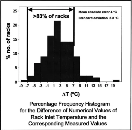
Shrivastava et al. (20) compared a CFD model to experimental data for a 130-rack conventional cooling system data center that had a floor area of 7,400 square feet, and found a mean absolute inlet air temperature error of 4.0 degrees C with a standard deviation of 3.3 degrees C (see Figure 1-9). An excellent agreement was observed in the regions of moderate rack powers and for the racks located near the CRAC units and along the aisles. The greatest differences occurred in the region of high density suggesting a need for more careful and detailed collection of data for such regions and perhaps a more detailed CFD model. Like the IBM data center test cell studies, this paper just validated the temperature distribution and not the airflow patterns.
20-6
10--9 -7 -5 -3 -1 1 3 5 7 9 11 13 15 17 19
AT ("C)
Percentage Frequency Histogram
for the Difference of Numerical Values of
Rack Inlet Temperature and the
Corresponding Measured Values
Figure 1-9: Overall validation summary graph from paper (20) Schmidt et al. (21) compared the results of a data center CFD model to experimental
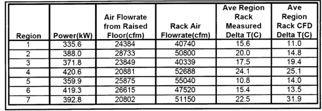
temperature data for one of the fastest supercomputers in the world. The model did a reasonable job predicting the general trends in the IT equipment inlet air temperatures, but there were some large discrepancies between the measured and predicted values. A summary of the comparison is shown in Table 1-2.
Ave Region Ave
Air Flowrate Rack Region
from Raised Rack Air Measured Rack CFD Region Power(kW) Floor(cfm) Flowrate(cfm) Delta T(C) Delta T(C)
1 335.6 24384 40740 15.6 11.0 2 388.0 28733 50800 20.0 14.8 3 371.8 23849 40339 17.5 19.4 4 420.6 20881 52688 24.1 25.1 5 359.9 25875 55040 10.8 14.0 6 419.3 26615 47520 15.4 13.5 7 392.8 20802 51150 22.5 31.9
Table 1-2: Summary of CFD results compared to measured data for paper (21)
The comparisons shown in Table 1-2 highlight some of the potential issues that are occasionally present in data centers. The total air flow rate supplied by the raised-floor plenum was insufficient to meet the demand of the racks, which mandated recirculation and lowered the efficiency of the data center. Also, this paper just validated the temperature distribution in the space and not the airflow patterns.
The published research on the validation of above-plenum CFD models is limited because they only validated the temperature distributions of the data center and not the airflow patterns.
Temperatures are important, as the ASHRAE standards are based on them (3), but the airflow patterns in the space determine the temperatures. Without an understanding of the airflow patterns, it is difficult to improve the airflow patterns.
1.8
Motivation and Outline of Thesis
There are great opportunities to increase the cooling energy efficiency of data centers. One of the primary ways to do this is to optimize the airflow patterns in the data center. In order to optimize the airflow patterns in a data center, though, the airflow patterns must be accurately understood. The current validation process for above-plenum data center CFD models does not confirm that the airflow patterns are accurate; it only confirms that the temperature distribution is accurate. As a result, the validation process must be improved. Therefore, the purpose of this thesis is to introduce unique data center validation techniques for the verification of airflow patterns in above-plenum CFD models.
The validation techniques utilize both qualitative and quantitative data. Qualitative data was acquired by the tracking and visualization of small, neutrally-buoyant bubbles in the airflow paths, and quantitative data (temperature and airspeed measurements) were collected using a hot-wire anemometer. To the author's knowledge, these techniques have never been used to validate a data center CFD model.
Chapter 2 explains the setup of the experimental space. Chapter 3 explains the setup of the CFD model. Chapter 4 shows the experimental data. Chapter 5 compares the CFD models with the experimental data. And, Chapter 6 contains the summary, conclusions and recommendations for future work.
Chapter 2:
Setup of the Experimental Space
2.1
Introduction
A
full-size, controlled experiment in an operating data center was constructed in order to gain a better understanding of the airflow patterns in a data center and to validate the CFD model. Both quantitative and qualitative analyses were performed to achieve these goals.The MIT Laboratory for Nuclear Science (LNS) operated a small data center in the basement of Building 24 at MIT. This data center was located in room 24-032b, and some space in the room was borrowed from the LNS for this experiment.
2.2
Details of Room 24-032b
The room was 688 square feet. It had a 6-inch raised-floor plenum and a ceiling height of 114 inches (9.5 feet). The raised-floor plenum did not have any notable airflow obstructions. The room
dimensions, tile layout and the approximate location of the operating computing equipment are shown in Figure 2-1.
Two c p ro i tioning FupmRdh
Figur2-3 sumpupN Eqadrlioiin
I -t i1 (. ... T- CRAG
II__
_i
#2: 14' TO-DPnk ___ L__ of 42.3 ,900 W-nd ioopeuuutilized a non-ducted return air strategy that
pulled
air into the top of the unit.CRAC #2 was ignored in this experiment because it did not influence the airflow
patterns
of the experimental space. To ensure that none of the air supplied by CRAC #2 influenced the airpatterns
in the experimental space, an air deflector was installed to divert its supply air away from theFigure 2-2: CRAC #1 supplied air into the raised-floor plenum.
2.3
Details of the Experimental Space
A space within room 24-032b was isolated for the experiment. This space (shown in Figure 2-4) was specifically designed to emulate a conventional cooling system as seen in Figure 2-5.
Figure 2-4: Experimental space
r~z>
supply air from
CRAC to the cold
aisle
tsp
distribution from cold aisle through racks
am
hot exhaust air return to CRAC units
Figure 2-6 shows a plan-view of where the experimental space was setup in the room and how the racks were oriented. The tiles were the standard size (2 ft by 2 ft). The bolded lines represent where the partitions (designated in Figure 2-6 as P1, P2 and P3) were placed.
P1
CRAC #2
Perforated Tile 1 Rack 1MOW
Perforated Rack 2 P2 Tile 2 P3 CRAC 0 18'
Figure 2-6: Plan-view of the experimental space
Perforated tiles emitted air into the experimental space. Each perforated tile had 2,842 holes and each hole had a diameter of 0.236 inches (see Figure 2-7). Therefore, the open area of each tile was 21.6 percent. However, there were structural support pieces on the back of the tiles which further reduced the actual open area to about 15 percent (see Figure 2-8).
Pigure Z-6: bottom ot a pertorated tile
Air was exhausted from the experimental space through two openings in partition P2 as seen in Figure 2-12. A window screen was put in the exhaust openings to prevent bubbles (used in the qualitative analysis) from leaving the experimental space.
The space was carefully sealed to prevent air from taking unwanted paths. For example, the partitions were placed directly adjacent to the racks to prevent airflow from going around the sides of the racks. Also, unused servers were left in the racks and their airflow openings were covered with tape, which essentially turned them into blanking panels.
The experimental space was isolated using stud-framed walls and carefully sealed. The partitions were specifically designed to allow for easy and accurate measurements and observations. The material for each section of the partitions was selected for a specific purpose. Table 2-3 explains the different materials that were used for the partitions and why they were chosen. All of the materials chosen, except for the window screen, were air-impermeable.
# Material Purpose / Comments
1 Opaque canvas, with luggage zippers To allow entry for instruments 2 Opaque felt roofing paper No visibility needed
3 Clear, hard plastic (Plexiglas) High visibility needed 4 Clear plastic shower curtain Moderate visibility needed
5 Window screen To keep bubbles from leaving the space, exhaust 6 Opaque canvas, with hook and loop fasteners Used to enter the hot-aisle and cold-aisle
25" 8" 18" 18" 8" 23' 4 4 1 3 3 3 31" 4 2 3 -113" 1 1 2 2 3 36" 100"
Figure 2-9: Design drawing - P1
26" 27" 5 5 27. EXHAUST EXHAUST 113 4 4 38" 2 2 53"
Figure 2-11: Design drawing - P2
Yigure 2-12: Actual picture - P2 SI
33" 34" 33"
113"
6
6!>I
loon
Figure 2-13: Design drawing - P3
2.4
Details of Experimental Computing Equipment
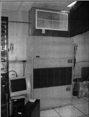
Twenty servers were used for this experiment-ten in each rack. The racks were standard Electronics Industry Association (EIA) enclosures that were 78 inches high, 24 inches wide and 30 inches deep. A standard 78-inch rack has an available height of 40U, where a U is 1.75 inches.
The experiment used VA Linux Systems servers, and each server had a height of 2U or 3.5 inches. Furthermore, each server had five 2.36-inch 12V DC axial computer fans (see Figure 2-15). The fans were manufactured by the ADDA Corporation (28) and had a model number AD0612HB-A70GL. Three fans were located across the front face of the server as seen in Figure 2-17. The other two fans (which are the same fan model as the other three) were located on the inlet and outlet of the server's power supply. The back view of the server (Figure 2-18) shows the outlet fan of the power supply, and the interior view (Figure 2-20) shows the inlet fan of the power supply. The performance curve for the fans is shown in Figure 2-16.
Figure 2-15: Picture of fan I
Fan Performance Curve
FLOWRATE(CMM) 0.000 0198 0.396 0,594 0,792 0,991 70 0-276 -6 0;22G 4,2 0.165 UU 1 4 0 0 141 0.0 0.000 0 7 14 21 28 35 FLOWRATE(CFM)Figure 2-16: Fan performance curve. Source (28)
The front of each server (Figure 2-17) had 276 holes, and each hole had a diameter of 0.157 inches. Therefore, the total open area for the front of each server was 5.38 in^2. The back of each server (Figure 2-18) had 225 holes, and the area of the fan-opening was 3.29 in^2. Therefore, the total open area for the back of each server was 7.67 in^2.
Figure 2-17: Front-view of a server
Figure z-1IV: 1icture ot server
Power Supply
Fan 4 -- Fan 5
CD-ROM >
DRIVE
Fan 1
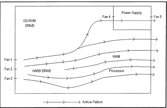
Fan 2 HARD DRIVE Processor
Fan 3
Airflow Pattern
Figure 2-21: Interior plan-view of a server with component placement and the approximate direction of airflow
Chapter 3:
Setup of the CFD Model
3.1
Introduction
For this thesis, a computational fluid dynamics (CFD) model of the experimental space was created to better understand the airflow patterns for a conventional data center cooling system. This chapter describes the setup of the CFD model.
Computational fluid dynamics is an engineering tool that is used to predict fluid flow and heat transfer phenomena by solving the mathematical equations that govern these processes using a numerical algorithm on a computer.
A CFD model was created and the results were compared with experimental data. The creation of a CFD model follows a basic procedure: process, process and post-process. During the pre-processing stage, the geometry is created. The geometry defines the physical bounds of the model. The geometry is then divided into discrete cells, which is called the mesh. After the mesh is created, the equations that model flow are selected and the boundary conditions are defined. Boundary conditions specify the fluid behavior and properties at the boundaries of the model. After the boundary conditions are set, the model is processed by iteratively solving the chosen equations. Finally, a post-processor is used for the analysis and visualization of the resulting solution.
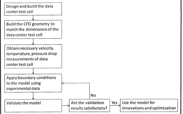
Amemiya et al. (22) published a flow chart that describes a procedure that can be used to create a data center CFD model. A similar procedure, shown in Figure 3-1, was used for the creation of this model.
Design and build the data center test cell
Build the CFD geometry to
match the dimensions of the data center test cell
Obtain necessary velocity, temperature, pressure drop measurements of data center test cell
Apply boundary conditions
to the model using experimental data
Validate the model
I
No
Are the validation Yes Use the model for
results satisfactory? innovations and optimization Figure 3-1: Flow chart for the creation of the CFD model
3.2
Software
/
Hardware
Three software programs were used in the creation of the CFD model. ANSYS Gambit 2.4.6 was for pre-processing, ANSYS FLUENT 12.0.16 was used for processing, and both ANSYS FLUENT 12.0.16 and CEI Ensight CFD 2.0 were used for post-processing.
ANSYS Gambit 2.4.6 and ANSYS FLUENT 12.0.16 were chosen to create and process the model because of their design options and flexibility. Data center specific CFD software programs are limited because they force the user to modify the model using conventional system-inherent options. Since ANSYS Gambit and FLUENT are generic CFD programs, which can be used to solve any fluid flow scenario, they offer more flexibility for the user to be innovative.
The computer used was a Dell Precision T5400 computer with an Intel Xeon CPU E5430
@
2.66 GHz and 3.25 GB of RAM. Further, the computer utilized the Microsoft Windows XP Professional x32 Edition operating system.3.3 Geometry
The first step in creating a CFD model is to create the geometry of the space to be modeled. The geometry defines the physical boundaries of the model. Since the airflow patterns above the raised-floor plenum are the primary interest of this thesis, only the space above the raised-raised-floor plenum was modeled. The boundary conditions applied to this model are explained later in this chapter.
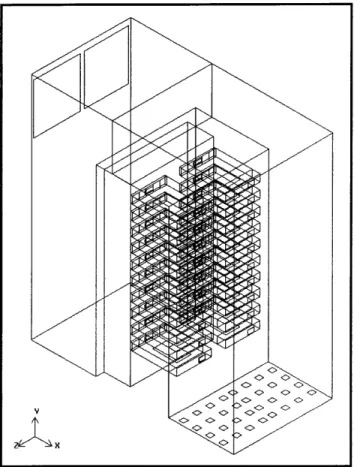
The geometry of the data center space was created using Gambit 2.4.6. An isometric view of the final model is shown in Figure 3-2. The dimensions of the room, outlets, racks and servers in the model were determined from the experimental space and equipment.
Figure 3-2: Isometric-view of the CFD model 3.3.1 Perforated Tile Geometry
If the entire face area of a perforated tile was modeled and assigned a uniform velocity, the flow rate would be accurate, but neither the velocity distribution nor the initial momentum of the flow would be properly modeled. To solve this dilemma, each perforated tile was modeled as sixteen small square velocity inlet faces. This was done so that the supply air would have the correct initial
velocity distribution and flow rate. The area of each inlet was 5.52 in^2 and the total area for sixteen smaller inlets was 86.4 in^2, which corresponds to the open area of one perforated tile.
Figure 3-3: Isometric-view of the air-velocity inlets in the CFD model 3.3.2 Server Geometry
The servers were modeled as open volumes, but each had five features: an inlet, a face to apply a pressure drop, a face to apply a heat flux, faces to apply fan conditions and an outlet.
The server pressure drop was applied to a face inside the server (see Figure 3-4) to simulate the pressure drop through the component-packed server. The server inlet area was 5.38 in^2, which corresponds to the actual open area of the front of each server. Although most data center CFD models assume a fixed flow rate for each server, this model simulated the fans by applying a fan pressure-velocity relationship to five faces located along the back of the server (see Figure 3-4). These fan faces were in series with the pressure drop face. The server outlet area was 7.67 in^2, which corresponds to the actual open area of the back of each server. Furthermore, to simulate the
heat generated by the server components, a heat flux was applied to a face at the bottom of each server as shown in Figure 3-4.
Figure 3-4: Isometric-view of a server in the CFD model 3.3.3 Outlet Geometry
The air exhaust outlet areas in the CFD model (see Figure 3-5) correspond to the air exhaust outlet areas of the experimental space (see Figure 2-12).
x--
-x ~x
-
K
3.4
Mesh
In order to examine a geometry using computational fluid dynamics, the geometry must be meshed. A mesh is a collection of points representing the flow field, where the equations of fluid motion and heat transfer are calculated. In other words, a mesh is the result of breaking a larger volume
(geometry) into smaller volumes (cells).
ANSYS Gambit 2.4.6 was used to mesh the geometry. The final mesh size was deemed
appropriate because a model with a finer mesh produced similar results with no noteworthy change. The final mesh had 1,261,263 tetrahedral cells and 260,279 nodes. Figure 3-6 shows a profile view of the meshed model.
3.5
Process
ANSYS FLUENT 12.0.16 was used to solve the model. The specific equations used to determine the fluid flow and heat transfer were chosen and applied during this step. In order to solve these equations, boundary conditions were also applied.
3.5.1
Equations
ANSYS FLUENT solves the conservation equations for mass and momentum for all flow models. For models that involve heat transfer or turbulence, additional equations are also solved.
Conservation of Mass and Momentum Equations
The general form of the equation for conservation of mass, or continuity equation, can be written as (29),
+
V - (pu)
=0
[3.1]at
The equation for the conservation of momentum in an inertial (non-accelerating) reference frame can be written as (29),
49
_V + V[3.2]~(A
+±V -(pV) (TpVi)+P9 +PF
where Pis the static pressure, Tis the stress tensor, and
P9
and Fare the gravitational body force and external body forces, respectively.Turbulence Equations
A majority of the airflow in a data center is turbulent. The calculated Reynolds numbers in a data center, even with conservative estimates for the velocities and characteristic dimensions, are
consistently greater than 10,000. Turbulent flows are characterized by fluctuating velocity fields. These fluctuations mix transported quantities such as momentum and energy. Since these fluctuations can be of small scale and high frequency, they are too computationally expensive to simulate directly in practical engineering calculations. Instead, the instantaneous governing equations can be manipulated to remove the resolution of small scales, resulting in a modified set of equations that are computationally less intensive to solve. However, the modified equations contain additional
unknown variables, and turbulence models are needed to determine these variables in terms of known quantities.
The standard
k
- E turbulence model was originally proposed by Launder and Spalding in 1974 (30). It is the most commonly used turbulence model for predicting fluid flow in data center CFD models because of its robustness, economy, and reasonable accuracy for a wide range of turbulent flows. It will be used to account for turbulence in this CFD model.It is a semi-empirical model based on model transport equations for,
k,
the turbulence kinetic energy and, E, its dissipation rate. In the derivation of thek
-e
turbulence model, the assumption is that the flow is fully turbulent, and the effects of molecular viscosity are negligible. Furthermore, thestandard
k-
Emodel
is only valid for fully turbulent flows. The turbulence kinetic energy,k,
and its rate of dissipation, e, are obtained from the following transport equations (29),-(pk) + a(pkui)=--9 (4_ p k
+
Gk +G C o - +Sk [3.3]axi z Oxj Ork Oxj
and
(pk) +
(pkui) -
([p
+ t+
Gk + G -pe-Y
+
Sk
[3.4]
ot Oxi Ox; Oak 8xj
where Gkrepresents the generation of turbulence kinetic energy due to the mean velocity
gradients.
GbLis
the generation of turbulence kinetic energy due to buoyancy. YM represents the contribution of the fluctuating dilatation in compressible turbulence to the overall dissipation rate.Cl
t,O
2,
andCle
are constants and 1.44, 1.92 and 0.09, respectively.Ok
and 0e are theturbulent Prandtl numbers with default values of 1.0 and 1.3 for k and
E, respectively. Ok and Se
are user-defined source terms. All of the constants and user-defined source terms were left as their default values.Energy Equation
The ultimate purpose of airflow in a data center is to transfer heat. Therefore, in order to simulate heat transfer, the energy equation was turned on and written as (29),
(pE)
+
V - (6(pE
+
p))
=
V - kegVT -
hhjij
+
(efr
- v)
[3.5]
where kef is the effective conductivity ( t, where ktis the turbulent thermal
conductivity, defined according to the turbulence model being used), and Jis the diffusion flux of
species J.
3.5.2 Boundary Conditions
Boundary conditions specify the flow and thermal characteristics at the boundaries of a physical model. They are critical component of a CFD model and it is important that they are specified appropriately.
Five boundary conditions were applied to this model: inlet conditions, pressure jumps, heat fluxes, fan equations and outlet conditions. In order to apply appropriate boundary conditions, data were collected from the experimental space and used to specify the boundary conditions.
Velocity Inlet Boundary Condition
Velocity inlet boundary conditions were used to define the airflow velocity and temperature at flow inlets. The air was released normal to the surface of the inlet faces. Each perforated tile was modeled as sixteen small square velocity inlet faces. The area of each inlet was 5.52 in^2 and the total area for sixteen smaller inlets was 86.4 in^2, which corresponds to the open area of one perforated tile.
Velocity inlet data were collected from the experimental space using a hot-wire anemometer. The hot-wire anemometer used was a DirectSense Air manufactured by GrayWolf Sensing Solutions. It measured both the speed and temperature of the air. The airspeed readings had an accuracy of ± 3% reading ± 0.015 m/s, and the temperature readings had an accuracy of ±1.1'C.
Figure 3-7: DirectSense Air hot-wire anemometer
Since the perforated tiles have 5,684 individual inlet holes, it would have been extremely difficult and time-consuming to obtain an accurate airspeed reading at each hole. As a result, airspeed
readings were taken at different tile locations to best determine the tile velocity distribution. In addition, airspeed readings were taken above the tiles and used to determine the proper inlet velocities. The velocity inlets are the only boundary conditions that changed in the CFD models
examined by this thesis. Because of this, the velocity inlet boundary condition values will be specifically explained in Chapter 5.
Figure 3-9: Velocity inlet boundary condition labels
Pressure Jump Boundary Condition
This server pressure drop was applied to the CFD model as a porous jump boundary condition. A porous jump condition is used to model a space that has known pressure-drop characteristics. It assumes that there is a finite thickness,
Am,
over which the pressure change is defined as a combination of Darcy's Law and an additional inertial loss term (29),Ap=
- (0V + C2
) Am
[3.6]where Ais the laminar fluid viscosity, Clis the permeability of the medium, 02 is the
pressure-jump coefficient and V is the velocity normal to the porous face. The permeability of the medium, 1, the pressure-jump coefficient,
C
2 , and the thickness of the medium,Am,
are user-inputtedterms (see Figure 3-11).
Figure 3-11: ANSYS FLUENT porous jump boundary condition screenshot
The face permeability term was ignored, by setting
a
to be le+10 m^2, and the porous medium thickness was assumed to be 1 m. Therefore, the porous jump equation was simplified to,1
Ap =-C
22
PV
2[3.7]
where
02
was determined from an experiment. The experiment consisted of a large axial fan, a server, a differential pressure transmitter, a hot-wire anemometer and some cardboard to direct airflow.Figure 3-12: Picture of U2 calculation experiment
The large axial fan was a standard floor fan. The server was the same server that was used in the racks. The DirectSense Air hot-wire anemometer, which was used for the velocity inlet boundary condition measurements, was also used for this experiment. The differential pressure manometer was an Omega low differential pressure transmitter, model number PX291-002WDI (Figure 3-13). A Campbell Scientific CR1000 acquired the data from the differential pressure transmitter (Figure 3-14).
Figure 3-14: Campbell Scientific CR1000
The large axial fan pulled air through the turned-off server. The differential pressure transmitter was used to measure the pressure drop between the front and back of the server and the hot-wire anemometer was used to determine the velocity of the air going through the server at the front face
inlet. Once the pressure drop and velocity were known, 2 could then be calculated. The density of
Scenario DeltaP (Pa) Velocity (m/s) C2 (1/m)
Fan Speedl, -1 StDev 11.08 0.65 44
Fan Speed1, Avg 11.08 0.80 29
Fan Speed1, +1 StDev 11.08 0.94 21
Fan Speed2, -1 StDev 16.02 0.72 52
Fan Speed2, Avg 16.02 0.89 34
Fan Speed2, +1 StDev 16.02 1.06 24
Fan Speed3, -1 StDev 20.66 0.85 48
Fan Speed3, Avg 20.66 1.14 26
Fan Speed3, +1 StDev 20.66 1.44 17
C2 30
Table 3-4: C2 calculation results
1.4 1.3 1.2 4 1.1 1 IA 0.9 0.8 0 0.7 .0.6 0.5 0.4 10 12 14 16 A Pressure (Pa) 18 20 22
Heat Flux Boundary Condition
A power meter was used to determine how much heat each server at steady-state operation generated. The power meter used was a Watt's Up Pro developed by Electronic Educational Devices.
Figure 3-16: Watt's Up Pro power meter
As seen in Figure 3-17, steady-state operation was not achieved by the server until about five minutes after it was turned on. Because of this, it was important to wait until the server had reached steady-state before the server power was determined.
The averaged,
Figure 3-17: Watt's Up Pro output graph for Server 32
steady-state server power measurements in watts (W) are shown in Table 3-5.
Rack 1 Rack 2 Server 7 89 Server 16 96 Server 9 57 Server 28 62 Server 11 94 Server 29 90 Server 13 62 Server 32 60 Server 15 62 Server 35 91 Server 27 63 Server 37 62 Server 19 93 Server 39 63 Server 44 72 Server 41 63 Server 23 86 Server 43 94 Server 24 89 Server 45 91 TOTAL 767 W TOTAL 772 W