San Jose State University
SJSU ScholarWorks
Master's Projects
Master's Theses and Graduate Research
Spring 2014
Bayesian Classification Using Probabilistic
Graphical Models
Mehal Patel
San Jose State University
Follow this and additional works at:
https://scholarworks.sjsu.edu/etd_projects
Part of the
Computer Sciences Commons
This Master's Project is brought to you for free and open access by the Master's Theses and Graduate Research at SJSU ScholarWorks. It has been accepted for inclusion in Master's Projects by an authorized administrator of SJSU ScholarWorks. For more information, please contact [email protected].
Recommended Citation
Patel, Mehal, "Bayesian Classification Using Probabilistic Graphical Models" (2014).Master's Projects. 353. DOI: https://doi.org/10.31979/etd.7pra-hgks
Bayesian Classification Using Probabilistic Graphical Models
A Project Presented to
The Faculty of the Department of Computer Science San Jose State University
-
In Partial Fulfillment
of the Requirements for the Degree Master of Science by Mehal Patel May 2014
2 © 2014 Mehal Patel ALL RIGHTS RESERVED
3
The Designated Project Committee Approves the Project Titled Bayesian Classification Using Probabilistic Graphical Models
by Mehal Patel
APPROVED FOR THE DEPARTMENT OF COMPUTER SCIENCE SAN JOSE STATE UNIVERSITY
May 2014
---
Dr. Sami Khuri, Department of Computer Science Date
---
Dr. Mark Stamp, Department of Computer Science Date
---
Dr. Chris Tseng, Department of Computer Science Date
APPROVED FOR THE UNIVERSITY
---
4
ABSTRACT
Bayesian Classification Using Probabilistic Graphical Models
By Mehal Patel
Bayesian Classifiers are used to classify unseen observations to one of the probable class
category (also called class labels). Classification applications have one or more features and one or more class variables. Naïve Bayes Classifier is one of the simplest classifier used in practice. Though Naïve Bayes Classifier performs well in practice (in terms of its prediction accuracy), it assumes strong independence among features given class variable.Naïve Bayes assumption may reduce prediction accuracy when two or more features are dependent given class variable. In order to improve prediction accuracy, we can relax Naïve Bayes assumption and allow dependencies among features given class variable. Capturing feature dependencies more likely improves prediction accuracy for classification applications in which two (or more) features have some correlation given class variable. The purpose of this project is to exploit these feature dependencies to improve prediction by discovering them from input data. Probabilistic Graphical Model concepts are used to learn Bayesian Classifiers effectively and efficiently.
5
ACKNOWLEDGEMENTS
I take this opportunity to express my sincere gratitude to my project advisor, Dr. Sami Khuri for his guidance, support and constant encouragement throughout this project. The project has helped me improve my technical skills. I would like to thank my committee members, Dr. Mark Stamp and Dr. Chris Tseng, for their time and effort. Finally, I would also like to thank Natalia Khuri and Dr. Fernando Lobo for their invaluable insights and suggestions.
6
TABLE OF CONTENTS
CHAPTER 1
Introduction ………. 10
CHAPTER 2 Probabilistic Graphical Models ……… 12
2.1 Introduction ……… 12
2.2 Background ……… 13
2.3 Constructing the Model ..………..………. 16
2.4 Inference using the Model ……….………. 22
CHAPTER 3 Naïve Bayes Classifier ………. 23
3.1 Model for Naïve Bayes Classifier ………..……… 23
3.2 Learning in Naïve Bayes Classifier ……….. 25
3.3 Inference in Naïve Bayes Classifier ………. 26
3.4 Advantages ……….. 27
3.5 Disadvantages ………... 28
CHAPTER 4 Entropy and Mutual Information ………. 30
4.1 Introduction ……… 30
7
4.3 Mutual Information ………. 32
CHAPTER 5 Limited Dependence Classifier ……… 34
5.1 Motivation ……… 34
5.2 Algorithm ……….. 35
5.3 Constructing Model for Limited Dependence Classifier ……….……….. 36
5.4 Inference in Limited Dependence Classifier ……… 37
5.5 Advantages ……… 38 5.6 Disadvantages ……… 38 CHAPTER 6 Implementation ……….……….. 40 6.1 Functionalities ……… 40 CHAPTER 7 Datasets and Results ………. 48
7.1 Datasets ……….. 48
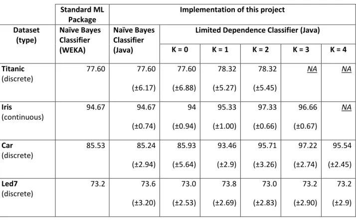
7.2 Benchmark Results ………….………. 53
7.3 Analysis ……….. 55
7.4 Summary and Future work ……… 59
8
LIST OF FIGURES
Figure 1
Joint probability distribution for student example……….
15
Figure 2
Probabilistic Graphical Model for extended-student-example…..………..
18
Figure 3
Probabilistic Graphical Model for Naïve Bayes Classifier………
25
Figure 4
Algorithm to find additional dependencies………
35
Figure 5
Header part of an example arff file……….
41
Figure 6
Data part of an example arff file………
42
Figure 7
Flow chart diagram for functionalities provided by implementation……….
46
9
LIST OF TABLES
10
CHAPTER 1
Introduction
Classification is a problem in which the end goal is to classify unseen observations to one of the class category. Classification systems (applications) have one or more features (or attributes). An observation includes a particular assignment to each of these features. A feature, separate from all other features is called as class variable and contains one or more categories. An observation can only belong to one of these class categories. A computer program which classifies Electronic-mails to one of the two categories – spam or not-spam – is an example of classification system. This system may contain a set of features such as email-sender, email-domain and number-of-recipients. An unseen observation with some value assigned to each feature could lend itself to either spam or not-spam class category.
There are several approaches to classification including probabilistic approach. Naïve Bayes Classifier is one of the widely used classifier in practice and it is based on the probabilistic approach. Naïve Bayes Classifier attempts to classify new observations to one of the class category based on the prior knowledge (known in terms of probabilities) about classification system. It uses Bayes theorem and makes strong assumption about features being independent of one another given class variable. In the case of Electronic-mail Classification example, Naïve Bayes assumption would mean that once we know about an email being a spam-email (class variable), knowledge about email-sender does not provide any additional information which is relevant towards learning more about the email-domain. Though Naïve Bayes assumption may not hold true for every application, it makes this strong independence
assumption for the purpose of classification. Naïve Bayes Classifier has good classification accuracy for the systems in which features are independent given class variable compared to for the systems in which features are strongly (or at least loosely) correlated given class variable. Dependencies among features reduce classification accuracy.
11
A better approach – Limited Dependence Bayesian Classifier [2] - is to consider additional dependencies among features while classifying unseen observations. This project aims at exploiting these additional feature dependencies to improve classification accuracy and to compare results with Naïve Bayes Classifier. We use Naïve Bayes Classifier accuracy as benchmark. Both algorithms, Naïve Bayes Classifier and Limited Dependence Classifier are implemented in Java. They were tested on classification datasets with independent features given class variable and datasets with dependent features given class variable.
The rest of this work is organized in the following fashion. Chapter 2 introduces Probabilistic Graphical Models, a framework which combines uncertainty and complexity to compactly represent high dimensional probability distributions of complex systems. In chapter 3, we discuss Naïve Bayes Classifier, a simple probabilistic classifier. Chapter 4 introduces the concepts of Entropy and Mutual Information. In chapter 5, we discuss Limited Dependence Bayesian Classifier which builds Probabilistic Graphical Models by using the concepts explained in Chapter 4. Chapter 6 focuses on the
implementation details of the Naïve Bayes and the Limited Dependence Classifier. Lastly, in chapter 7, we look at various datasets and results to compare and contrast the Naïve Bayes and the Limited Dependence Bayesian Classifier.
12
CHAPTER 2
Probabilistic Graphical Models
2.1 Introduction
Probabilistic Graphical Model is a framework which deals with uncertainty and complexity (using probability theory and graph theory) of a complex system. We construct Probabilistic Graphical Model (or just Model) for a system for which we would like to reason about what might be true under uncertainty (using probability theory), possibly given observation for various parts of the system and prior knowledge about the system. Probabilistic Graphical Model reduces complexity of any complex system by considering dependencies and independencies among various parts of the system (called features). These dependencies are shown by directed or undirected graph structure. Probability theory takes these dependencies and independencies into consideration during Model construction, inference and learning. We will see later how exploiting independencies makes our Model modular where different independent parts of the system interact using the theory of probability.
Probabilistic Graphical Model is widely used in systems where we want to answer questions with more than one possible answer (or outcome). This is possible with a Probabilistic Graphical Model due to its ability to deal with uncertainty and complexity in a manageable manner. Diagnostic Systems, Information Extraction, Computer Vision, Speech Recognition and Classification are but a few
applications (or systems) where they are used extensively. Speech Recognition systems need to output one word for a given input, assuming that the given input was a single spoken word. Humans are good at dealing with uncertainty. They use their prior experience and/or knowledge about a system for which they are asked to reason. Prior experience and/or knowledge helps them void many possible outcomes but one, which has a high degree of certainty (or belief) compared to other outcomes. For example, a person can figure out a partially heard word based on the construction and overall meaning conveyed
13
by the sentence spoken by another person. Humans take similar approaches to make inference in other domains. Computer systems can replace the need of human (expert) if we enable computer systems to take similar approaches to infer and to reach conclusions. Probabilistic Graphical Model is a framework which attempts to generalize this approach which requires prior knowledge and/or experience about a system (i.e. learning about the system).
Bayesian Classification methods are based on the fundamental principles of Probabilistic Graphical Model. The attempt at classifying given observation to one of the class category uses
Probabilistic Graphical Model constructed and trained from input data. Such classification systems have one or more features and their interaction is captured in a graph by considering dependencies (or independencies) present among these features. A graph also serves as user interface for application users. These inter-related features (except class variable) contribute towards reasoning (in our case, classification) task handled by probability theory. These two aspects deal with uncertainty and complexity of the system under consideration.
2.2 Background
Features: Systems often have various aspects which contribute towards reasoning (in our case, classification) task. These individual aspects take different values, either discrete or continuous. In the case of Electronic-mail Classification example, number-of-recipients might take continuous integer values ranging from 1 to 1000. Number-of-recipients is one aspect for Electronic-mail Classification application. Other aspects such as email-sender and email-domain take one or more discrete or continuous values. As mentioned earlier, class variable is also considered as an aspect of the given system but is considered entirely different from other aspects or features of the system.
14
The Probabilistic Graphical Model uses probability theory to attach probability to each class category and helps in determining their likelihood during inference. We first look at some important fundamentals of probability theory before we see how uncertainty and complexity are handled by Probabilistic Graphical Models.
Probability: Probability of an outcome defines the degree of confidence with which it might occur. The degree of confidence can come from belief about the possibility with which an outcome occurs and might be based on our prior experience and/or knowledge about the outcome and/or the environment in which they occur.
Probability Distribution: Probability distribution over a set of outcomes assigns likelihood to each outcome. Probability distribution for set of outcomes should sum to 1.
Conditional Probability: Theory of conditional probability defines probability distribution over an outcome α which is observed only after another outcome β occurs. It gives us likelihood of outcome α given that we already have observed outcome β. This can be represented as,
P(α | β) = P(α & β) / P(β) 2.1
Chain Rule of Conditional Probability: From eq. 2.1 we can see that P(α & β) = P(β) * P(α | β). This is known as the chain rule of conditional probability where we derive explicit joint probability distribution over all outcomes (α and β) by combining several conditional probability distributions over a smaller space. In other words, explicit joint probability distribution over all outcomes is equivalent to the probability of the first outcome multiplied by the probability of the second outcome given first outcome multiplied by the probability of the third outcome given first and second outcome and so on.
Bayes’ Rule: Rewriting eq. 2.1 we get, P(β | α) * P(α) = P(α | β) * P(β). We can derive inverse probabilities using Bayes’ rule [3]. See eq. 2.2.
15
P(β | α) = (P(α | β) * P(β)) / P(α) 2.2
Eq. 2.2 can be interpreted as follows: If we know the probability of α given β, the prior probability of β and the prior probability of α (marginal probabilities), we can derive the inverse probability – probability of β given the probability of α.
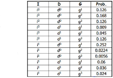
Joint Probability Distribution: Let us consider the student-example shown in Figure 1 [1]. The given system contains three features: Intelligence (I) of a student, Difficulty (D)of a course and Grade (G) of a student. Intelligence and Difficulty take two discrete values (i0 & i1 and d0 & d1 respectively for low &
high intelligence and easy & hard class) while Grade takes three values (g1, g2 and g3 for Grade A, B and
C, respectively). The joint probability distribution for this example has 12 possible combinations. This joint probability distribution can be calculated using the chain rule of conditional probability (eq. 2.1). Figure 1 specifies the explicit joint probability distribution.
16
As stated earlier, all features (except for class variable) of the given system contribute towards inference task. Inference uses theory of conditional probability to classify given observation with some value assigned to each feature. Since Probabilistic Graphical Model is based on the principles of probability theory, joint probability space over all these features is required to be calculated. Joint probability distribution over some set of features represents their joint product over all possible combinations for the values they take and assigns probability value to each. One such simple inference query we may ask here is the probability of a Highly Intelligent (i1) student getting Grade A (g1) in a Hard (d1) class, referred to as P(I = i1, D = d1, G = g1). This probability can be calculated by first using the chain rule of conditional probability to construct joint probability distribution followed by looking up the combination {i1, d1, g1}. We can see that even for such simple inference query we first have to determine explicit joint probability distribution before we can derive probability. As the number of features and their values increase, determining explicit joint probability distribution becomes quite complex and expensive. Next, we see how we reduce the complexity associated with constructing a joint probability distribution (Model) as well as how we use this Model effectively for inference.
2.3 Constructing the Model
Independent Parameters: The number of independent parameters for any explicit joint probability distribution is one less than the total number of possible combinations of that joint probability distribution. The number of independent parameters is an important property which affects the complexity of the results obtained with Probabilistic Graphical Models. For the student example, the total number of independent parameters is 11 (value of 12th parameter is determined by summing over 11 independent parameters).
17
Fewer number of independent parameters guarantees efficient computational complexity. Since inference task requires constructing joint probability space, it is convenient to have fewer independent parameters. As an example, consider a system with N features each taking two discrete values. The joint probability distribution in this case has (2N – 1) independent parameters. Because of its exponential space, larger N would require large number of independent parameters. Exponential runtime complexity is bad for computation. A system with just 20 binary discrete features will require 1,048,575
independent parameters to obtain joint probability space.
Computing joint probability distribution over exponential number of independent parameters already seems impractical. Probabilistic Graphical Model provides a framework which encodes such complex and costly to compute high-dimensional probability distribution in a compact manner. Here, we exploit independencies present among features to reduce the complexity and describe them compactly using Probabilistic Graphical Model. This Model can then be used effectively for learning and inference. 2.3.1 Dealing with Complexity
Probabilistic Graphical Model uses graph representation (directed or un-directed) to compactly represent a joint probability space which often gets complex with increased computational complexity as number of features increase. Fewer features, each with large number of values also contribute towards increased complexity and computational cost.
A graph has a set of nodes and edges. Nodes in a graph correspond to features while arcs represent interaction between pair of nodes (dependency). Lack of arc between pair of nodes represents no interaction or dependence. A graph can be a directed graph (Bayesian Network) or an undirected graph (Markov Networks). Classification applications often use directed graphs.
18
Let us consider extended-student-example of Figure 2 [1] which adds two more features to earlier mentioned student-example of Figure 1. We borrow Intelligence, Grade and Difficulty from student-example and add two more features, SAT Score (S) of a student and Letter of Recommendation (L) that students get from class teacher. SAT Score takes two values (s0 & s1 for low and high SAT score) and Letter of Recommendation takes two values (l0 & l1 for low and high quality of Letter of
Recommendation). If we assume certain independencies among these features, we can represent Probabilistic Graphical Model for extended-student-example as shown in Figure 2.
Figure 2 Probabilistic Graphical Model for extended-student-example [1]
Upon careful observation, we note that not every pair of features is connected (probabilistic independence). Difficulty and Intelligence does not depend on any other feature while Grade depends only on Intelligence and Difficulty, SAT score depends only on Intelligence and Letter of
recommendation depends only on Grade.
If we were to consider full dependencies among these features, every feature would have an arc to every other feature (without loops). This means that the explicit joint probability distribution would still require maximum possible number of independent parameters (one less than the total possible combinations). But, by considering independencies we remove unwanted arcs (interactions) between certain pair of features which reduces the complexity associated with constructing joint probability
19
distribution. Let us first construct explicit joint probability distribution for extended-student-example with full feature dependencies using the chain rule of conditional probability (eq. 2.1) as shown in eq. 2.3.
P(D, I, G, S, L) = P(D) * P(I |D) * P(G | I, D) * P(S | G, I, D) * P(L | S, G, I, D) 2.3 Here, the joint probability distribution with full feature dependencies requires 47 independent
parameters as it has 48 entries (2*2*2*2*3 = 48, each feature except Grade takes two discrete values and Grade takes 3 discrete values). However, by capturing independencies we reduce the total number of independent parameters to 15. Here is how: We have five probability distributions (referred to as factors) which if multiplied together will generate the same probability distribution as that of explicit joint probability distribution. Based on above assumed independencies, these five factors are: P(I), P(D), P(G | I, D), P(S | I) and P(L | G). The first two factors P(I) and P(D) are binomial probability distributions and require one independent parameter. Third factor P(G | I, D) has four multinomial distributions over S and I. This requires two independent parameters for each multinomial distribution. The Fourth factor P(S | I) has two binomial probability distributions over two values of I. Each of these requires one
independent parameter. The last factor P(L | G) has three binomial distributions over three values of G with one independent parameter for each binomial distribution. This gives us a total number of independent parameters equal to 15.
Factor is a function, which takes one or more features as arguments and returns a value of every possible combination for values that supplied features take. Formally, “a Factor φ (X1,X2...,Xn) is a
function where φ : Value (x1,x2...,xn) φ R and scope = {X1,X2...,Xn}” [1]. (For the rest of the
discussion features are represented using ‘upper case’ English letter while their values are represented using ‘lower case’ English letter.)
20
Any inference query can now be answered using these individual factors where each factor encodes dependencies only among features they care about. Interaction among these factors is handled by joint probability distribution of these factors. Joint probability distribution for extended-student-example can now be rewritten as:
P(D, I, G, S, L) = P(D) * P(I) * P(G | I, D) * P(S | I) * P(L | G) 2.4 Eq. 2.4 is called chain rule for Bayesian Network. If we compare chain rule for Bayesian
Network with chain rule of conditional probability (eq. 2.3), we can see that conditional independence removes unwanted feature independencies from probability distribution. Consider an example where we assume that SAT Score depends only on students’ Intelligence. According to conditional
independence if (X
⊥
Y | Z) then P(X | Z, Y) = P(X |Z). Applying conditional independence of type (S⊥
G, D | I) to P(S | I, G, D), we get P(S | I, G, D) = P(S | I). Similarly we can reduce P(I |D), P(G | I, D) and P(L | S, G, I, D) to P(I), P(G | I, D) and P(L |G) respectively. This gives us joint distribution similar to eq. 2.4.This small example showed us how conditional independence can construct explicit joint probability distribution with fewer independent parameters. More generally, any system with N binary features, where each feature has at most K parents (dependencies) has N*2k independent parameters [1] as opposed to 2N – 1 independent parameters for explicit joint probability distribution. As N increases, reduction in number of independent parameters make significant difference in obtaining compact representation of resulting Probabilistic Graphical Model. A joint probability of all features taking some value can now be calculated by multiplying probabilities from required factors where each factor has conditional probability distribution for group of features. P(G = g1, D = d1, I = i1) can now be
21
calculated using three factors P(I), P(D) and P(G | I, D) which omits the need of constructing the explicit joint probability distribution. Much more complex inference queries can also be answered efficiently using this compact form of joint probability distribution.
Graph in Probabilistic Graphical Model is perceived from two different perspectives:
Perspective 1 (What it shows): “A graph represents set of independencies that holds in a distribution” [1].
Given a graph representing a complex probability distribution space, we can read
independencies from the graph that underlying probability distribution holds. These independencies are conditional independencies where one feature is independent of all other features except their
descendents given its parents. They are represented as (X ⊥ Y | Z). Extended-student-example had several such conditional independencies. We assumed that SAT Score (S) is independent of all other features if we have evidence about Intelligence (I). This conveys that if we already know Student’s Intelligence, Difficulty and/or Grade does not provide any additional information to reason about student’s SAT Score.
Perspective - 2 (Reason we use it) – “A graph is a data structure which compactly represents high-dimensional probability distribution.”*1+
On the other hand, a graph is a data structure which encodes high-dimensional probability distribution in a compact manner, using smaller size factors. Exploiting conditional independence reduces the number of independent parameters by breaking down the distribution into a number of factors where each factor has a subset of features. Each factor’s joint probability space is much smaller as compared to the joint space of explicit joint probability distribution.
22
Bayesian Classifiers benefits from the fact that exploiting conditional independence among features gives us a compact Model. Compact Model helps with effective inference and Model learning. 2.3.2 Dealing with Uncertainty
The second aspect of Probabilistic Graphical Model deals with uncertainty. Real world
applications often have more than one possible outcome for given set of inputs. Classification systems often contain at least two or more class categories to which we wish to classify set of unseen
observations. We consider all possible class categories during classification and attach a probability to each of them to determine their likelihood with respect to given set of observed inputs.
2.4 Inference using the Model
The kind of questions we are interested in asking from a Probabilistic Graphical Model constructed for classification systems are answered based on the theory of conditional probability. A system for Electronic-mail classification takes as input email address of email-sender,
number-of-recipients and email-domain of the email-sender. Together, all three inputs become our observation and we try to question as follows: “Given an observation about email-sender, email-domain and number-of-recipients; what is the probability of email being spam?” Here, we use the chain rule for Bayesian Network (eq. 2.4) and Bayes’ theorem (eq. 2.2) to derive probability values. More detailed explanation is given in subsequent chapters.
We decide one class category based on some criteria after we compute the posterior probability of each class category (i.e. spam & not-spam). We use Maximum a Posteriori estimation technique to pick the most probable class category among all categories (to be covered in chapter 3).
In the following chapter, we study how to construct, learn and infer from Probabilistic Graphical Models for Naïve Bayes Classifier.
23
CHAPTER 3
Naïve Bayes Classifier
3.1 Model for Naïve Bayes Classifier
Naïve Bayes Classifier is considered as a restrictive classifier as it does not allow any feature dependencies given class variable. This project focuses on classification problems involving only one class variable.
If two features are independent, learning about one feature doesn’t affect the belief about other. Two features are considered independent if their joint probability distribution satisfies conditions given by eq. 3.1.
P(α, β) = P(α) * P(β)
P(α | β) = P(α) 3.1
Similarly, we define conditional independence where two features become independent given the third feature. Earlier we saw that (S
⊥
G | I),where SAT Score and Grade each depends on student’s Intelligence. Knowing about SAT Score does not add any new information to what we already have gathered about Grade after knowing Intelligence. More generally, conditional independence should satisfy condition of eq. 3.2.P(α | β, γ) = P(α | β), where (α
⊥
γ | β) 3.2 In Naïve Bayes Classifier, all features are assumed to be independent of one another given class variable. If the given system has N features X1, X2, X3…XN and class variable C, conditional independence24
For i, j in 1…N, (Xi
⊥
Xj | C), i!=j 3.3In the presence of strong independence assumption, each feature (Xi’s) contributes
independently towards the probability of some observation falling into one of the class category. Probabilistic Graphical Model for Naïve Bayes Classifier can now be constructed by considering conditional independencies of eq. 3.3. We start with explicit joint probability distribution and convert it to Probabilistic Graphical Model as shown next.
Explicit joint probability distribution for X1, X2, X3…XN and class variable C can be written as
follows using the chain rule of conditional probability.
P(C, X1, X2, X3…XN) = P(C) * P(X1 | C) * P(X2 |C, X1) * P(X3 | C, X1, X2) ... * P(XN |C, X1, X2, X3
…
XN-1)3.4 If we consider conditional independencies of eq. 3.3, probability distribution of the form P(XN | C, X1, X2, X3…XN) reduces to P(XN | C) since XN is considered independent of all other features
given class variable. Applying this reduction on all applicable factors in eq. 3.4 gives us the following compact form of the joint probability distribution where we have N factors for each feature and one marginal distribution for class variable.
P(C, X1, X2, X3…XN) = P(C) * P(X1 | C) * P(X2 |C) * P(X3 | C) * P(X4 | C) ... * P(XN|C)
= P(C) * ∏ P(Xi | C), 1 ≤ i ≤ N 3.5
The above Probabilistic Model can be encoded using Directed Acyclic Graph (Bayesian Network) as shown in Figure 3 [1]. Each feature is only dependent on one other feature – class variable.
25
Figure 3 Probabilistic Graphical Model for Naïve Bayes Classifier [1]
This new compact Model with conditional independence significantly reduces the total number of independent parameters. This compact representation is less expressive compared to the explicit joint probability distribution as we consider features to be independent of one another given class variable.
We also get modular architecture by exploiting conditional independence [1]. Probabilistic Graphical Model allows addition of new features without significant changes to existing Model. Suppose we wish to add an N+1th feature to some existing Model with N features and class variable C. We only need to add one additional factor, P(XN+1 | C) to construct the expanded joint probability distribution.
This does not require any changes to the other factors already constructed in eq. 3.5. On the other hand, the addition of one or more features in the explicit joint probability distribution requires re-writing of the entire joint distribution.
3.2 Learning in Naïve Bayes Classifier
Learning with respect to Classification corresponds to known structure and complete Data [1]. Known structure refers to known dependencies (or independencies) present in the given system. Complete data refers to the set of input data in which each observation contains some assignment to all features and class variable (with occasional missing values for some features and/or class variable). We
26
already know the structure of Probabilistic Graphical Model for Naïve Bayes Classifier as we restrict feature dependencies given class variable, which gives us Model structure shown in Figure 3 (or eq. 3.5).
Once the Model is constructed, we learn the Model from input data. Model learning populates conditional probability distribution of each factor. For Naïve Bayes Classifier, probabilities in all factors P(Xi |C) and marginal distribution P(C) for class variable C are populated using input data (training data).
3.3 Inference in Naïve Bayes Classifier
Since our goal is to classify unseen observations to one of the class category, we use
Probabilistic Graphical Model learned from training data. As explained earlier, Naïve Bayes assumption indicates that each feature contributes independently when classifying observations to one of the class category. This indicates that we compute posterior probability of each feature individually since their interaction is restricted. We use Bayes’ theorem (eq. 2.2) to compute posterior probability for each feature. P(C = c | X1 = x1) = {P(C = c) * P(X1 = x1 | C = c)} / P(X1 = x1) P(C = c | X2 = x2) = {P(C = c) * P(X2 = x2 | C = c)} / P(X2 = x2) P(C = c | X3 = x3) = {P(C = c) * P(X3 = x3 | C = c)} / P(X3 = x3) ……. P(C = c | XN = xn) = {P(C = c) * P(XN = xn | C = c)} / P(XN = xn)
In order to obtain posterior probability for (C = c), we multiply the above computed posterior probabilities. Similarly, we compute posterior probability for each class category {c1, c2, c3 … cn}.
However, this approach is not correct since observations contain all features (we do not consider class variable) and we need to consider all these features at the same time during classification even though
27
they are considered independent given class variable. We use eq. 3.5 and extended form of Bayes’ theorem as we shall now see.
The extended form of Bayes’ theorem is given by:
P(C | X1, X2, X3 … XN) = P(C, X1, X2, X3 … XN) / P(X1, X2, X3 … XN) 3.6
From eq. 3.5 we have,
P(C, X1, X2, X3…XN) = P(C) * P(X1 | C) * P(X2 |C) * P(X3 | C) * P(X4 | C) ... * P(XN|C) 3.7
Using eq. 3.7 in 3.6 we get,
P(C | X1, X2, X3 … XN) = P(C) * P(X1 | C) * P(X2 |C) * P(X3 | C) * P(X4 | C) ... * P(XN|C) / P(X1, X2, X3 … XN)
3.8 Eq. 3.8 gives us the posterior probability for class variable which considers all features of an observation at the same time. We compute posterior probability for each class category using eq. 3.8.
Classification Result = argMaxC P(C | X1, X2, X3 … XN) 3.9
where argMaxC = Maximum a Posteriori
Decision rule of eq. 3.9 selects class category with maximum posterior probability by considering only the numerator term of P(C | X1, X2, X3 … XN) since the denominator (P(X1, X2, X3 … XN)) is the same
irrespective of class category. This is essentially the class category to which Naïve Bayes classifies the given observation.
3.4 Advantages
Naïve Bayes Classifier has less computing overhead due to its restrictive assumption. Each feature is bound to have only one dependency with class variable which gives us very simple
Probabilistic Graphical Model. Moreover, Naïve Bayes assumption reduces the number of independent parameters which makes learning and inference tractable and less complicated as mentioned earlier.
28
Naïve Bayes Classifier can perform quite well even with small datasets. Since we are not capturing any dependencies among features, Model can be learnt easily and efficiently from small datasets. For example, consider a system with two features A and B (and class variable C) which takes 2 and 3 discrete values, respectively. Suppose, consider that A and B is independent given class variable. In order to learn factors P(A | C) and P(B | C) in our Model, we require that A and B’s each discrete value appears in at least one observation that is classified to each class category. This is highly probable with small datasets. Now suppose that B depends on A (as well as on class variable). Our Model captures their interaction in factor P(B | A, C). P(B | A, C) is a conditional probability distribution and has all possible combinations from the joint probability space of A, B and C. However, these combinations are in a different form where for each combination from A and C’s joint probability space, one probability value is assigned to each value of B. In order to learn our Model from data, we at least need one observation for each combination from the joint probability space of A, B and C. Small datasets do not guarantee that every combination is present in the training dataset and as a result Model may not be learnt efficiently. As the number of features in a conditional probability table increases, the efficiency of Model learning decreases.
3.5 Disadvantages
Strong independence assumption in Naïve Bayes Classifier makes classification accuracy (defined in chapter 6) less accurate compared to the accuracy had there been a consideration of dependence among features (given that features are indeed dependent). Naïve Bayes Classifier sometimes over-estimates classification results. This happens because two (or more) dependent features are considered independent given class variable where each contributes independently during classification. Eq. 3.5 multiplies these probabilities which over counts probabilities from dependent
29
features and over-estimates the observation’s actual class category (which reduces resulting probability value). This may lead to poor classification accuracy.
Naïve Bayes Classifier performs poor when the number of features increases as well as when features have dependencies. In order to improve classification accuracy for systems where features have dependencies, we need to capture their interaction in our Model. We might argue that capturing these additional dependencies may increase complexity. However, as noted before, Probabilistic Graphical Model helps manage complexity by breaking down the system into one or more independent factors.
Chapter 4 and chapter 5 investigate how we might determine additional dependencies (separate from dependencies with class variable) for classification systems and for the construction of our Model considering these dependencies.
30
CHAPTER 4
Entropy and Mutual Information
4.1 Introduction
Probabilistic Graphical Model is a framework which generalizes Model construction, learning and inference. Similarly, we need to devise an approach which can generalize discovery of additional dependencies among features to improve upon the Naïve Bayes Classifiers’ classification accuracy.
The correlation between two or more features can be determined using the concept of Entropy and Mutual Information. The concept of Mutual Information is based on the notion of Entropy. We first consider the definition of Entropy followed by Mutual Information. This becomes the basis for the discussion of chapter 5.
4.2 Entropy
“Entropy of a feature (or random variable) is a function which attempts to characterize
unpredictability of a feature”[5]. Entropy is also the measure for the amount of information that can be learned on an average from one instance of a given feature. Feature X with one bit of entropy needs on an average one bit to represent one instance. Entropy is measured in bits, nats or bans (logarithmic base 2, e and 10, respectively).
Deterministic features have zero entropy as entropy measures amount of uncertainty with which they take some value. The entropy of feature X is calculated using eq. 4.1 and is always non-negative.
H(X) = P(X) * log2 (1 / P(X)), for all values x in X 4.1
The entropy of a feature does not depend on the values it take but on the probability distribution of its values. Consider example 4.1 and 4.2 to get a better understanding of entropy.
31 Example 4.1:
Consider feature X with two discrete values {0, 1} and two observations {0, 1}. Assume that the probability distribution for X as P(X = 0) = 1/2 = 0.5 and P(X = 1) = 1/2 = 0.5. Applying eq. 4.1 we get,
H(X) = P(X = 0) * log2 (1 / P(X = 0)) + P(X = 1) * log2 (1 / P(X = 1)) = 0.5 * log2 (1 / 0.5) + 0.5 * log2 (1 / 0.5)
= 0.5 * log2 (2) + 0.5 * log2 (2) = 1 bit
The entropy of feature X is 1 bit. With 1 bit of entropy we can learn 1 bit of information about feature X. Example 4.2:
Consider feature X with one discrete value {0} and two observations {0, 0}. The probability distribution for X is P(X = 0) = 2/2 = 1. Applying eq. 4.1 we get,
H(X) = P(X = 0) * log2 (1 / P(X = 0))
= 1 * log2 (1 / 1)
= 1 * log2 1
= 0 bit
The entropy of feature X is 0 bit. Since feature X takes exactly one kind of discrete value, it is deterministic in nature. We can be certain about the value feature X takes, all the time.
Similar to the concept of conditional probability, conditional entropy measures the amount of information needed to describe feature Y given that another feature X is observed [7]. The conditional entropy of feature Y given feature X can be calculated using eq. 4.2.
32
As an example, consider two features X and Y taking the following values with the following set of observations.
Feature X: {A, B} Feature Y: {A, B}
Observations: {AA, AB, BA, BB} (in the form {XY})
In order to calculate H(Y | X) we consider all possible combinations of X and Y and apply eq. 4.2. We get, H(Y | X) = H(Y = A | X = A) + H(Y = B | X = A) + H(Y = A | X = B) + H(Y = B | X = B)
= – P(Y = A, X = A) * log2 (P(Y = A | X=A)) – P(Y = B, X = A) * log2 (P(Y = B | X = A)) –
P(Y = A, X = B) * log2 (P(Y = A | X = B)) – P(Y = B, X = B) * log2 (P(Y = B | X = B))
= – 0.25 * log2(0.5) – 0.25 * log2(0.5) – 0.25 * log2(0.5) – 0.25 * log2(0.5)
= 0.25 + 0.25 + 0.25 + 0.25 = 1 bit
We can derive one bit of information about Y (A or B) when we know the value of X. However, X and Y in this example are independent of each other and their self-entropy is also 1 bit.
4.3 Mutual Information
Using the definition of entropy and conditional entropy, we can calculate the amount of information shared between two features. I(X, Y) represents mutual information between X and Y. By definition,
I(X ; Y) = H(X) – H(X | Y) = H(X) + H (Y) – H(X, Y)
= P(X, Y) * log2(P(X, Y) / {P(X) * P(Y)}), for all values x, y in X, Y 4.4
We subtract the amount of uncertainty that remains about X after knowing Y from the amount of uncertainty about X.
Mutual information between two features X and Y is zero if they are independent. It is between 0 and 1 if X and Y are correlated. The higher the correlation the higher the value of mutual information.
33
Mutual information between two features X and Y is 1 if the knowledge about feature X can tell us exactly about feature Y or vice versa.
Consider an example with two features X and Y as below:
X takes two discrete values {A1, B1} Y takes two discrete values {A2, B2}
Observations = {A1A2, A1B2, B1A2, B1B2} (in the form {XY}) Using eq. 4.4 for all combinations of X and Y we derive I(X ; Y) = 0 bits. Since X and Y are
independent, they do not share any information. Here, probability of A1 given A2 (or B2) is the same as the probability of B1 given A2 (or B2). However, adding one more observation {A1A2}, I(X ; Y) increases to 0.019 bits. The probability with which {A1A2} and {B1A2} occurs is no more equal when we add new observation {A1A2} which increases the probability of {A1A2}. This makes the two features dependent with some correlation.
Similar to the definition of conditional entropy, conditional mutual information tells us the amount of information shared between two features X and Y given that we know feature Z. Conditional mutual information for three features X, Y and Z can be calculated using eq. 4.5.
I(X ; Y | Z) = H(X | Z) – H(X | Y, Z) 4.5
Next, in chapter 5 we study an algorithm to find feature dependencies based on the concepts discussed in this chapter.
34
CHAPTER 5
Limited Dependence Classifier
5.1 Motivation
Since the Naïve Bayes Classifier does not allow dependencies among features, it does not reflect dependencies in classification results. We thus apply the concept of mutual information to identify additional dependencies among features. We choose the best pair of dependent features based on some criteria (mentioned later) and consider them while constructing Probabilistic Graphical Model.
There are two extremes to classification applications with respect to allowable dependencies. At one extreme we have Naïve Bayes Classifier on the principles of no additional dependencies except for those among each feature and class variable. At the other end we have the General Bayesian Classifier with full degree (every possible pair is connected) of dependencies. The explicit probability distribution for General Bayesian Classifier has a class variable as a parent for every other feature. The first feature is a parent of every other feature except for the class variable. The second feature is a parent of every other feature except for the first feature and the class variable and so on. One way of selecting features as parents of other features can be based on topological ordering. There cannot be dependencies in both directions for any pair of features since a Bayesian Network is an acyclic dependency graph.
Limited Dependence Bayesian Classifier [2] discovers feature dependencies using mutual information and uses that information to construct Probabilistic Graphical Model. It limits each feature to take a maximum of K parents excluding the class variable. Parameter K can take value anywhere between two extremes (no dependence of Naïve Bayesian Network to full dependence of General Bayesian Network). Making K equal to zero gives us Naïve Bayes Classifier while making K equal to N-1 gives us the General Bayesian Classifier given that there are N features.
35 5.2 Algorithm
Figure 4 [2] shows the pseudo code for discovering additional dependencies in any system. The algorithm takes as input a dataset consisting of pre-classified observations and a parameter K and outputs Probabilistic Graphical Model. We assume that given system has N features X1, X2, X3 … XN and a
class variable C. All features are assumed to be discrete in nature (more details in chapter 6).
Figure 4 Algorithm to find additional dependencies [2] 5.2.1 Algorithm Analysis
The algorithm in Figure 4 computes the mutual information of the form I(Xi ; C) (eq. 4.4) for
each feature Xi and class variable C. It also computes conditional mutual information of the form
I(Xi ; Xj | C) (eq. 4.5) for each pair of features Xi and Xj given class variable C. Additional dependencies are
then determined considering the following fact: When classifying any observation to one of the class category, feature(s) having high mutual information (I(Xi ; C)) with class variable C more likely provides
36
(I(Xi ; C)) with class variable. Thus, the algorithm in Figure 4 (step 5.1) selects features one by one in
decreasing order of their mutual information with class variable C.
After selecting closely dependent feature with class variable in each iteration, we look at amount of information shared between the selected feature and other features given class variable (I(Xi ; Xj | C)). The higher the mutual information between the two features given class variable (eq. 4.5),
the more likely they are to have strong dependency. We select K (parameter K as explained earlier) such features among all other features for the selected feature, which has the highest value for I(Xi ; Xj | C).
Since we already have the mutual information of the form I(Xi ; Xj | C) for each pair of features (step 2),
we can determine K eligible features (Xj’s) for selected feature Xi. These set of K features and Xi more
likely provide strong evidence than the left over Xj’s (with lower mutual information with Xi) and Xi while
classifying any observation. This step is carried out in step 5.4.
The set of K new features becomes parents of the selected feature (class variable is a default parent of each feature). These steps are repeated for each Xi which gives us new dependencies for each
feature. The number of dependencies for each feature ranges from 0 to K depending upon how much or how less information they share with class variable C, respectively.
Since we give preference to features that share the most with class variable, we capture at least a few important dependencies (if any). The algorithm does not introduce any loops while adding
additional feature dependencies.
5.3 Constructing Model for Limited Dependence Classifier
We can construct Model for Limited Dependence Classifier by considering the following dependencies of eq. 5.1.
37
P(C, X1, X2, X3 … XN) = P(C) *
∏
P(Xi | Par(Xi)) 5.1where 1 ≤ i ≤ N and Par(Xi) = Parents of Xi
Learning the Model in Limited Dependence Classifier is the same as we saw with the Naïve Bayes Classifier. We have N factors of the form P(Xi | Par(Xi)), where Par(Xi) represents parents of Xi.
Depending upon the value of parameter K, each feature has 0 to K parents in addition to class variable. Unlike Naïve Bayes Classifiers’ Probabilistic Graphical Model, Limited Dependence Classifier has different Probabilistic Graphical Model for each classification system.
5.4 Inference in Limited Dependence Classifier
Classifying an observation from learnt Model involves computing posterior probability for each class category as we saw with the Naïve Bayes Classifier. We use the following equation to calculate the posterior probability.
P(C | X1, X2, X3…XN) = P(C, X1, X2, X3…XN) / P(X1, X2, X3 … XN) 5.2
Using eq. 5.1 in eq. 5.2 we get,
P(C | X1, X2, X3…XN) = P(C) *
∏
P(Xi | Par(Xi)) / P(X1, X2, X3 … XN), 1 ≤ i ≤ N 5.3Applying eq. 5.3 to each class category and neglecting the term in the denominator (it is same irrespective of class category) we get the most probable class category using the following criteria (same as eq. 3.9):
Classification Result = argMaxC P(C | X1, X2, X3 … XN) 5.4
where argMaxC = Maximum a Posteriori
Similar to the Naïve Bayes Classifier, Limited Dependence Classifier also reduces the number of independent parameters. However, the number of independent parameters increases with the value of parameter K. For K = N-1 (including class variable), the number of independent parameters becomes
38
equal to the number of independent parameters of explicit joint probability distribution (since each possible pair is connected).
5.5 Advantages
Limited Dependence Classifier improves the classification accuracy for systems with dependent features. If the features are indeed independent, the accuracy of Limited Dependence Classifier falls back to that of the Naïve Bayes Classifier. Chapter 7 covers more details about the classification accuracy of the Limited Dependence Classifier.
We notice that almost all datasets (having actual feature dependencies) have only low-order dependencies where each feature depends only on a small number of other features (K < 4) as we analyze classification results later in chapter 7. This limits the total number of independent parameters required for constructing explicit joint probability distribution and we still benefit from the compact representation of the resulting Probabilistic Graphical Model.
5.6 Disadvantages
The algorithm in Figure 4needs to calculate the mutual information of the form I(Xi ; C) and I(Xi ;
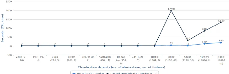
Xj | C) before it determines additional dependencies. Computing I(Xi ; C) takes linear time Θ(N)
proportional to the number of features. The class conditional mutual information is required to be calculated for each pair of features (total (N*N-1)/2 pairs) and runs in Θ(N2) time. Together they take Θ(N) + Θ(N2) time. Hence, the running time complexity for constructing the Model increases as the number of features increases. The situation gets worse when the given system has not many useful dependencies among features which at the end gives the classification accuracy similar to that of the Naïve Bayes Classifier.
39
In the next chapter, we study the implementation details for the Naïve Bayes Classifier and the Limited Dependence Classifier.
40
CHAPTER 6
Implementation
The Naïve Bayes Classifier as well as the Limited Dependence Classifier are written in Java. The following functionalities are provided by the implementation.
6.1 Functionalities
1. Reading data from source file (requires them to be in ARFF format) 2. Pre processing of data
3. K-fold cross validation and classification accuracy 4. Determining dependencies (Model construction) 5. Learning the Model
6. Model validation
These functionalities are written in separate java classes. Next, we cover the important implementation details of the above functionalities.
6.1.1 Reading Data from Source File
Input data is read from the given source file and is initially stored in a data structure of type Linked List of String Array. A collection of type Linked List provides the ability to access rows by their index. Later, (during pre-processing of source data) data is saved from two different perspectives: row oriented data and column oriented data. This setting provides easy access to entire row values
(observations) and to entire feature values (columns). 6.1.2 Pre Processing of Source Data
Pre processing of data includes reading input header, handling missing data, discretizing
41 6.1.2.1 Reading Header
Datasets used in the project are available in arff format. Arff file contains two sections: header part and data part. Header contains information such as name of the relation (type of dataset), list of features (called as attributes in arff file), their types (categorical or continuous) and range. Header of an example arff file for the Iris dataset is shown in Figure 5 [12].
Figure 5 Header part of an example arff file [12]
The input header routine reads the header and extracts all features (including class variable), their types (continuous or discrete) and range. If any feature has continuous range of type Integer and if the width of the range is ≤ 5, it is considered as discrete feature during further processing. This setting avoids unnecessary discretization of such features having integer values (which can be thought of as discrete values).
The data part of arff file contains set of pre-classified observations. Each observation has a value assigned (comma separated) to each feature including class variable, where the order of their
appearance follows the order with which they are defined in the header part. Figure 6 [12] shows the data part of the Iris dataset for the header shown in Figure 5. Here, each row corresponds to
observations while each column in each row corresponds to the features and the values they take. The class variable always appears as a last column.
42
Figure 6 Data part of an example arff file [12]
After extracting the header, data is saved in to a format suitable for various classification operations. These operations require data to be accessed from two different perspectives: access observations and access features. One data structure holds data row by row (observations) which makes it a convenient choice for operations such as handling missing data and testing the Model, while the other data structure holds data feature by feature (columns) which makes it a convenient choice for operations such as discretization, handling missing data and learning the Model.
6.1.2.2 Discretization of Features with Continuous Values
Classification datasets includes features with discrete and/or continuous values. Features with continuous values are discretized using the unsupervised equal-width binning approach [15]. A continuous range is divided into three equal sized bins (category). Bin size of 3 is applicable to all continuous features irrespective of their continuous range. Continuous features are scanned for column by column and each value is replaced by the bin (category) value they fall in. If any feature has missing values, they are omitted during discretization and are handled by ‘Handling missing data’ routine. The three new categories are designated by “_1”, “_2” and “_3” during further processing.
6.1.2.3 Handling Missing Data
Observations often have unobserved values for one or more features. Missing values are indicated by special characters (“?” and “<null>” in datasets from KEEL [10]). In order to replace missing
43
values, all observations are checked, one by one (rows). Any observation with missing values greater than or equal to 30% of the total value (total attributes in dataset) is removed from further
consideration. Next, every feature (including the class variable) is scanned for missing values (columns). Each feature takes values from their set of values (discrete range). Any feature with missing values greater than 30% of the total value (number of total observations) is removed entirely from further consideration; otherwise the missing values are replaced by the most frequently occurred value of that feature.
Scanning features for missing values does not allow us to correlate missing values with the other features’ missing values. Scanning observations for missing values first, followed by features allows us to look at missing values in any observation in an entire. This helps in ignoring observations which may reduce classification accuracy due to artificially substituted values in more number of features.
6.1.3 K- Fold Cross Validation and Classification Accuracy
Both Classifiers are validated using the 10-fold cross validation technique [11]. This technique repeatedly divides entire input data into two parts: training data and testing data. One such division gives us one fold. 10 folds (training and testing data) are formed from the input data, such that each observation becomes the part of test data exactly once in one of the fold. Observations from the input data are distributed randomly to the training and testing data of each fold (with no overlap across folds for the test data). During each fold, the training data is used to learn the Model while the testing data is used to validate the learnt Model.
During each fold, observations in test data are classified based on learnt Model and results (misclassified observations) are aggregated from previous fold. Classification accuracy is calculated using the following formula [9] and is reported (in percentage) at the end of the 10-fold cross validation.
44
Classification Accuracy = number of correctly classified instances total number of classifications
The standard deviation of misclassified observations from each fold is also reported at the end of 10-fold cross validation. This allows us to study the variation from the average of misclassified observations.
6.1.4 Determining Dependencies (Model Construction)
Naïve Bayes dependencies are quite straight forward and do not change from application to application. Each feature depends only on the class variable. On the other hand, dependencies for Limited Dependence Classifier are application specific and are determined using the algorithm
mentioned in Chapter 5. These dependencies are considered during learning and testing of constructed Model in each fold.
6.1.5 Learning the Model
Learning the Model requires information about feature dependencies as well as training data. We use the same Model during each fold. As each fold has different training data, the learnt Model in each fold differs. Both classifiers learn their Model using this functionality.
Learning the Model requires populating conditional probability tables for each feature.
Conditional probability tables have all possible combinations listed for values that features’ parents take and for each such combination a probability value is assigned to each value that the feature takes. These probability values are determined from the training data. We use Laplace correction [13] to avoid zero posterior probabilities.
45 6.1.6. Model Validation
Testing the Model requires information about feature dependencies as well as the testing data. For each observation in the test data, the posterior probability for each class category is determined. Here, we sum over the logarithm of the class variable’s marginal probability and each factor probability (P(Xi | Par(Xi)) instead of multiplication over these probabilities. This avoids integer underflow, as eq. 3.9
and eq. 5.4 multiplies these probabilities and gets smaller and smaller with each multiplication. The Model validation returns the number of incorrectly classified instances by comparing each classification result with the actual result from the test data.
Figure 7 presents a flow chart diagram for functionalities mentioned in section 6.1. The flow of Figure 7 is applicable to both Classifier algorithms.
46
47
Next, in chapter 7 we look at the classification results for several datasets and compare and contrast the Naïve Bayes and the Limited Dependence Classifier.
48
CHAPTER 7
Datasets and Results
The datasets used in this project are taken from KEEL data repository [10] which contains many types of classification datasets. I have taken “standard classification datasets” in which datasets have one or more features and only one class variable. In the next section, I describe each dataset.
7.1 Datasets 1) Titanicdataset
Type Titanic dataset
Description Contains observations about Titanic accident. Each observation outputs if a passenger survived or not
Features 3 discrete features
Class variable Class (has 2 categories) Total observations 2201
Training data size 1980
Test data size 221
Missing values No
2) Iris dataset
Type Iris dataset
Description Contains observations for Iris plant which are categorized into 3 types of Iris plant
Features 4 continuous features
Class variable Class (has 3 categories) Total observations 150
Training data size 135
Test data size 15
49 3) Car dataset
Type Car dataset
Description Contains observations which evaluates car model to one of the class category
Features 6 discrete features
Class variable Acceptability (has 4 categories) Total observations 1728
Training data size 1555
Test data size 173
Missing values No
4) Led7 dataset
Type Led7 dataset
Description Contains observations for 7-segment LED display which outputs digit (displayed on LED) as class category
Features 7 discrete features
Class variable Class (has 10 categories for 10 digits) Total observations 500
Training data size 450
Test data size 50
Missing values No
5) Nursery dataset
Type Nursery dataset
Description Contains observations which ranks nursery schools to one of the five class categories
Features 8 discrete features
Class variable Class (has 5 categories) Total observations 12690
Training data size 11421
Test data size 1269
50 6) Breast dataset
Type Breast dataset
Description Contains observations for breast cancer, which categorizes observations into two class categories
Features 9 discrete features
Class variable Class (has 2 categories) Total observations 286
Training data size 257
Test data size 29
Missing values No
7) Glass dataset
Type Glass dataset
Description Contains observations to categorize types of glass to one of the 7 categories based on their oxide content
Features 9 continuous features
Class variable Class (has 7 categories) Total observations 214
Training data size 192
Test data size 22
Missing values No
8) Tic-Tac-Toe dataset
Type Tic-Tac-Toe dataset
Description Contains observations which outputs win or lose for tic-tac-toe game. Observations include set of possible board configuration at the end of tic-tac-toe game. (‘X’ player always plays first)
Features 9 discrete features
Class variable Class (has 2 categories) Total observations 958
Training data size 862
Test data size 96
51 9) Magic dataset
Type Magic dataset
Description Contains observations which discriminate images generated by gamma from the images generated by Hadron initiated in the upper atmosphere.
Features 10 continuous features
Class variable Class (has 2 categories) Total observations 19020
Training data size 17118
Test data size 1902
Missing values No
10) Australian dataset
Type Australian dataset
Description Contains observations for Credit card applications which were either approved or denied
Features 6 discrete and 8 continuous features
Class variable Class (has 2 categories) Total observations 690
Training data size 621
Test data size 69
Missing values No
11) Zoo dataset
Type Zoo dataset
Description Contains observations which classifies given animal to one of the 7 class of animal
Features 16 discrete features
Class variable Class (has 7 categories) Total observations 101
Training data size 90
Test data size 11
![Figure 2 Probabilistic Graphical Model for extended-student-example [1]](https://thumb-us.123doks.com/thumbv2/123dok_us/8995816.2797412/19.918.291.652.450.605/figure-probabilistic-graphical-model-extended-student-example.webp)
![Figure 3 Probabilistic Graphical Model for Naïve Bayes Classifier [1]](https://thumb-us.123doks.com/thumbv2/123dok_us/8995816.2797412/26.918.176.735.112.308/figure-probabilistic-graphical-model-naïve-bayes-classifier.webp)
![Figure 6 Data part of an example arff file [12]](https://thumb-us.123doks.com/thumbv2/123dok_us/8995816.2797412/43.918.242.676.118.286/figure-data-example-arff-file.webp)