General-to-Specific Model Selection Procedures for Structural Vector Autoregressions

for Structural Vector Autoregressions

Department of Economics and Nuffield College, Oxford University.

[email protected] First version: December 2001

This version: March 2003

Abstract

Structural vector autoregressive (SVAR) models have emerged as a dominant research strategy in empirical macroeconomics, but suffer from the large number of parameters employed and the res-ulting estimation uncertainty associated with their impulse responses. In this paper we propose general-to-specific model selection procedures to overcome these limitations. After showing that single-equation procedures are efficient for the reduction of the SVAR, but generally not for the re-duction of its reduced form, the proposed rere-duction procedure is computer-automated using PcGets and its small-sample properties are evaluated in a realistic Monte Carlo experiment. The model se-lection procedure is shown to recover the DGP specification from a large unrestricted SVAR model with controlled size and power. The impulse responses generated by the selected SVAR are com-pared to those of the unrestricted and reduced VAR and found to be more precise and accurate. The proposed reduction strategy is then applied to the US monetary system considered by Christiano, Eichenbaum and Evans (1996). Although the selection process is hampered by the misspecification of the unrestricted VAR, the results are consistent with the Monte Carlo and question the validity of the impulses responses generated by the full system.

JEL Classification: C51, C32, E52.

Keywords: Model selection; Impulse responses; Vector autoregression; Structural VAR; Causal

or-der; Data mining.

1 Introduction

Over the last two decades, vector autoregressive (VAR) models have emerged as an important research tool for the empirical analysis of macroeconomic time series, partly because of the critique in Sims (1980) of traditional macro-econometric modelling. VARs have been widely exploited for the descrip-tion of numerous macroeconomic data sets, offering fruitful insight on the interreladescrip-tions between eco-nomic variables. The popularity of VARs is due to various advantages of the approach: First, the flexibility of the VAR framework in producing econometric models with useful descriptive characterist-ics, within which statistical tests of economically meaningful hypothesis can be executed. Secondly, the ease of the approach, as econometric models can be formulated and data characterized without having to invoke economic theory to restrict the dynamic relations between variables. Thirdly, the character-ization of macroeconomic models, as many completely specified economic models give rise to VAR representations as the reduced form of the variables of the system. Fourthly, the compatibility with quite a wide variety of hypotheses regarding the formation of expectations. Despite these advantages,

∗_{I am grateful to David Hendry for valuable comments and suggestions on previous versions of this paper.}

it is widely acknowledged in the literature that, in general, the innovations of VARs are not identified with the underlying structural errors due to the correlation of residuals across equations as in the case of instantaneous causality,. Therefore, the impulse responses generated by such a VAR do not possess a structural interpretation. While there is no unique best way to deal with this problem, a popular way of overcoming the problem, since Sims (1980), is the transformation of the residuals to orthogonal form by triangulating the system, which involves a causal ordering of the variables. The transformed VAR allows the interpretation of the evolution of the system as a function of the orthogonalized innovations in the variables of the system. A related approach to respond to the problem of interpreting VARs has been the development of structural vector autoregressions (SVARs), which introduce ‘theoretical’ restrictions to identify the underlying shocks. The SVAR approach tends to impose just enough restrictions to permit a coherent interpretation of the shocks to the system. In this paper we focus on SVARs made recurs-ive in contemporaneous variables. In contrast to SVARs in the spirit of Blanchard and Quah, 1989, identification is achieved by short-run restrictions specifying the causal ordering of the variables in the system.

SVAR models suffer from the fact that they rarely impose any restrictions upon the dynamics in their implied structural equations. For example, the relatively small structural VAR models of Bernanke and Blinder (1992) and Sims (1992) for the US economy have the distinctive feature that each struc-tural equation is saturated with lagged variables i.e. the dynamics are essentially unrestricted. In such a just-identified SVAR, the number of parameters grows with the square of the number of variables and quickly exhausts the degree of freedom (“curse of dimensionality”). Due to the large number of model parameters, the structural equations of the SVAR are not only estimated imprecisely, but also hard to interpret. These considerations point to the need for reductions of the systems which involve the utiliz-ation of exclusion restrictions upon the dynamics contained in each structural equutiliz-ation, so as to allow for easier interpretation of the system. It seems sensible to employ model reduction procedures, which so far have been mainly used in the single-equation framework. For the construction of a recursive SVAR of the Australian economy, Dungey and Pagan (2000) employ a modelling approach combining simplifications based on statistical tests and economic considerations. In this paper, we present a reduc-tion process proceeding by imposing zero restricreduc-tions according to the outcome of statistical tests and abstract from the use of economic theory for the derivation of overidentifying restrictions

The existing literature on VAR model selection has mainly focused on the selection of lag order,

p, of an otherwise unrestricted reduced-form VAR. In these selection procedures, a model is usually selected by an information criterion which penalizes the likelihood function for the number of paramet-ers. L ¨utkepohl (1991) discusses various strategies for selecting subset VAR models (i.e., VARs with zero constraints on the coefficients), which are based on the optimization of a specified model selec-tion criterion for a given maximal order of the VAR including full search, search over complete VAR matrices, top-down and bottom-up specification of the distributed lag lengths etc. Br¨uggemann and L ¨utkepohl (2000) consider step-wise-regression-type single-equation reduction paths where the critical value is chosen such that an acceptance of the null hypothesis guarantees a marginal increase in a given information criterion.

In this paper, we propose ‘General-to-specific’ (Gets) model selection procedures for SVAR models designed to overcome the limitations of just-identified SVAR models by reducing the number of required parameters. We will argue that the reduction and identification of SVAR models is a natural area for the application of Gets reduction procedures. The proposed reduction process is designed to ensure that the reduced SVAR model will convey all the information embodied in the unrestricted SVAR. This is achieved by a joint selection and diagnostic testing process: starting from the unrestricted, congruent general model, standard testing procedures are used to eliminate statistically-insignificant variables, with

diagnostic tests checking the validity of reductions, ensuring a congruent final selection. By reducing the complexity of the just-identified SVAR and simultaneously ensuring that the reduced SVAR will convey all the information embodied in the unrestricted VAR, the selected simpler, more compact model provides an improved statistical description of the economic world (see Hendry, 2000, for an overview of the so-called ‘LSE’ methodology). A further merit of this modelling approach is that it systematically checks for the presence of statistical misspecifications. In a substantial number of papers, the restrictions used to identify the VAR are imposed without establishing the congruence with the data (e.g. absence of regime changes and the constancy of the estimated coefficients: see, inter alia, Hendry and Mizon, 2000). For the economic interpretation of the SVAR and the generality of the derived impulse responses, it is therefore essential to ensure the congruence of the assumptions made.

The recent developments in automatic model selection initiated by Hoover and Perez (1999) sug-gests that the operational characteristics of some computer-automated model selection algorithms are excellent across a wide range of states of nature. For the computer implementation of the proposed model selection procedure for SVAR, we naturally focus on PcGets developed by Hendry and Krolzig (2001). PcGets automates general-to-specific (Gets) modelling for linear, dynamic, single-equation models based on the outlined theory of reduction. For a more detailed description of the algorithm see Hendry and Krolzig (2003). In Krolzig (2001) and Br¨uggemann, Krolzig and L ¨utkepohl (2002), computer-automated model selection algorithms such as PcGets were examined for the reduction of reduced-form VAR models and found to deliver reasonable results. It will be shown that single-equation procedures such as PcGets are efficient for the reduction of reduced-form VAR models under the con-dition of concon-ditional independence, and for recursive structural VAR models in general.

The structure of the paper is as follows: The following section (§2) defines the reduced-form and structural VAR model studied in this paper. §3 discusses the theoretical properties of Gets reduction procedures for the reduction of VAR processes. The small sample characteristics, foremost its selec-tion properties and the precision and accuracy of the generated impulse-responses, of the proposed Gets model-selection procedure as implemented by PcGets are then investigated by simulation. In the real-istic Monte Carlo experiment of§4, the data generating process is an over-identified trivariate SVAR(1) and the general unrestricted model is an SVAR(5) or VAR(5). An empirical illustration with a US mon-etary system based on Christiano et al. (1996) evaluating the usefulness of the proposed approach for the analysis of large macroeconomic data sets, follows in §5. In§6 we outline generalizations of the proposed modelling approach (i) for the selection of the causal order of the variables of the system, (ii) for the reduction of cointegrated time series models and (iii) for the search of simplifications as well as omitted variables in identified simultaneous equation models. Finally§7 concludes.

2 The vector autoregressive model

2.1 The reduced-form VAR

The basic model considered in the following is a vector autoregression possibly including deterministic terms and with independent Gaussian errors: then-dimensional time series vectory_tis generated by a stationary vector autoregressive process of orderp, denoted VAR(p) model,

yt=ν+ p X

i=1

Aiyt−i+εt, (1) wheret= 1, . . . , T, theAiandνare coefficient matrices and the initial values ofY₀= (y₀, . . . ,y_1−p)

unobservable Gaussian zero-mean vector white noise process with a time-invariant positive-definite variance-covariance matrixE[ε_tε0_t] =Σis given by:

εt∼NID(0,Σ). (2)

The infinite-order vector moving-average representation of the VAR in (1) is yt=µ+ ∞ X j=0 Ψjεt−j, (3) whereµ= (Pp_i=1A_i)−1ν andΨ(L) = I−Pp_j=iAiLi ₋₁

, such that for VAR(1) processes,Ψ_j =

Aj_{. The(k, l)-th elementψkl,j of the MA matrixΨj can be interpreted as the reaction of variablekin} response to a unit shock in variablel,jperiods ago.

The assumption that the shocks occur only in one of the variables, as implicitly made in this type of impulse response analysis, is fully justified under conditional independence, but problematic if the residuals are correlated. In the later case, the VAR can be readily transformed to interpret the evolution of the system as a function of orthogonalized innovations in any of the variables. Defineη∗_t =P−1ε_t

by decomposingΣasΣ=P P0, wherePis a lower triangular matrix, such thatη∗_t ∼NID(0,IK). The orthogonalized vector moving average representation is given by:

yt=µ+ ∞ X j=0 ΨjPP−1εt−j =µ+ ∞ X j=0 Φ∗_jη∗_t−j, (4) whereΦ∗₀ =Pand Φ∗_j =ΨjP. It is a well-known fact that orthogonalized impulse-responses, which are based on a Choleski decomposition of the variance-covariance matrix of the reduced-form VAR, are not invariant against changes in the (causal) ordering of the variables.

2.2 The structural VAR

The type of structural vector autoregressive (SVAR) processes considered in this paper is: Byt=δ+

p X

i=1

Γiyt−i+η_t, (5) where B, Γ_i and δ are coefficient matrices and the innovation process η_t is an unobservable Gaus-sian zero-mean vector white noise process with a time-invariant diagonal variance-covariance matrix E[η_tη0_t] =Ω:

η_t∼NID(0,Ω). (6)

The SVAR in equation 5 can be considered a particular simultaneous equation model in the spirit of the

Cowles approach. Particularly, it is a recursive system of the sort proposed by Wold (1949) and Strotz

and Wold (1960) and closely related to the concept of causal ordering introduced by Simon (1953). To recover the structural parameters it is useful to consider the structural VAR in equation (5) in its reduced-form. The relation to the VAR in (1) is given by:

Σ = B−1ΩB−10,

Ai = B−1Γ_i fori= 1, . . . , p, (7)

The uniqueness of the model for the given structure, which guarantees the estimableness of the structural parameters, is ensured by the following set just-identifying restrictions:

ωij = 0 fori6=j,

βii = 1 fori= 1, . . . , n, (8)

βij = 0 fori < j.

The infinite-order structural vector moving-average representation results from (3) by ε_t−j =

B−1_η t−j as: yt=µ+ ∞ X j=0 ΨjB−1ηt−j =µ+ ∞ X j=0 Φ_jη_t−j, (9) whereΦ(L) = B−Pp_i=1ΓiLi−1 withΦ0 =B−1. For a given causal ordering of the variables in the SVAR, the representation (9) differs from (4) only by the missing adjustment for the standard errors of theη_kt. In other words, the relation to (4) is given byη∗_t =Ω−12η_t.

3 General-to-specific reductions procedures for VAR models

VAR modelling is a natural area for the application of Gets: The unrestricted VAR(p) model constitutes the general unrestricted model (GUM) defining the model space to be searched for the unknown data generating process (DGP), which as we presuppose is a subset of the unrestricted VAR. Such systems can be analyzed one equation at a time, since every equation has the same set of regressors, but each variable is the regressand in turn.

The considered model selection procedure is of the form

ξ:χ→Ξ:Y→˜ξ=ξ(Y), (10)

whereχis the observation space,Ξis the model space, which collects all subsets models of unrestricted VAR, and Y is the observed sample. The selection problem consists of inclusion versus exclusion decisions for each coefficient of the full VAR and results in the binary selection vectorξ˜∈Ξ={1,0}n

with ones signaling inclusion and zeros elimination of the coefficient, nis the number of coefficients in the model. For a reduced-form VAR without deterministic terms we have thatn =K2p. Thus the dimension of model space, dim(Ξ) is 2K2p. We assume that the unrestricted VAR is congruent: the model space is consistent and includes the true selection vectorξDGP∈Ξ.

The Gets reduction process relies on a classical, sequential-testing approach (see, inter alia, Hendry, 1995 and 2000) . Different critical values are set for multiple and single selection tests, and for dia-gnostic tests. Denote byη the vector of significance levels for the misspecification tests (diagnostics) and byαthe vector of significance level for the various selection tests. During the specification search, the current specification is simplified only if no diagnostic test rejects its null. This corresponds to a likelihood-based model evaluation, where the likelihood function accepts the probability density func-tion of modelξ, only if the sample information coheres with the underlying assumptions of the model itself, i.e.min

˜

η(Y;˜θ_ξ)−η

<0, where the vector of diagnostic test statisticsp-values,˜η(Y;˜θ_ξ),is evaluated at the maximum likelihood estimateeθ_ξunder modelξ, and mapped into its marginal rejection probabilities.

Since jointly selecting and diagnostic testing eludes theoretical analysis, we approximate the Gets reduction process by:

˜ ξ = arg max ξ∈Ξc max θ 1 T 2L_T(θ_ξ)−c_T(α_T)n(θ_ξ) , (11)

where L_T(θ_ξ) is the log-likelihood resulting for the selected modelξ at the parameter vector θ_ξ for a sample Y_T of size T and n(θ_ξ) is the number of free parameters in the vector θ associated with selectionξ. The structure is similar to information criteria considered in the literature such as AIC with

cT = 2(see Akaike, 1985), BIC withc_T = logT (see Schwarz, 1978), and HQ withc_T = 2 log(logT)

(see Hannan and Quinn, 1979). But in contrast to those, the Gets selection process also ensures the congruence of a selected model, thus˜ξ ∈ Ξc whereΞc is the subset ofΞconsisting of all congruent models.

The statistical properties of the proposed model selection procedure will me measured as the de-viation of the selected model from the true model, ξ˜−ξDGP, usually expressed in terms of size, power and the probability finding the truth. For the framework considered here, the implications of the selection in terms of the accuracy and precision of impulse responses and predictions is at least as important. But before we analyze the properties of the procedure proposed here within a realistic Monte Carlo example in§4, we investigate the critical issue of complexity.

System procedures have the disadvantage that the number of subset models of a K-dimensional VAR(p) with an unrestricted variance-covariance matrix is given by2K2p(without deterministic terms). Even for model selection procedures based on a single criterion such as the usual information criteria, a full search over all possible candidates is computationally unfeasible: in a K-dimensional VAR(p) without deterministic terms there areK2pcoefficients, any full search requires the estimation of a total of2K2p subset models. Already for a four-dimensional VAR(p), the computational costs are immense: a full search procedure has to check 65,536 subset models of order one, 4,294,967,296 for p = 2,

2.8×1014 for p = 3, 1.8×1019 forp = 4 and so on. The challenge for sequential simplification and testing procedure for the system, comparable to PcGets in single equations, is even greater. Such is the chance to miss the DGP in such a high-dimensional model universe even with the most advanced multi-path encompassing search algorithm. It is therefore imperative to the restrict the dimensionality of the model universe by decomposing the selection problem into manageable sub-tasks. Single equation procedure do so by partitioning the model space intoKsubspaces,Ξ=Ξ₁×· · ·×Ξ_K, with dim(Ξ_k)= 2Kp. The critical question is whether there a loss in efficiency by analyzing the equations of a VAR once at a time using single-equation model selection algorithms rather than analyzing the VAR with a system procedure.

3.1 Gets reductions of reduced-form VAR models

We start by investigating Gets reductions of the reduced-form VAR(p) model defined in equation (1) in the case of a diagonal variance-covariance matrix, such that the equations of the system are unrelated to each other:

Proposition 1 (Reduction under conditional independence). Suppose that in the reduced-form VAR

defined in equation (1), the variance-covariance matrixΣis diagonal, i.e. allσ_ij = 0fori6=j. Then, all possible reductions of the system can be efficiently estimated by OLS, and model-selection procedures can operate equation-by-equation without a loss in efficiency.

Proof. Conditional independence of y_tconditional on its past Y_t−1 allows the factorization of the

probability density function ofy_tin terms of its marginals:

fy(yt|Yt−1) = n Y k=1

This implies that the log-likelihood functionL_T(θ)can be separated with regard to the parameters of interest,θ_k, of each equationk= 1, . . . , K of the system which can be varied freely:

LT(θ) = K X k=1 ( _T X t=1 lnf_yk(y_kt|Y_t−1;θ_k) ) = K X k=1 LkT(θk).

Consequently, all possible reductions of the system can be (asymptotically) efficiently estimated by single equation methods (OLS under normality), and reduction procedures can be applied equation-by-equation without a loss of (asymptotic) efficiency.

Proposition 1 states that the efficiency of single-equation model selection algorithms depends on the absence of instantaneous causality. In other words, if the variance-covariance matrix of the system is diagonal, i.e., allσ_ij = 0fori6=j,the system can be analyzed as collection of single-equation models. Hence, single-equation reduction procedures can be applied under optimality conditions. In VAR mod-els with instantaneous causality between the variables, the separability property of the log-likelihood function is lost: due to the contemporaneous correlation of variables in the system, the equations of the VAR are only seemingly unrelated to each other. Since eliminating a variable in one equation af-fects the others, single-equation model selection procedures are inefficient. This is directly related to the properties of the OLS estimation method, which is inefficient for subset VARs with non-diagonal variance-covariance matrices whereas full information maximum likelihood (FIML) and estimated gen-eralized least squares (EGLS) are (asymptotically) efficient. For the efficient reduction of interdependent reduced-form VAR models, Gets algorithms have to be implemented as system procedures.

3.2 Efficiency of Gets single-equation reduction procedures for SVAR models

In the following proposition, we argue that the recursive structure of SVAR models as defined in (5) re-establishes conditions for the efficiency of single-equation Gets reduction procedures. The crucial point is that the researcher does not aim to reduce the reduced-form VAR, but the recursive SVAR:

Proposition 2 (Reduction under causal ordering). Suppose that the GUM is a just-identified SVAR

of the form defined by (5). Then, all possible reductions of the SVAR can be efficiently estimated by OLS, and model-selection procedures can operate equation-by-equation without a loss in efficiency.

Proof. Causal ordering ofy_tallows the factorization of the probability density function ofy_tin terms

of marginals and conditionals:

fy(yt|Yt₋₁) =f_y1(y_1t|Yt₋₁)·f_y2|y1(y_2t|y_1t,Yt₋₁)·. . .·f_{yK|y1,...,yK−1}(y_Kt|y_1t, . . . , y_K−1t,Yt₋₁).

This implies that the log-likelihood functionL_T(λ) can be separated with regard to the parameters of interest,λ_k, of each equationk= 1, . . . , K of the system:

LT(λ) = T X t=1 lnf_y1(y_1t|Y_t−1,λ₁) + K X k=2 ( _T X t=1 lnf_{yk|y1,...,yk−1}(y_kt|y_1t, . . . , y_k−1t,Y_t−1,λ_k) ) = K X k=1 LkT(λk).

In other words, y₁, . . . , y_k−1 are weakly exogenous for the parameter vector λ_k = (β_k1, . . . , β_kk−1, γ_k1.1, . . . , γ_kk.p, ω2_k)0 of thek-th equation of the SVAR, which can be varied freely. Thus, reductions procedures for the SVAR can be implemented as single-equation techniques.

The great advantage of separability of the log-likelihood function for the recursive SVAR is that the model space generated by the just-identified SVAR which is of dimension2K(Kp+(K−1)/2), can be

searched inKsubspaces of dimensions2Kpto2Kp+(K−1). In§4 this case is studied in a Monte Carlo experiment, where we use PcGets as the computer-automated single-equation Gets reduction procedure.

4 Monte Carlo results

Although the sequential nature of the proposed model-selection process and its combination of variable-selection and diagnostic testing has eluded most attempts at theoretical analysis, an evaluation of the properties of the model-selection process can be achieved by simulation. In the Monte Carlo (MC) experiment considered here, the properties of the Gets reduction of SVAR models are studied under the conditions of proposition 2, which allows the optimal use of single-equation reduction procedures. For the computer implementation of the proposed model selection procedure we use PcGets.

4.1 Design of the MC

The DGP is a three-dimensional Gaussian SVAR(1) model with the causal orderingy_1t→y_2t→y_3t:    1 0 0 β21 1 0 β31 β32 1       y1t y2t y3t    =    γ11 0 γ13 0 γ₂₂ γ₂₃ 0 0 γ₃₃       y1t−1 y2t−1 y3t−1   +    η1t η2t η3t    (12) whereη_t∼NID       0 0 0   ,    ω2 1 0 0 0 ω2₂ 0 0 0 ω2₃      .

Its reduced-form is given by the VAR(1) model:    y1t y2t y3t    =    γ11 0 γ13 −β21γ11 γ22 γ23−β21γ13 −β21γ11 −β32γ22 γ33−β31γ13−β32γ23       y1t−1 y2t−1 y3t−1   +    ε1t ε2t ε3t    (13) whereε_t ∼ NID       0 0 0   ,    ω2 1 −β21ω12 −β31ω12 −β21ω12 ω22+β212 ω12 −β32ω22+β31β21ω21 −β31ω12 −β32ω22+β31β21ω21 ω23+β312 ω12+β322 ω22      .

We can think of the following ‘deep’ structure associated with recursive structure of the SVAR:

∆y_1t = −α(y_1t−1−y_3t−1) +η₁, ∆y_2t = −β(y_2t−1−y_3t−1−y_1t) +η₂, ∆y_3t = γ(y_2t−y_1t)−ρy_3t−1+η₃,

which forα = 0.4,β = 0.4, ρ = 0.4, andγ = 0.5, results in the following parameterization of the SVAR in (12):    1 0 0 0.4 1 0 0.5 −0.5 1       y1t y2t y3t    =    0.6 0 0.4 0 0.6 0.4 0 0 0.6       y1t−1 y2t−1 y3t−1   +    η1t η2t η3t    (14) η_t∼NID       0 0 0   ,    1 0 0 0 1 0 0 0 1      .

Thus the reduced form of the SVAR in (14) is given by the VAR(1) model:    y1t y2t y3t    =    0.60 0 0.40 −0.24 0.60 0.24 −0.42 0.30 0.52       y1t−1 y2t−1 y3t−1   +    ε1t ε2t ε3t    (15) εt∼NID       0 0 0   ,    1.00 −0.40 −0.50 −0.40 1.16 0.78 −0.50 0.78 1.74      .

With the eigenvalues ofA₁being0.672±0.351and0.376, the DGP is stationary with a zero mean. The sample sizeT is100and the number of replicationsMis1000.

In the Monte Carlo experiment we intend to evaluate the properties of the proposed Gets selection procedure. For the computer-automation of the reduction process, we use the conservative strategy of Hendry and Krolzig (2001). In addition to the selection properties discussed in the next section, the analysis of the simulation experiment will focus on the accuracy and precision of the resulting impulse-responses.

4.2 Selection properties

Search commences from a identified SVAR(5) or unrestricted VAR(5) model. Although the just-identified structural VAR and the unrestricted reduced-form VAR are identical models, they generate different model spaces. Therefore a Gets reduction process commencing from one of these will al-most surely select a different reduced model than when starting with the other. An important difference between the selected VAR and SVAR arises from the fact that in subset VAR models the variance-covariance matrix remains unrestricted during the search, while in subset SVAR models the free ele-ments of the matrix B will be subject to significance tests like any other coefficient of the system, resulting in a restricted variance-covariance matrix of its reduced form.

The selection properties of Gets reduction process proposed in this paper are reported in table 1 in terms of the ability of finding the DGP, the dominance of the selected model by the unknown DGP, as well as its size and power.

Given the characteristics of the DGP, the probability to find the DGP by PcGets is in between78.8%

and 86%for the SVAR, and22.2%to86%for the VAR. While naturally dependent on the design of DGP, these figures indicate that it is possible to retrieve the structure hidden in the data with a high probability. For the VAR, the success probabilities appear to be small, but they have to be compared to the probability of finding the DGP when starting the search from it, which is in between33.3%and

100%. As the overall probability to find or miss the DGP is not very informative, we check by an encompassing test whether the deviation of the selected model from the DGP results in a sound model that, based on statistically criteria, could not have been improved by knowing the truth. As long as

PcGets is able to find a model that is not dominated by the DGP itself, the reduction process has been

a success. If the specific model is dominated by the DGP, the search algorithm has failed. Our results indicate that the risk of finding a model which is dominated by the DGP is relatively small (2.6%to

4.2%) when compared to the probability that the selected model dominates the truth, which is 3 to 15 times higher. Note that, by construction, the outcome of the PcGets search algorithm will always beat the unrestricted VAR(5) model.

Next we analyze the ‘size’ and ‘power’ of the proposed model-selection process, namely the prob-ability of including variables that do not (do) enter the DGP in the selected model. The ‘size’ of PcGets (the average probability of selecting a nuisance regressor) is with1.57%to3.76%slightly higher than

Table 1 Selection properties.

Model SVAR VAR

Equation y_1,t y_2,t y_3,t y_1,t y_2,t y_3,t

DGP found when commencing from it 1.000 0.982 0.999 1.000 0.333 0.386

DGP found by PcGets 0.860 0.788 0.843 0.860 0.222 0.282 Non-deletion probability 0.140 0.189 0.155 0.140 0.325 0.264 Non-selection probability 0.020 0.056 0.021 0.020 0.738 0.675 DGP dominated by PcGets 0.099 0.153 0.113 0.099 0.554 0.550 PcGets dominated by DGP 0.026 0.042 0.031 0.026 0.033 0.038 Size 0.0157 0.0232 0.0169 0.0157 0.0376 0.0305

Size (reliability based) 0.0116 0.0165 0.0129 0.0116 0.0315 0.0263

Power 0.9880 0.9770 0.9920 0.9880 0.7227 0.7420

Power (reliability based) 0.9874 0.9727 0.9912 0.9874 0.7062 0.7250

the nominal size of a t-test which is1%. The size can be further improved by basing the selection decision on the reliability of the variables, which depends on the significance of the variables in two overlapping subsamples. In this case, the ‘size’ shrinks to1.16%–3.15%. The ‘power’ of PcGets (the average probability of selecting a DGP variable) is in between 99.2% and 72.27%. Overall, PcGets works more than satisfactorily despite the presence of collinearity among the regressors.

Having clarified the ‘success’ and ‘failure’ of PcGets in selecting a parsimonious representation of the structure found in the data, be proceed by checking how the selection properties of the proposed reduction strategy are translated into accuracy and precision of the impulse responses implied by the empirical model.

4.3 Impulse-response analysis

We now evaluate the properties the impulse-responses implied by the following models: (i) the true SVAR(1) defined in (14);

(ii) the pseudo-true VAR(1) defined in (15);

(iii) a just-identified SVAR(5) with intercept, which nests (14) and is identical to an unres-tricted VAR(5) with intercept nesting (15);

(iv) a Gets reduction of the just-identified SVAR(5) in (iii); (v) a Gets reduction of the VAR(5) in (v).

We are interested in the responses to structural and non-structural shock as laid out by the vector moving-average representations (3) and (9). The responses to the (normalized) structural shocksη∗_t =

Ω−1

2ηare given by:

∂yt+h

∂η∗

t0 =Φh =A

h_{P= (B}−1_Γ)h_B−1_Ω1

2. ₍₁₆₎

The responses to the non-structural shocksε_tresult as:

∂yt+h

∂ε0

t =Ψh =A

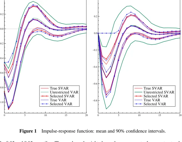
h _{= (B}−1_Γ)h_{. (17)} The impulse-responses functions implied by the models (i) to (v) are illustrated in figure 1, without loosing generality, for the response of the third variable y_3t+h to shocks in the first variabley_1tof the system. The graph on the left displays the responses ofy_3t+h to the structural shockη_1t. Plotted are their mean response (over theM = 1000replications) and their 90%confidence intervals as implied

0 5 10 15 20 −1.0 −0.8 −0.6 −0.4 −0.2 0.0 0.2

Reponse of y_3,t+h to a structural shock η_1,t in y₁

True SVAR Unrestricted VAR Selected SVAR True VAR Selected VAR 0 5 10 15 20 −0.8 −0.6 −0.4 −0.2 0.0 0.2

Reponse of y_3,t+h to a non−structural shock ε_1,t in y₁

True SVAR Unrestricted SVAR Selected SVAR True VAR Selected VAR

Figure 1 Impulse-response function: mean and 90% confidence intervals.

by the 0.05 and 0.95 quantiles. The graph on the right shows the responses to the non-structural shock ε1t. Note that the 90%confidence intervals for impulse-responses of the true and unrestricted SVAR as well as reduced-form VAR only reflect estimation uncertainty, while the confidence intervals for impulse-responses of the models selected by PcGets also account for the specification uncertainty.

Except for the subset VAR models, the mean impulse responses plotted in figure 1 are all close to each other, indicating that consistent estimates of the impulse responses can not only be obtained from unrestricted VAR models, but also from the selected SVAR model. Although the selected SVAR will always differ from the DGP with a positive probability, the squared biases (and confidence intervals) of its impulse responses are not much greater than for the true SVAR, when its structure but not its parameters are known and necessitates estimation. The bias problem caused by single-equation based reductions of the reduced-form VAR is nicely illustrated in figure 1: Some of the dynamic multipliers are falsely shrunk to zero as statistically insignificant autoregressive parameters are eliminated from the model

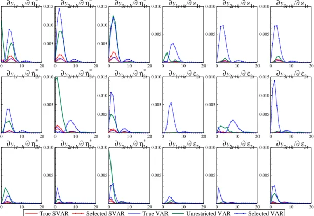
Figure 2 exhibits the squared bias of all structural and non-structural impulse responses. The bias can be defined as:

Bias[φ_ij,h] = ¯φ_ij,h−φ_ij,h (18) whereφ_ij,hdenotes the theoretical impulse response as implied by the model in equation (14) andφ¯_ij,h is the mean impulse response of one of the empirical models (i) to (v):

¯ φij,h= _M1 M X m=1 ˜ φ(_ij,hm). (19)

In a completely analogous fashion, the squared bias of the non-structural impulse-responses can be calculated. While for the true SVAR, the pseudo-true reduced-form VAR and the selected SVAR, the

0 10 20 0.005

0.010 ∂y1t+h/∂η * 1t

True SVAR Selected SVAR True VAR Unrestricted VAR Selected VAR

0 10 20 0.005 0.010 0.015 ∂y2t+h/∂η * 1t 0 10 20 0.005 0.010 0.015 ∂y3t+h/∂η * 1t 0 10 20 0.005 0.010 ∂y1t+h/∂ε1t 0 10 20 0.005 0.010 ∂y2t+h/∂ε1t 0 10 20 0.005 0.010 ∂y3t+h/∂ε1t 0 10 20 0.005 0.010 ∂y1t+h/∂η * 2t 0 10 20 0.005 0.010 ∂y2t+h/∂η * 2t 0 10 20 0.005 0.010 0.015 ∂y3t+h/∂η * 2t 0 10 20 0.005 0.010 ∂y1t+h/∂ε2t 0 10 20 0.005 0.010 ∂y2t+h/∂ε2t 0 10 20 0.005 0.010 0.015 ∂y3t+h/∂ε2t 0 10 20 0.005 0.010 ∂y1t+h/∂η * 3t 0 10 20 0.005 0.010 ∂y2t+h/∂η * 3t 0 10 20 0.005 0.010 ∂y3t+h/∂η * 3t 0 10 20 0.005 0.010 ∂y1t+h/∂ε3t 0 10 20 0.005 0.010 ∂y2t+h/∂ε3t 0 10 20 0.005 0.010 ∂y3t+h/∂ε3t

Figure 2 Squared bias of structural and non-structural impulse-responses.

accuracy of the non-structural impulse-responses is as good as that of the structural impulse responses, the unrestricted VAR looses accuracy when structural impulse responses are considered. This is because the Choleski decomposition fails to detect the structure in the variance-covariance matrix resulting from the zero parameters in theBmatrix.

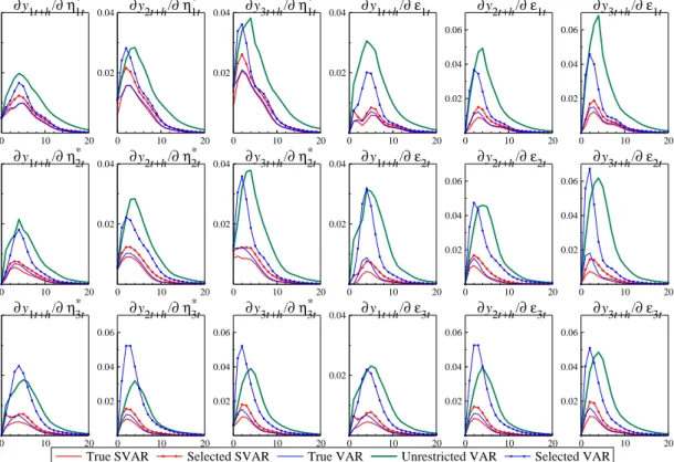
The uncertainty associated with the estimated impulse-responses can be measured by their variance: Var[φ_ij,h] = 1 M M X m=1 ˜ φ(_ij,hm)−_φ¯ ij,h ₂ , (20)

which for the Gaussian framework analyzed here, allows the construction of confidence bands in the usual way. For the non-structural impulse-responses, we analyze the elements ofΨ_h instead of Φ_h. Figure 3 plots the variances of estimated structural and non-structural impulse-responses for the model-ling strategies (i) to (v). Limiting the number of parameters by model reduction clearly helps to reduce estimation uncertainty. Consequently, the selected models produce more precisely estimated impulse responses than the full VAR. As seen in figure 1, the confidence bands for the impulse responses of the selected SVAR are much closer to those of the true SVAR than the ones of the just-identified SVAR. For this purpose, also single-equation based reductions of the reduced-form VAR are beneficial.

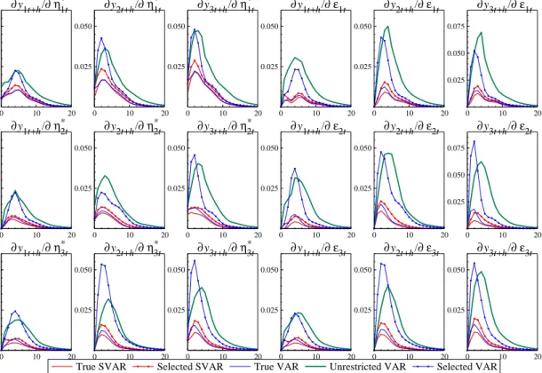
Finally, the overall error in estimating the impulse responses can be quantified by the mean square error: MSE[φ_ij,h] = 1 M M X m=1 ˜ φ(_ij,hm)−φij,h ₂

=Bias2[φ_ij,h] +Var[φ_ij,h] (21) for the response of y_i,t+h to a unit impulse to the structural shock term η_j,t and accordingly by MSE[ψ_ij,h] for the response to a non-structural shock in equation j, ε_j,t. The results are displayed

0 10 20 0.02

0.04 ∂y1t+h/∂η * 1t

True SVAR Selected SVAR True VAR Unrestricted VAR Selected VAR

0 10 20 0.02 0.04 ∂y2t+h/∂η * 1t 0 10 20 0.02 0.04 ∂y3t+h/∂η * 1t 0 10 20 0.02 0.04 ∂y1t+h/∂ε1t 0 10 20 0.02 0.04 0.06 ∂y_2t+h/∂ε_1t 0 10 20 0.02 0.04 0.06 ∂y_3t+h/∂ε_1t 0 10 20 0.02 0.04 ∂y1t+h/∂η * 2t 0 10 20 0.02 0.04 ∂y2t+h/∂η * 2t 0 10 20 0.02 0.04 ∂y3t+h/∂η * 2t 0 10 20 0.02 0.04 ∂y1t+h/∂ε2t 0 10 20 0.02 0.04 0.06 ∂y_2t+h/∂ε_2t 0 10 20 0.02 0.04 0.06 ∂y_3t+h/∂ε_2t 0 10 20 0.02 0.04 ∂y1t+h/∂η * 3t 0 10 20 0.02 0.04 0.06 ∂y_2t+h/∂η*_3t 0 10 20 0.02 0.04 0.06 ∂y_3t+h/∂η*_3t 0 10 20 0.02 0.04 ∂y1t+h/∂ε3t 0 10 20 0.02 0.04 0.06 ∂y_2t+h/∂ε_3t 0 10 20 0.02 0.04 0.06 ∂y_3t+h/∂ε_3t

Figure 3 Variance of structural and non-structural impulse-responses.

in figure 4 with the structural impulse responses on the left and non-structural impulse responses on the right.

As the MSE summarizes the effects of bias and variance, we get a clear picture of the relative precision and accuracy of the impulse response functions generated by modelling strategies (i) to (v). The true SVAR naturally delivers the best results throughout, followed by the pseudo-true VAR, and then the SVAR selected by PcGets. These three models consistently dominate the unrestricted VAR as well as the selected VAR. Forh <8, the unrestricted VAR and the equation-by-equation reduced VAR are close competitors, but for longer horizons, the MSEs of the subset VAR decline faster. Since the DGP and the estimated models are stable, the theoretical as well as the empirical impulse responses fade out with increasing distance between action and reaction. TheMSEs converge to zero with increasing

hproducing the hump shaped plots in figure 4.

The precision and accuracy of the model selection strategies are summarized in table 2 by calculating simple averages of the measures in (18) to (21) such as

MSE[φ] = 1 K2_H K X i=1 K X j=1 H X h=1 MSE[φ_ij,h], (22) for the non-structural impulse-responses and, analogously, MSE[ψ] for the non-structural impulse-responses. For the sake of convenience, the results have been normalized to one for the unrestricted VAR (just identified SVAR).

Table 2 provides a clear ranking of the modelling strategies: The true SVAR delivers the best results, followed by the pseudo-true VAR and the SVAR selected by proposed Gets model reduction procedure. The loss in accuracy due to ‘reconstruction’ of the unknown structure is very small when compared to the loss in accuracy when working with an unrestricted VAR (just-identified SVAR). Reducing the

reduced-0 10 20 0.025

0.050

∂y_1t+h/∂η*_1t

True SVAR Selected SVAR True VAR Unrestricted VAR Selected VAR

0 10 20 0.025 0.050 ∂y_2t+h/∂η*_1t 0 10 20 0.025 0.050 ∂y_3t+h/∂η*_1t 0 10 20 0.025 0.050 ∂y_1t+h/∂ε_1t 0 10 20 0.025 0.050 ∂y_2t+h/∂ε_1t 0 10 20 0.025 0.050 0.075 ∂y_3t+h/∂ε_1t 0 10 20 0.025 0.050 ∂y_1t+h/∂η*_2t 0 10 20 0.025 0.050 ∂y_2t+h/∂η*_2t 0 10 20 0.025 0.050 ∂y_3t+h/∂η*_2t 0 10 20 0.025 0.050 ∂y_1t+h/∂ε_2t 0 10 20 0.025 0.050 ∂y_2t+h/∂ε_2t 0 10 20 0.025 0.050 0.075 ∂y_3t+h/∂ε_2t 0 10 20 0.025 0.050 ∂y_1t+h/∂η*_3t 0 10 20 0.025 0.050 ∂y_2t+h/∂η*_3t 0 10 20 0.025 0.050 ∂y_3t+h/∂η*_3t 0 10 20 0.025 0.050 ∂y_1t+h/∂ε_3t 0 10 20 0.025 0.050 ∂y_2t+h/∂ε_3t 0 10 20 0.025 0.050 ∂y_3t+h/∂ε_3t

Figure 4 Mean square error of structural and non-structural impulse-responses.

Table 2 Precision and accuracy of impulse response functions.

structural impulse responses non-structural impulse responses Bias2 Variance MSE Bias2 Variance MSE

true SVAR (i) 0.1244 0.3106 0.2945 0.2353 0.1489 0.1498

pseudo-true VAR (ii) 0.1536 0.3559 0.3384 0.3204 0.2013 0.2025 selected SVAR (iv) 0.1992 0.4465 0.4252 0.3112 0.2604 0.2610 selected VAR (v) 0.9912 0.7916 0.8088 5.2855 0.6631 0.7105 unrestricted (S)VAR (iii) 1.0000 1.0000 1.0000 1.0000 1.0000 1.0000

form VAR with single-equation methods when the system is interdependent can cause a substantial bias; but it avoids the inflation in variance, which affects the full VAR so badly.

Altogether, our MC results highlight the dangers of (i) using impulse response analysis for unres-tricted, richly parameterized VAR models and (ii) employing single-equation reduction procedures for reduced-form VAR models when the conditions stated in proposition 1 are not met. While our Monte Carlo results suggest that the case for using Gets reductions of SVAR models for impulse-response ana-lysis is a strong one, it is still worth emphasizing two major limitations of the anaana-lysis presented here: First, a larger variety of DGPs has to be considered before we can conclude that the features found here are indeed systematic properties of proposed Gets procedure for the reduction of SVAR models. Secondly, it would be interesting to compare the Gets reduction procedure proposed in this paper with other model selection strategies discussed in the literature. For VAR models satisfying the conditional independence condition of proposition 1, Br¨uggemann et al. (2002) compared alternative computerized model-selection strategies and found a clear advantage of the PcGets algorithm in forecast comparis-ons. Similar competitions in the context of the SVAR modeling framework considered here are highly desirable.

5 Empirical illustration

To illustrate the proposed Gets procedures for SVARs, we will now use PcGets to analyze a small macro-econometric model for the US. The model is the monetary system introduced by Christiano et al. (1996) consisting of the log of real GDP,gdp, the log of the GDP deflator,p, the log of a commodity price index,pcom, the Fed funds rate,ff, the negative log of unborrowed reserves,nbrd, the log of total reserves,trand the log of M1,m1.

1960 1980 2000 8.0 8.5 9.0 gdp 1960 1980 2000 3.5 4.0 4.5 p 1960 1980 2000 3.5 4.0 4.5 pcom 1960 1980 2000 0.05 0.10 0.15 ff 1960 1980 2000 −4.0 −3.5 −3.0 −2.5 nbrd 1960 1980 2000 2.5 3.0 3.5 4.0 tr 1960 1980 2000 5.0 5.5 6.0 6.5 7.0 m1

Figure 5 The extended Christiano et al. (1996) data set.

The data are in levels and are plotted in Figure 5. The graphs show trending behavior in all variables. This could potentially cause a problem as, to date, PcGets conducts all inferences asI(0). The imple-mentation of cointegration tests and appropriate transformations would be useful (see the discussion in

§6). But most selection tests will in fact be valid even when the data areI(1), given the results in, inter

alia, Sims, Stock and Watson (1990). Only t- orF-tests for an effect that corresponds to a unit root

require non-standard critical values. Similarly, Wooldridge (1999) shows that diagnostic tests for the unrestricted model remain valid even for integrated time.

Christiano et al. (1996) considered an unrestricted reduced-form VAR(4) of the variables. Extending the data set to the period 1960 (i) to 1999 (iii), the VAR requires the estimation of 203 coefficients. Only few turn out to be significant at a5%significance level (see table 3), calling for reductions of the VAR. Using the liberal strategy of PcGets, the reduced-form VAR can be simplified to the subset VAR summarized in table 4. The results are in line with the earlier studies of Br¨uggemann and L ¨utkepohl (2000) and Krolzig (2001).

There are two major problems with this approach: First, the misspecification of all equations of the VAR except the price levelp(see table 5). There is a structural break in the middle of the sample period, which is presumably related to the Volcker deflation and affects the equations for commodity

Table 3 Unrestricted reduced-form VAR. variable ν gdp p pcom ff nbrd tr m1 lag 0 1 2 3 4 1 2 3 4 1 2 3 4 1 2 3 4 1 2 3 4 1 2 3 4 1 2 3 4 gdp . + . . . . . . . . . . . . − . . . . . . . . . . . + . . p − . . . . + − . − + . . . . − . . . + − . . . . + . . . . pcom . . . . . + − . . + . . − . . . . . . . . . . . . . . . . ff . + . . . . . − + + . . . + . + . . . . . . . . . . . + − nbrd . + . . − . . . . + . . . . . . . + − . . . − . . . . . . tr . − . . + . . . . . . . . . + . . . . . . + . . + + . . − m1 − − . . + . . . + − + − . − + − . . . . . + . . . + . . −

Legend: 0 Coefficient is set to zero. + Coefficient is positive and significant at the5%level.

. Coefficient is insignificant at the5%level. − Coefficient is negative and significant at the5%level.

Table 4 Subset reduced-form VAR.

variable ν gdp p pcom ff nbrd tr m1 lag 0 1 2 3 4 1 2 3 4 1 2 3 4 1 2 3 4 1 2 3 4 1 2 3 4 1 2 3 4 gdp 0 + 0 0 0 + 0 0 0 0 0 0 0 0 − 0 0 0 0 0 0 0 − 0 0 0 0 0 0 p − 0 0 + 0 + 0 0 − + 0 − 0 0 0 0 0 0 0 0 0 + 0 − + 0 0 0 − pcom 0 0 0 0 0 + − 0 0 + − 0 0 0 0 0 0 0 0 0 0 0 0 0 0 0 0 0 0 ff 0 + 0 − 0 0 0 − 0 + 0 0 − + 0 + 0 − 0 0 0 − 0 0 0 + 0 0 − nbrd 0 + 0 − 0 0 0 − 0 + 0 0 0 0 0 + 0 + − 0 0 − − 0 0 0 + 0 0 tr 0 − 0 0 + 0 0 0 + − 0 0 0 0 0 0 − 0 + 0 + + 0 0 + + − 0 − m1 − 0 0 0 + 0 0 0 + − 0 0 0 − + 0 0 0 0 0 0 + 0 0 0 + 0 0 −

Legend: 0 Coefficient is set to zero. + Coefficient is positive and significant at the5%level.

. Coefficient is insignificant at the5%level. − Coefficient is negative and significant at the5%level.

pricespcom, Fed funds rate,ff, unborrowed reserves, nbrd, total reserves,tr, and M1. The residuals ofgdp, pcom, ff and nbrd are non-Gaussian. There is some autocorrelation left in the case of M1, heteroscedasticity and ARCH effects can be found in thepcom and ff equations. Secondly, there is contemporaneous correlation among the residuals of the system. This violation of the condition for the efficiency of single-equation reduction procedures as stated in proposition 1 sheds some doubt on the properties of the reduction process, despite the fact that the over-identifying restrictions are not rejected by the LR test:χ2(143) = 150.44[0.3186].

Table 5 Misspecification tests: Unrestricted reduced-form VAR.

gdp p pcom ff nbrd tr m1 Chow(1979:4) 0.9264 0.5936 0.0076 0.0000 0.0000 0.0025 0.0074 Chow(1995:4) 0.5470 0.9800 0.8844 0.9833 0.9971 0.0479 0.4010 normality test 0.0078 0.2585 0.0000 0.0000 0.0000 0.8698 0.2836 AR 1-4 test 0.0492 0.0424 0.0414 0.1169 0.0107 0.5876 0.0006 ARCH 1-4 test 0.9620 0.5889 0.0001 0.0000 0.2996 0.5952 0.0656 hetero test 0.9710 0.6477 0.0414 0.0000 0.2898 0.3695 0.0763

Reported are the marginal rejection probabilities. Tests in bold are significant at1%.

Given the strong indication of instantaneous causality, it seems appropriate to adopt the causal or-dering imposed by Christiano et al. (1996),

gdp_t→p_t→pcom_t→ff_t→nbrd_t→tr_t→m1_t,

in their analysis of the effects of monetary policy shocks using orthogonalized impulse responses. The causal ordering is now used to set up the just-identified recursive SVAR. The involved sequential con-ditioning will admit the application of single-equation Gets reduction procedures.

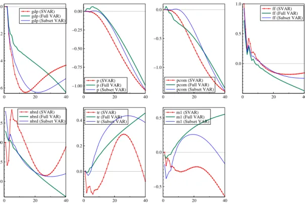
Table 6 Just-identified structural VAR.

variable ν gdp p pcom ff nbrd tr m1 gdp p pcom ff nbrd tr

lag 0 1 2 3 4 1 2 3 4 1 2 3 4 1 2 3 4 1 2 3 4 1 2 3 4 1 2 3 4 0 0 0 0 0 0 gdp . + . . . . − . . . . + . . p − . . . . + − . − + . . . . + − . . . − + . . . . . pcom . . . . + . . . . . + ff . . . . − + . . . . + . + . . . . + − + . + nbrd . . . . − . . . . − . . . + − . . . − . . . . . . + + tr . . . . − . − + . . + . . + + . . + + . . . . . . + − m1 − − + . . . . − + − . . . . + − . . . . . − . . . + . . . + + . − . +

Legend: 0 Coefficient is set to zero. + Coefficient is positive and significant at the5%level.

. Coefficient is insignificant at the5%level. − Coefficient is negative and significant at the5%level.

Table 7 Over-identified structural VAR.

variable ν gdp p pcom ff nbrd tr m1 gdp p pcom ff nbrd tr

lag 0 1 2 3 4 1 2 3 4 1 2 3 4 1 2 3 4 1 2 3 4 1 2 3 4 1 2 3 4 0 0 0 0 0 0 gdp 0 + 0 0 0 + 0 0 0 0 0 0 0 0 − 0 0 0 0 0 0 0 − 0 0 0 0 0 0 p − 0 0 + 0 + − + − + 0 − 0 0 0 0 0 0 0 0 0 + 0 − 0 0 0 0 0 0 pcom 0 0 0 0 0 − 0 0 0 + 0 0 0 0 0 0 0 0 0 0 0 0 0 0 0 0 0 0 0 0 + ff 0 0 0 − 0 0 0 − 0 0 − 0 0 + 0 + 0 0 0 0 0 − 0 0 0 + 0 0 0 + 0 + nbrd 0 0 0 0 0 0 0 0 0 0 0 0 0 − 0 0 0 + − 0 0 0 − 0 0 − + 0 0 0 0 0 + tr 0 0 0 0 0 − + 0 0 0 0 0 0 − + 0 0 + 0 0 0 + 0 0 0 + 0 − 0 0 0 0 + − m1 − 0 0 0 0 0 0 0 + 0 0 0 0 0 + 0 0 0 0 0 0 − 0 0 0 + 0 0 − + 0 0 − 0 +

Legend: 0 Coefficient is set to zero. + Coefficient is positive and significant at the5%level.

. Coefficient is insignificant at the5%level. − Coefficient is negative and significant at the5%level.

Table 6 reports the properties of the exactly identified SVAR which is observationally equivalent to the unrestricted VAR in table 3.1 Interestingly, conditioning removes the structural break in the commodity price,pcom_t, and the money demand equation,m1_tindicating the presence of cobreaking among the variables of the system. But, overall, table 8 shows that the (just identified) SVAR is also mis-specified stressing the necessity of continued research on the formulation of a congruent representation of the data.

Table 8 Misspecification tests: Just-identified structural VAR.

gdp p pcom ff nbrd tr m1 Chow(1979:4) 0.9264 0.5634 0.0450 0.0000 0.0000 0.0076 0.3329 Chow(1995:4) 0.5470 0.9730 0.6778 0.9797 0.9977 0.0698 0.6214 normality test 0.0078 0.2899 0.0001 0.0000 0.0000 0.1859 0.6647 AR 1-4 test 0.0492 0.0505 0.0644 0.0698 0.2272 0.0382 0.2558 ARCH 1-4 test 0.9620 0.6709 0.0001 0.0000 0.4869 0.4715 0.3567 hetero test 0.9710 0.7751 0.1622 0.0000 0.5533 0.0008 0.2833

Reported are the marginal rejection probabilities. Tests in bold are significant at1%.

The properties of the selected SVAR are summarized in table 7. The contemporaneous relationships are found to be:

pcom_t( p_t + ),ff_t( gdp_t + , pcom_t + ),nbrd_t( ff_t + ),tr_t( ff_t + , nbrd_t − ),m1_t( gdp_t + , ff_t − , tr_t + ).

The restrictions imposed by the reduction process can not be rejected by an LR test of the over-identifying restrictions: χ2(151) = 154.51 [0.4056].

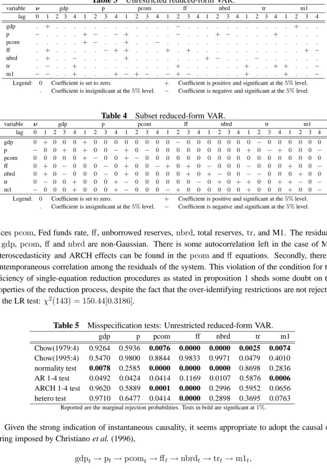
0 20 40 −0.6 −0.4 −0.2 0.0 gdp (SVAR) gdp (Full VAR) gdp (Subset VAR) 0 20 40 −1.00 −0.75 −0.50 −0.25 0.00 p (SVAR) p (Full VAR) p (Subset VAR) 0 20 40 −1.0 −0.5 0.0 pcom (SVAR) pcom (Full VAR) pcom (Subset VAR)

0 20 40 0.0 0.5 1.0 ff (SVAR) ff (Full VAR) ff (Subset VAR) 0 20 40 −0.50 −0.25 0.00 0.25 nbrd (SVAR) nbrd (Full VAR) nbrd (Subset VAR) 0 20 40 0.0 0.2 0.4 tr (SVAR) tr (Full VAR) tr (Subset VAR) 0 20 40 −0.5 0.0 0.5 m1 (SVAR) m1 (Full VAR) m1 (Subset VAR)

Figure 6 Response to a monetary policy shock.

Figure 6 shows the response of all system variables to a monetary policy shock, defined as a unit impulse in the Fed funds rate equation. Plotted are the responses derived from the (i) selected structural VAR, (ii) the selected reduced-form VAR and (iii) the full VAR as considered by Christiano et al. (1996). In case of a reduced-form VAR, the impulse-responses have been orthogonalized using the FIML (OLS) estimate of the variance-covariance matrix of the subset (full) VAR.

All three parametric models considered predict that an increase in the fed funds rate will cause a persistent drop in the level of GDP. However, while GDP is steadily falling in the unrestricted VAR model, the contraction in GDP bottoms out after 14 quarters in the over-identified SVAR and after 22 quarters in the subset VAR. The responses of the aggregate and commodity price indices show, after some delay, a smooth decline for the VAR and its reductions. The pattern of the own response of the fed funds rate over time is again very similar in the selected SVAR, the subset VAR and the full VAR. However, there are some striking differences in the impulse response functions of the selected models with regard to the monetary aggregates when compared to the impulse responses of the unrestricted system: While the full VAR predicts a secular decline or increase in the aggregates, the reaction of the negative log of unborrowed reserves and total reserves are mean-reverting in the structural VAR. Interestingly, the SVAR and the full VAR differ greatly regarding the responses in M1. Since we have shown earlier, that the reduced-form equation for M1 is misspecified (see table 5), whereas the structural equation for M1 was found to be congruent and stable over time (see table 8), we are inclined to put greater trust in the impulse response function derived from the selected SVAR. Finally, it is worth noting that since fewer parameters have to be estimated, the responses are estimated more precisely, making them a useful framework for tests for Granger causality etc.

6 Directions for further research

The Gets approach for the reduction of SVAR models presented in this paper has three important limit-ations: (i) the assumption that the causal ordering of the variable is known a priori, (ii) the stationarity of the data-generating process, and (iii) the recursive structure of simultaneous relations in the SVAR. In the following we briefly outline three directions for further research to overcome these limitations in a more general setting allowing for the applicability of the reduction procedure discussed here.

6.1 Selecting the causal order

The approach to the reduction of structural VARs proposed in this paper has been based on the as-sumption that the causal ordering of the variable is known a priori. In practice, the true causal order of the variables is usually unknown. While insight from the modeling context, particularly economic theory, can be extremely fruitful, there may be no unique ordering of the variables available. This raises the question whether sample evidence can be exploited for the selection of the causal order or, more precisely, the order of sequential conditioning.

While SVAR models which impose over-identifying restrictions can be tested, this is not the case for just-identifying restrictions. There is a rich literature on the determination of the design of the matrixBin (5) from the data by using the partial autocorrelations implied the estimated variance co-variance matrixΣ˜ of the reduced-form VAR (see, inter alia, Swanson and Granger, 1997, Reale and Tunnicliffe Wilson, 2002, and Selva and Hoover, 2002). These approaches have in common a two-stage approach: (i) the determination of the causal order based on the estimated covariance matrix of the unrestricted system, and then (ii) the reduction of the VAR dynamics conditional on (i).

In contrast, we suggest the reduction of the fully-identified SVAR for all possibleK!causal order-ings, and then the selection of the dominant model with the help of a consistent information criterion. If theK-dimensional vector of random variablesy_tis generated by a structural VAR in (1) overidentified by restrictions onΓ, then the reduced-form VAR and all other factorizations of the joint density should not be parsimoniously encompassing. A testing strategy would be preferable, but complications arise from the fact that even over-identified SVARs with different causal orders can have the same reduced form. Consider, for example, the following SVARs:

Byt = Γyt−1+ηt, E[ηtη0t] =Ω (23) B∗yt = Γ∗yt−1+η∗t, E[η∗tη∗t0] =Ω∗. (24) IfB−1Γ=B∗−1Γ∗ =AandB−1ΩB−10 =B∗−1Ω∗B∗−10 =Σ, then both models have the follow-ing reduced-form representation:

yt = Ayt−1+εt, withE[εtε0t] =Σ. (25) Hence, the SVARs (23) and (24) are observationally equivalent (see Hendry and Mizon, 2000, for more details).

6.2 Gets system reduction procedures for cointegrated VAR models

So far we assumed that the VAR is stable. Most economic data show stochastic trends, so that we should allow for integrated and possibly cointegrated processes. Since cointegration is a common feature of the variables in the system, and imposes nonlinear cross-equation restrictions on the parameters of the VAR, only system reduction procedures can be efficient. In the following, we outline a Gets system procedure for the reduction of cointegrated VAR models.