Exponential Smoothing Model Selection for Forecasting

Australia

Department of Econometrics

and Business Statistics

http://www.buseco.monash.edu.au/depts/ebs/pubs/wpapers/

Exponential Smoothing Model Selection for Forecasting

Baki Billah, Maxwell L King, Ralph D Snyder and Anne B Koehler

March 2005

Exponential Smoothing Model Selection for Forecasting

Baki Billah

Department of Epidemiology and Preventive Medicine Monash University, VIC 3800

Australia

Email: [email protected] Maxwell L. King

Department of Econometrics and Business Statistics Monash University, VIC 3800

Australia

Email: [email protected] Ralph D. Snyder

Department of Econometrics and Business Statistics Monash University, VIC 3800

Australia

Email: [email protected]

Fax: 613 9905 5474 Anne B. Koehler

Department of Decision Sciences and

Management Information Systems Miami Universiy

Oxford, OH 45056 U.S.A.

Email: [email protected]

Abstract:

Applications of exponential smoothing to forecast time series usually rely on three basic methods: simple exponential smoothing, trend corrected exponential smoothing and a seasonal variation thereof. A common approach to select the method appropriate to a particular time series is based on prediction validation on a withheld part of the sample using criteria such as the mean absolute percentage error. A second approach is to rely on the most appropriate general case of the three methods. For annual series this is trend corrected exponential smoothing: for sub-annual series it is the seasonal adaptation of trend corrected exponential smoothing. The rationale for this approach is that a general method automatically collapses to its nested counterparts when the pertinent conditions pertain in the data. A third approach may be based on an information criterion when maximum likelihood methods are used in conjunction with exponential smoothing to estimate the smoothing parameters. In this paper, such approaches for selecting the appropriate forecasting method are compared in a simulation study. They are also compared on real time series from the M3 forecasting competition. The results indicate that the information criterion approach appears to provide the best basis for an automated approach to method selection, provided that it is based on Akaike’s information criterion.

JEL CLASSIFICATION: C22

Keywords:

Model selection; exponential smoothing; information criteria; prediction; forecast validation

1. Introduction

The exponential smoothing methods are relatively simple but robust approaches to forecasting. They are widely used in business for forecasting demand for inventories (Gardner, 1985). They have also performed surprisingly well in forecasting competitions against more sophisticated approaches (Makridakis et al ,1982; Makridakis and Hibon, 2000).

Three basic variations of exponential smoothing are commonly used in practice: simple exponential smoothing (Brown, 1969); trend-corrected exponential smoothing (Holt, 1957); and Winters method (Winters, 1960). A distinctive feature of these approaches is that a) time series are assumed to be built from unobserved components such as the level, growth and seasonal effects; and b) these components need to be adapted over time when demand series display the effects of structural changes in product markets. As these components may be combined by addition or multiplication operators, 24 variations of the exponential smoothing methods may be identified (Hyndman, Koehler, Snyder and Grose, 2002). Given this proliferation of options, an automated approach to method selection becomes most desirable (Gardner, 1985; McKenzie, 1985).

Hyndman et al. (2002) provided a statistical framework for exponential smoothing based on the earlier work of Ord, Koehler and Snyder (1997). The framework incorporated stochastic models underlying the various forms of exponential smoothing and enabled the calculation of maximum likelihood estimates of smoothing parameters. It also enabled the use of Akaike’s information criterion (Akaike, 1973) for method selection. One issue not addressed was the preference for Akaike’s

information criterion over possible alternatives in Schwarz (1978), Hannan and Quinn (1979), Mallows (1964), Golub, Heath, and Wahba (1979), and Akaike (1970). An aim, therefore, is to determine whether Akaike’s information criterion (AIC) has a superior performance to its alternatives.

The exponential smoothing methods were traditionally implemented without reference to a statistical framework so that other approaches were devised to resolve the method selection problem. Prediction validation (Makridakis, Wheelwright and Hyndman, 1998) is one such approach. The sample is divided into two parts: the fitting sample and the validation sample. The fitting sample is used to find sensible values for the smoothing parameters, often with a sum of squared one-step ahead prediction error criterion. The validation sample is used to evaluate the forecasting capacity of a method with a criterion such as the mean absolute percentage error (MAPE). Another approach applies a general version of exponential smoothing on the assumption that it effectively reduces to an appropriate nested method when this is warranted by the data. Trend corrected exponential smoothing is applied to annual time series; Winter’s method is applied to sub-annual time series. A second aim is to gauge the effectiveness of these traditional approaches relative to the information criterion approach to method selection.

The plan of this paper is as follows. State space models for exponential smoothing and an approach to their estimation are introduced in Section 2. Criteria to be used in model selection and a measure for comparing resulting forecast errors are explained in Section 3. A simulation study is discussed in Section 4. An application of the model selection criteria to the M3 competition data (Makridakis and Hibon., 2000) is given

in Section 5. The paper ends with some concluding remarks in Section 6. 2. State space models

The state space framework in Snyder (1985), and its extension in Ord et al. (1997), provide the basis of an efficient method of likelihood evaluation, a sound mechanism for generating prediction distributions and the possibility of model selection with information criteria. Important special cases, known as structural models, that capture common features of time series such as trend and seasonal effects, provide the foundations for simple exponential smoothing, trend corrected exponential smoothing and Winters seasonal exponential smoothing. Of the 24 versions of exponential smoothing found in Hyndman et. al. (2002), the scope of this study is limited to three linear cases.

The focus is on a time series that is governed by the innovations model (Snyder, 1985): t t t y =h′x ₋₁+ε (2.1) α + = _t−1 t Fx x ε_t (2.2)

Equation (2.1), called the measurement equation, relates an observable time series value in typical period to a random -vector of unobservable components from the previous period. is a fixed -vector, while the

t

y t k x_t−1

h k ε_t, the so-called

innovations, are independent and normally distributed random variables with mean zero and a common variance _σ2_{. The intertemporal dependencies in the time series} are defined in terms of the unobservable components with the so-called transition equation (2.2). F is a fixed k×k ’transition’ matrix and α is a -vector of smoothing k

parameters.

The following special cases are termed structural models.

• Local Level Model (LLM) y_t =_lt−1 +ε_t

t t

where is a local level governed by the recurrence relationship

t l t αε + =_{l −1} l where 0≤α ≤1. It underpins the simple exponential smoothing method.

• Local Trend Model (LTM) y_t =_lt−1 +b_t−1+ε_t where is a local growth rate. The local level and local growth rates are governed by the equations t b t t t t =l −1 +b−1+ε

l and b_t =b_t−1 +βε_t where 0≤α ≤1 and α

β ≤ ≤

0 . Note that α′ =

[

]

• Additive Seasonal Model (ASM) y_t =_lt−1+b_t−1 +s_t−m+ε_t

t t

t b

, where is the local seasonal component. The local level, growth and seasonal components are governed by

t s t =l −1+ −1 +αε bt bt l , = ₋₁ +βε_t, t m t s t

s = ₋ +γε where m is the number of seasons in a year, 0≤α ≤1, β

α ≤ ≤

0 , and 0≤γ ≤1−α. In this case α′=

[

]

Traditionally, the smoothing parameters α β γ, , were set to fixed values determined subjectively by users on the basis of personal experience. The studies of Chatfield (1978) and Bartolomei and Sweet (1989) show that this can be problematic and that parameters are best estimated from data. Ord et al. (1997) recommend that estimates of the parameters be obtained by maximizing the conditional log-likelihood. For the class of linear state-space models (2.1) and (2.2) the conditional likelihood function

based on a sample of size n is given by

∑

where the errors are calculated recursively with a general linear form of exponential smoothing defined by the relationships ε_t = y_t −h′x_t−1 and x_t =Fx_t−1+α ε_t for

. 1 2

t= , , ,…n

This likelihood is not only a function of α but also of the unobserved random vector . The exact likelihood function is potentially obtained by integrating out of (2.3). An alternative strategy, however, is to treat as a fixed unknown quantity - hence the use of the term ‘conditional’. If the initial seed state vector is estimated first and entered into the conditional likelihood function, then the conditional likelihood is only maximized with respect to the parameter vector

0

x x₀

0 x

α . The conditional likelihood function was used for the studies in this paper for reasons that will be explained in the next section.

On obtaining the estimates xˆ₀ and αˆ

1

−

, the exponential smoothing algorithm may be used to obtain the corresponding estimate x of the state vector at the end of the sample. Point forecasts may be generated recursively with the equations

and for n ˆ j 1 ) ( ˆ_n j = ′ _n+j−

y hx xˆ_n+j =Fxˆ_n+j =1,2,_K,r where r is the prediction horizon.

3. Model selection approaches and a measure for comparing them

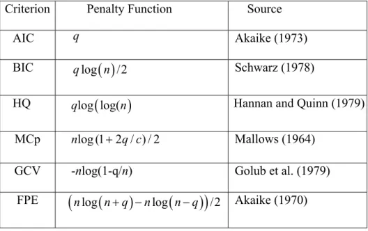
An information criterion has the general form logL(αˆ)− p(n,q) where p(n,q) is the so-called penalty function, being the number of free parameters. Various forms of q

the penalty have been suggested, as may be seen from Table 1. Note that is the number of free parameters in the smallest model that nests all models under consideration and . q∗ ∗ − =n q c

It is tempting to use the optimized value of the exact likelihood in the formulae for the various information criteria. However, the state variables in the models are generated by non-stationary processes so that the seed state vector has an improper unconditional distribution. One is confronted with a situation that is similar to Bartlett’s paradox (Bartlett (1957)) in Bayesian statistics. Exact likelihood values for models with different state dimensions are non-comparable and information criteria based on them will also be non-comparable. This is not an issue for the conditional likelihood because the use of improper unconditional distribution of the seed state vector is avoided. It is for this reason, that the conditional likelihood was used instead of the exact likelihood for estimating the parameter vector α . It is also for this reason, that the conditional likelihood was used with the information criteria.

No clear theory exists for deciding which of these information criteria is best suited for choosing the appropriate method of exponential smoothing. Thus, a simulation study was undertaken to compare them. The simulation also included a comparison with two other approaches for model selection. The prediction validation approach (Val) selects the model with the smallest MAPE for forecasting withheld data, and the encompassing model approach always selects LTM for annual data and ASM for quarterly and monthly data.

measure of forecasting effectiveness:

Median absolute prediction error as a percentage of the standard deviation of y_t

MdAPES =Median(APES)

      × = 100 deviaton Standard error Prediction t y Median =               × − − −

∑

This measure was chosen for several reasons. It had to be a unit free measure to permit comparisons between real time series measured in different units. It had to avoid the problems encountered with the MAPE (and its variations) for series values close to zero. Most importantly, it had to give a fair comparison on time series with different standard deviations. One would expect the forecast error to be larger when the standard deviation of a time series is large. The absolute prediction error as a percentage of the standard deviaton, APES, is a measure that will not produce larger values just because there is more variability in the time series. Thus, such time series will not necessarily cause an increase in the MdAPES just because of the larger variability. Inherently more variable time series can still have APES values near the median value and play a central in the evaluation process. In the comparisons, both simulated data and real data with different amounts of variability are included.

4. Simulation Study

The simulation study consisted of many experiments carried out under a wide variety of conditions. Depending on the type of data, the time series were generated by the three models: local level model (LLM), local trend model (LTM) and additive

seasonal model (ASM). Candidate values for the various factors in these models were: σ = 10, 20 (for all models)

n= 24, 40 (for LLM and LTM) n= 24, 60 (for quarterly/m=4 ASM) n= 48, 96 (for monthly/m=12 ASM) α = 0.1, 0.5, 0.9; _l0 =100 (for LLM) _, , ; _{ } (for LTM )      =       05 . 0 1 . 0 β α       1 . 0 4 . 0       1 . 0 7 . 0 , 1 100 0       =      o b l      5 100 , , ; _{ } ; 1 . 0 05 . 0 1 . 0           =           γ β α           2 . 0 1 . 0 4 . 0           3 . 0 1 . 0 7 . 0 , 1 100 0       =      o b l      5 100 = A 0, 25, 50 (for ASM)

The various combinations of these factors leads to 180 scenarios for the simulation study.

The 180 scenarios were repeated 10 times (i.e. 10 trials) so that the study consisted of 1800 simulation experiments. Each experiment consisted of the following four steps:

1. Generate a time series, from a specified model, consisting of a) a tuning sample of a specified size and b) an evaluation sample for r succeeding periods. For annual data

n

6

=

r , for quarterly data r =8, and for monthly data .

18

= r

2. Using the conditional likelihood function, fit a collection of models (the LLM and LTM for annual data; additionally the ASM model for quarterly and monthly data) to the tuning sample.

3. Select the best model by one of the model selection approaches

is best according to the specified information criterion. b. For the prediction validation approach (Val)

i. Withhold the last r years of the tuning sample and fit the local level model, local trend model, and additive seasonal model to the first n-r values by maximizing the conditional likelihood function.

ii. Choose the model with the smallest MAPE for the forecasts of the r periods of withheld data.

c. For the encompassing approach (Enc)

i. Choose the local trend model for annual data.

ii. Choose the additive seasonal model for quarterly and monthly data.

4. Using the estimates from Step 2 for the model chosen in Step 3

i. Generate predictions for each of the r periods in the evaluation sample.

ii. Calculate the absolute prediction error as a percentage of the standard deviation of the tuning sample (APES) for each of the time periods in the evaluation sample.

For Step 1 only, the seed seasonal components in the ASM were generated from the equation )s_j−m = Asin(2jπ/m , j=1,2,_K,m, where is the seasonal amplitude and

m is the number of seasons in a year.)

A

In Step 2 the estimates for the initial seed state vector x₀ were found by: Average of the first three values (for LLM)

Global trend for the first five observations (for LLT)

Global trend and seasonal dummies for the first two years of data (for ASM)

The results of the simulation are shown in Tables 2 through 4. Table 2 contains results that use all 180 scenarios in each of the 10 trials. For each of the eight model selection approaches, Table 2(a) displays the median absolute prediction error as a percentage of the standard deviation (MdAPES), and Table 2(b) contains the interquartile range (IQR) of APES, a unit free measure for the variability of the prediction errors. Parts (c) and (d) of Table 2 show the individual ranking of the eight model selection approaches on each trial and the mean ranking for all ten trials, where a rank of 1 is best. The AIC and FPE have the smallest mean ranking of 2.2 for the MdAPES, and the AIC has the least variability for the prediction errors as shown by smallest mean ranking of 3.0 for the IQR of the APES. However, the actual values of the MdAPES are very close for many of the criteria. Only the BIC and the Prediction Validation (Val) approaches are consistently worse than the other methods with respect to the median and the IQR. In particular, both these approaches are worse than the encompassing approach, which is to always choose the LTM for annual data and the ASM for quarterly and monthly data. This is a surprising result for BIC and Val and will be examined more closely by looking at the subcategories in Tables 3 and 4 and on real data.

Comparisons within subcategories that are formed by splitting the forecasts for all the simulated time series into forecasts over short and long horizons, forecasts from large and small tuning samples, and forecasts for annual, quarterly, and monthly data are presented in Tables 3 and 4. Table 3 shows the values of the MdAPES, and Table 4

shows the mean ranking of MdAPES. In Table 4, the mean ranking for the AIC is never worse than the other methods and is usually much better. The BIC and Val continue to be ranked very low and always much worse than the AIC. For seasonal data, both the BIC and Val are worse than the Enc, which always chooses the ASM. However, for annual data both are better than Enc. While the AIC has better rankings compared to other approaches, the actual percentages are frequently quite close except for BIC and Enc. FPE is almost identical to the AIC. This latter result is to be expected since they are the same asymptotically. It is interesting that the encompassing model does so well compared to the all other criteria in all subcategories other than annual data.

The use of simulated data does raise the criticism that in real life the true model is unknown. Furthermore, real series are not so well behaved as the simulated series. This happens even when random errors and outliers are included in the simulated series. In the next section, we investigate how forecasting performance is affected by the eight approaches to model selection on real data.

5. Application to the M3 Competition Data

In this section the eight model selection approaches are applied to the M3 competition data (Makridakis and Hibon, 2000) to see whether the results of simulated data carry through for real data. In order to apply all eight approaches to the same set of time series, it was necessary to remove time series that were too short. Each time series had a tuning sample of a specified size n and an additional evaluation sample of size r

where r =6 for annual data, r =8 for quarterly data, and r =18 for monthly data. For the prediction validation appraoch, it was necessary to fit models to n−r observations. Thus, since the fitting sample was reduced from n to n-r values and

observations were also needed to estimate the initial seed values for the unobservable components, it was decided to require for annual, for quarterly data, and for monthly data. These requirements left 1452 of the 2829 times series in the M3 data for use in the comparative study.

20 ≥ n n≥28 72 ≥ n

The procedures that were described in Steps 2 and 3 of Section 3 for the simulation study were applied to the 1452 time series from the M3 competition data. The results are shown in Tables 5 and 6. Table 5 displays the median absolute prediction error as a percentage of the standard deviation of the time series (MdAPES) and the interquartile range of the APES for all the time series, and Table 6 has the MdAPES for subcategories. Although not as strong, findings similar to those in the simulation study are seen in the comparison of applying the approaches to real data. The AIC continues to have the smallest MdAPES and smallest IQR for the APES. The BIC and Val remain the worst two criteria except in the case of model selection for annual data. Since real data in not well-behaved as simulated data, one would not expect the evidence to be as strong for the M3 data.

6. Conclusions

Simulated time series and real time series from the M3 competition provide very similar information when they are used to compare approaches for model selection. The AIC appears to be the best of the information criteria for selecting among the major exponential smoothing methods. Other studies for ARIMA models have not shown the AIC to be superior to the BIC (see for example Koehler and Murphree, 1985). However, these studies have been trying to distinguish the number of AR and MA terms rather than the amount of differencing. The ARIMA models that are equivalent to LLM, LTM, and ASM differ by the amount of differencing as well as

the number of parameters. Recall that in order to be able to compare the exponential smoothing models, the AIC and BIC are computed using the conditional likelihood function rather than the exact likelihood.

The comparisons on the simulated and real data both indicate that the prediction validation approach is a less desirable choice. The tables show that prediction validation is especially poor for small samples and monthly data. It makes sense that approaches that use all the data to fit the models in the selection process should be better than prediction validation, especially for short time series.

The encompassing approach frequently does well in the comparisons. However, it is not as good as the AIC. Since computers have such great capacity and speed now, it is not a burden to do the extra work that is required by the AIC over always using LLT for annual data and ASM for monthly data. Overall, the results support the use of the AIC to choose models for exponential smoothing.

7. References

Akaike, H. (1970). Statistical predictor identification, Annals of Institute of Statistical Mathematics, 22, 203-217.

Akaike, H. (1973). Information theory and an extension of the maximum likelihood principle. In: B. N. Petrov and F. Csaki (eds.), Second International Symposium on Information Theory(pp. 267-281). Budapest: Akademiai Kiado.

44, 533-534.

Bartolomei, S. M. & Sweet, A.L. (1989). A note on a comparison of exponential smoothing methods for forecasting seasonal series, International Journal of Forecasting, 5, 111-116.

Brown, R. G. (1959). Statistical Forecasting for Inventory Control. New York: McGraw Hill.

Chatfield, C. (1978). The Holt-Winters forecasting procedure, Applied Statistics, 27, 264-279.

Gardner, E. S. (1985). Exponential smoothing: the state of the art, Journal of Forecasting, 4, 1-28.

Golub, G. H., Heath, M. & Wahba, G. (1979). Generalized cross-validation as a method for choosing a good ridge parameter, Technometrics, 21, 215-223.

Hannan, E. J. & Quinn, B. G. (1979). The determination of the order of an autoregression, Journal of the Royal Statistical Society, Series B, 41, 190-195.

Holt, C. C. (1957). Forecasting Trends and Seasonal by Exponentially Weighted Averages, ONR Memorandum No. 52, Carnegie Institute of Technology, Pittsburgh, USA (published in International Journal of Forecasting 2004, 20, 5-13).

Hyndman, R. J., Koehler, A. B., Snyder, R. D. & Grose, S. (2002). A state space framework for automatic forecasting using exponential smoothing methods.

International Journal of Forecasting, 18, 439-454 .

Koehler, A.B. & Murhpree, E. S. (1988), A comparison of the Akaike and Schwarz Criteria for Selecting Model Order, Applied Statistics, 37, 187-195.

Makridakis, S., Andersen, A., Carbone, R., Fildes, R., Hibon, M., Lewandowski, R., Newton, J., Parzen, E., & Winkler, R. (1982). The accuracy of extrapolation (time series) methods: results of a forecasting competition, Journal of Forecasting, 1, 111-153.

Makridakis, S. & Hibon, M. (2000). The M3-Competition: results, conclusions and implications, International Journal of Forecasting, 16, 451-476.

Makridakis, S., Wheelwright, S. C., & Hyndman, R. J. (1998). Forecasting: methods and applications. New York: John Wiley & Sons.

Mallows, C. L. (1964). Choosing variables in a linear regression: a graphical aid, presented at the Central Regional Meeting of the Institute of Mathematical Statistics, Manhattan, Kansas.

McKenzie, E. (1985). Comments on ‘Exponential smoothing: the state of the art’ by E.S. Gardner, Journal of Forecasting, 4, 32-36.

Ord, J. K., Koehler, A. B. & Snyder, R. D. (1997). Estimation and prediction for a class of dynamic nonlinear statistical models, Journal of the American Statistical Association, 92, 1621-1629.

Schwarz, G. (1978). Estimating the dimension of a model, The Annals of Statistics, 6, 461-464.

Snyder, R. D. (1985). Recursive estimation of dynamic linear statistical models,

Journal of the Royal Statistical Society, Series B, 47, 272-276.

Winters, P. R. (1960). Forecasting sales by exponentially weighted moving averages,

Table 1. Alternative Penalty Functions

Criterion Penalty Function Source

AIC q Akaike (1973)

BIC _qlog

( )

HQ _qlog

(

)

GCV -nlog(1-q/n) Golub et al. (1979) FPE

(

(

)

(

)

)

Table 2

All time series in simulated data (10 trials of 180 scenarios)

(a) Median absolute prediction error as a percentage of the standard deviation (MdAPES) Selection Trial Approach 1 2 3 4 5 6 7 8 9 10 AIC 25.3 21.0 21.9 18.6 25.8 26.7 25.1 22.9 21.6 26.1 BIC 27.0 21.0 22.9 20.1 26.7 28.6 27.2 24.4 23.3 27.9 HQ 25.6 20.2 21.9 19.0 26.1 27.2 25.0 22.9 22.2 25.9 MCp 25.3 21.0 22.1 18.8 25.7 26.4 25.1 23.0 21.6 26.3 GCV 26.0 21.5 23.6 19.1 25.8 25.1 25.5 23.1 22.1 25.8 FPE 25.5 21.0 21.8 18.6 25.8 26.7 25.1 22.8 21.6 26.1 Enc 26.3 21.6 23.9 18.9 25.7 25.1 25.9 23.2 22.1 25.9 Val 27.3 23.2 25.9 20.4 26.9 27.5 28.1 24.4 25.2 27.4

(b) Interquartile range of the APES (IQR)

Selection Trial Approach 1 2 3 4 5 6 7 8 9 10 AIC 50.3 46.3 43.0 41.3 58.8 55.4 50.5 47.2 44.3 54.1 BIC 51.5 47.7 44.2 44.1 61.3 61.7 54.8 51.5 51.6 55.0 HQ 51.3 46.8 43.4 41.5 58.8 54.9 50.6 47.3 46.5 53.1 MCp 50.3 46.1 43.0 40.7 58.9 55.2 50.5 47.4 44.3 54.3 GCV 52.1 48.0 45.1 41.3 57.7 51.9 50.8 44.9 44.2 52.5 FPE 50.9 46.3 42.7 41.3 58.8 55.4 50.5 46.6 44.3 54.1 Enc 52.6 48.0 44.5 41.2 57.7 52.4 51.6 44.8 44.2 52.5 Val 56.8 57.6 48.8 45.1 62.4 61.1 58.5 48.9 52.9 57.1

( c) Ranking of the MdAPES

Selection Trial Approach 1 2 3 4 5 6 7 8 9 10 Mean AIC 1 2 2 1 3 4 2 2 1 4 2.2 BIC 7 5 5 7 7 8 7 7 7 8 6.8 HQ 4 1 2 5 6 6 1 3 6 2 3.6 MCp 1 4 4 3 1 3 2 4 1 6 2.9 GCV 5 6 6 6 3 1 5 5 4 1 4.2 FPE 3 2 1 1 3 4 2 1 1 4 2.2 Enc 6 7 7 4 1 1 6 6 4 3 4.5 Val 8 8 8 8 8 7 8 8 8 7 7.8

(d) Ranking of the IQR

Selection Trial Approach 1 2 3 4 5 6 7 8 9 10 Mean AIC 1 2 2 4 4 5 1 4 3 4 3.0 BIC 5 5 5 7 7 8 7 8 7 7 6.6 HQ 4 4 4 6 3 3 4 5 6 3 4.2 MCp 2 1 3 1 6 4 2 6 4 6 3.5 GCV 6 7 7 3 1 1 5 2 2 2 3.6 FPE 3 3 1 5 5 6 3 3 5 5 3.9 Enc 7 6 6 2 2 2 6 1 1 1 3.4 Val 8 8 8 8 8 7 8 7 8 8 7.8

Table 3

Median absolute prediction error as a percentage of the standard deviation (MdAPES) for subcategories of the simulated data

(a) Forecast horizon

Selection Trial Horizon Approach 1 2 3 4 5 6 7 8 9 10 short AIC 18.6 15.5 15.5 13.0 17.7 19.2 17.3 17.7 15.6 20.7 BIC 19.6 16.2 17.1 14.5 19.4 20.1 18.6 19.2 17.1 21.9 HQ 19.1 15.4 15.6 13.4 17.8 19.3 17.3 17.8 16.2 20.3 MCp 18.6 15.4 15.6 13.2 17.6 19.0 17.3 17.7 15.6 20.9 GCV 18.4 15.4 16.3 13.8 17.0 17.5 17.5 17.6 15.9 20.4 FPE 18.7 15.5 15.5 13.0 17.7 19.2 17.3 17.8 15.6 20.7 Enc 18.5 15.4 16.3 13.6 16.9 17.5 17.6 17.6 15.9 20.9 Val 20.1 18.4 19.3 15.0 19.1 19.3 19.0 19.2 19.0 20.6 long AIC 34.5 26.7 32.1 25.8 40.5 38.2 36.8 30.7 29.4 36.6 BIC 38.1 26.3 32.5 28.2 39.6 41.2 39.3 33.1 32.9 39.4 HQ 35.8 25.7 32.5 26.2 40.0 38.4 36.9 31.5 31.1 35.9 MCp 34.5 26.8 32.2 26.1 40.5 37.5 36.8 30.8 29.4 37.1 GCV 35.8 27.8 33.6 27.6 40.7 35.7 36.5 30.8 31.6 36.4 FPE 34.9 26.7 32.1 25.8 40.5 38.2 36.8 30.7 29.4 36.6 Enc 36.3 27.8 33.8 27.1 40.7 36.0 36.9 31.0 31.4 36.5 Val 38.8 28.5 33.7 28.6 39.2 36.9 41.8 31.3 31.5 38.9

Note: annual (short 1-3, long 4-6); quarterly (short 1-4, long 5-8); monthly (short 1-9, long 10-18)

(b) Sample size Selection Trial Sample Approach 1 2 3 4 5 6 7 8 9 10 small AIC 34.7 35.6 34.7 29.6 47.2 43.6 36.2 38.7 34.5 41.5 BIC 39.4 36.5 36.5 34.3 47.6 48.3 38.5 42.1 37.4 46.1 HQ 36.3 35.4 34.8 30.9 47.7 43.5 35.9 39.3 36.1 41.6 MCp 34.7 35.5 34.8 29.0 47.2 44.0 36.2 38.9 34.5 41.8 GCV 36.1 38.1 36.7 31.3 47.0 41.0 35.8 38.1 35.4 41.0 FPE 35.8 35.6 34.6 29.6 47.2 43.6 36.2 38.5 34.5 41.5 Enc 36.4 37.9 36.6 31.0 47.0 41.2 36.4 38.2 35.2 41.3 Val 42.7 39.2 38.6 31.5 43.4 43.8 40.0 38.9 37.9 44.9 large AIC 17.0 11.4 12.8 11.6 11.1 15.8 17.3 13.2 13.5 15.6 BIC 17.5 12.0 12.7 11.9 11.7 16.9 18.2 13.4 13.7 16.3 HQ 17.1 11.1 12.4 11.5 11.4 16.3 17.3 13.3 12.9 15.7 MCp 17.0 11.4 12.8 11.6 11.0 15.1 17.3 13.2 13.5 15.6 GCV 17.4 11.8 13.0 11.3 11.2 14.8 17.5 13.4 13.4 15.7 FPE 17.0 11.4 12.8 11.6 11.1 15.8 17.3 13.2 13.5 15.6 Enc 17.3 11.8 13.0 11.3 11.2 14.8 17.5 13.5 13.4 15.7 Val 17.2 13.2 14.4 13.0 14.0 16.7 19.0 14.5 15.0 15.6

Note: annual (small 24, large 40), quarterly (small 24, large 60); monthly (small 48, large 96)

Table 3 (continued) (c) Type of data Selection Trial Type Approach 1 2 3 4 5 6 7 8 9 10 annual AIC 48.4 32.6 42.5 45.3 46.9 43.2 44.6 48.5 36.5 31.4 BIC 49.7 32.1 43.2 46.0 46.9 42.3 45.2 49.3 37.4 39.0 HQ 48.4 32.8 43.7 45.3 46.9 42.3 45.7 48.5 36.5 31.4 MCp 48.4 32.6 42.5 45.3 46.9 43.2 44.6 48.5 36.5 31.4 GCV 48.4 35.3 44.6 41.1 50.0 46.1 43.6 40.2 38.9 32.3 FPE 48.4 32.6 42.5 45.3 46.9 43.2 44.6 48.5 36.5 31.4 Enc 50.7 34.7 43.5 38.6 50.0 45.9 50.1 41.1 37.3 35.7 Val 52.3 25.2 42.1 41.8 53.6 40.8 46.8 40.2 36.5 31.2 quarterly AIC 23.5 23.3 23.5 24.9 22.7 26.1 24.1 24.7 26.4 29.1 BIC 23.5 23.3 22.9 27.0 22.7 26.3 24.4 26.4 27.8 29.3 HQ 23.5 23.3 22.9 26.7 22.7 26.4 24.2 25.0 26.5 29.3 MCp 23.5 23.4 23.5 24.6 22.7 26.4 24.1 25.1 26.4 29.6 GCV 24.3 23.2 25.7 24.4 21.9 24.5 25.2 23.8 24.7 29.0 FPE 23.5 23.3 23.2 24.9 22.7 26.1 24.1 24.7 26.4 29.1 Enc 24.4 23.2 25.7 24.4 21.9 24.5 25.2 23.8 24.7 29.0 Val 24.5 24.7 25.6 27.1 23.6 27.5 25.5 26.8 28.1 29.7 monthly AIC 23.7 18.9 18.5 14.4 25.3 24.6 23.0 19.5 18.6 24.0 BIC 26.1 19.2 19.8 16.2 26.6 28.1 26.1 21.3 19.5 26.0 HQ 24.5 18.1 18.6 14.8 25.7 25.1 22.6 19.3 18.8 23.6 MCp 23.7 18.9 18.7 14.4 25.3 24.4 23.0 19.5 18.6 24.2 GCV 24.4 19.5 19.2 15.3 25.6 22.6 23.2 20.7 19.4 24.0 FPE 24.1 18.9 18.5 14.4 25.3 24.6 23.0 19.4 18.6 24.0 Enc 24.4 19.5 19.2 15.3 25.6 22.6 23.2 20.7 19.4 24.0 Val 26.3 21.6 23.1 16.3 26.8 25.1 27.0 21.1 22.2 25.4 Table 4

Mean ranking of the MdAPES for subcategories

Selection Forecast Horizon Sample Size Type of Data

Approach short long small large annual quarterly monthly

AIC 2.8 2.3 2.7 2.5 2.4 2.9 1.9 BIC 7.3 6.2 7.0 6.6 5.3 4.6 7.1 HQ 4.4 4.0 4.4 3.5 4.2 4.9 3.3 MCp 3.4 3.7 3.9 3.1 4.1 5.0 3.0 GCV 2.8 4.4 3.5 4.4 5.2 2.7 4.4 FPE 4.2 3.7 3.7 4.0 5.2 4.6 3.2 Enc 3.8 5.5 4.2 5.0 5.9 3.5 5.4 Val 7.3 6.2 6.6 6.9 3.7 7.8 7.7

Note: annual (short 1-3, long 4-6); (small 24, large 40) quarterly (short 1-4, long 4-8); (small 24, large 60) monthly (short 1-9, long (10-18); (small 48, large 96)

Table 5

All time series from the Makridakis M3 Competition

Selection Approach MdAPES IQR(APES) AIC 36.2 61.9 BIC 37.5 63.2 HQ 37.0 61.9 MCp 36.3 61.6 GCV 36.7 63.4 FPE 36.2 62.0 Enc 36.6 64.2 Val 37.6 64.1 Table 6

Subcategories of time series from the Makridakis M3 Competition

Selection Selection

Category Approach MdAPES Category Approach MdAPES

Forecast short AIC 27.7 Type of annual AIC 45.8

Horizon BIC 28.7 Data BIC 45.0

HQ 28.3 HQ 45.0 MCp 27.7 MCp 45.8 GCV 28.7 GCV 47.2 FPE 27.7 FPE 45.8 Enc 28.8 Enc 49.2 Val 28.9 Val 45.0

long AIC 47.0 quarterly AIC 35.2

BIC 48.1 BIC 35.8 HQ 47.6 HQ 35.3 MCp 47.2 MCp 35.2 GCV 47.5 GCV 35.6 FPE 47.0 FPE 35.2 Enc 47.2 Enc 35.6 Val 48.6 Val 33.9

Sample small AIC 47.6 monthly AIC 36.0

Size BIC 47.7 BIC 37.7

HQ 47.6 HQ 37.1 MCp 47.3 MCp 36.2 GCV 49.2 GCV 36.5 FPE 47.6 FPE 36.0 Enc 49.4 Enc 36.2 Val 50.2 Val 38.3

large AIC 35.2 Note:

BIC 36.8 Annual Quarterly Monthly

HQ 36.2 Forecast

MCp 35.4 Horizon

GCV 35.6 short 1-3 1-4 1-9

FPE 35.3 long 4-6 5-8 10-18

Enc 35.5 Sample Median (divides small vs large)