Paper Number: 01-1029 An ASAE Meeting Presentation
Precision Agriculture: A Break-Even Acreage Analysis
Jean-Marc GandonouAgricultural Economics 339 C.E. Barnhart Building
University of Kentucky Lexington, KY 40546-0276
Timothy S. Stombaugh, Ph.D. Biosystems and Agricultural Engineering
214 C.E. Barnhart Building University of Kentucky Lexington, KY 40546-0276 Carl R. Dillon, Ph.D.
Agricultural Economics 403 C.E. Barnhart Building
University of Kentucky Lexington, KY 40546-0276
Scott A. Shearer, Ph.D., P.E. Biosystems and Agricultural Engineering
218 C.E. Barnhart Building University of Kentucky Lexington, KY 40546-0276
Written for presentation at the 2001 ASAE Annual International Meeting
Sponsored by ASAE Sacramento Convention Center
Sacramento, California, USA July 30-August 1, 2001
Abstract. Before engaging in precision agriculture (PA) it is important to determine the least cost strategy of obtaining the technology. A key decision to make is whether to buy the requisite equipment or custom-hire the services. Using marginal analysis in a partial budgeting framework, the study determines the breakeven acreage necessary to economically justify the purchase of PA equipment versus custom hire. The results suggest that the break-even acreage between the decision to custom hire versus the purchase of the PA equipment is about 430 ha (1,060 ac) for field mapping, grid soil sampling and a single product (nutrient) variable rate application.
Keywords. Economic analysis, grid soil sampling, GPS, precision farming, variable-rate application.
The authors are solely responsible for the content of this technical presentation. The technical presentation does not necessarily reflect the official position of the American Society of Agricultural Engineers (ASAE), and its printing and distribution does not constitute an endorsement of views which may be expressed. Technical presentations are not subject to the formal peer review process by ASAE editorial committees; therefore, they are not to be presented as refereed publications. Citation of this work should state that it is from an ASAE meeting paper. EXAMPLE: Author's Last Name, Initials. 2001. Title of Presentation. ASAE Meeting
Precision Agriculture: A Break-Even Acreage Analysis
J. Gandonou, T.S. Stombaugh, C.R. Dillon, and S.A. Shearer
Introduction
Agriculture is increasingly becoming a computerized information-based industry. Perhaps the best example of the trend is the evolution of precision agriculture (PA). PA can be defined as a comprehensive system designed to optimize agricultural production by carefully tailoring soil and crop management to correspond to the unique condition found in each field while maintaining environmental quality (Blackmore et al., 1994). This technology is based upon the availability of geographically referenced data, and the use of this data in the decision-making process. Processing of this spatial data makes PA a powerful management and decision tool.
The production and economic data can be collected, sorted and analyzed to create information. The progressive accumulation of information used to manage and control the production process eventually results in knowledge. This knowledge creates a competitive advantage in the market place. Thus, PA has become both a management tool, as well as a means of increasing profitability for early adopters. Ultimately, producers who started collecting data early will mostly likely be the ones who will first be able to successfully use this technology as it matures, given the importance of historical data in the decision-making process. It is this lack of sufficient historical data to the early adopters of PA that has resulted in unexpected results. Many of the early adopters have made drastic and inappropriate changes in their management practices based on one year of spatial data (McGill). Those experiences have proven PA to be in a large measure about data management.
Instead of the increased profitability that would have been expected by early adopters of PA, a few economic studies have found PA to be unprofitable. Perhaps the first extensive review detailing the profitability of PA was published by Lowenberg-DeBoer and Swinton (1997). They reported that out of 17 studies, 30% found PA to be unprofitable and 35% had mixed results. However, a more recent review by Dayton and Lowenberg-DeBoer reported that only 12% of the 108 studies reviewed reported a negative net return and 29% a mixed result. These results suggest there was a higher success rate among the early adopters of PA. If so, that might help explain the initial modest adoption rate of PA technology in spite of the fascination that it has generated since its introduction. Bullock et al. linked the slow rate of adoption to low profit potential, which was attributed in part to the absence of PA historical data available to producers, and the high cost of the equipment. High equipment cost has resulted in the adoption of PA mainly on large farms (Popp and Griffin), in part due to the high fixed cost. Spreading this cost over a larger acreage improves profitability. Therefore, it is important to what size of farm is required to justify the investment in PA equipment versus the alternative of custom hiring.
The purpose of this study is to provide potential PA adopters with insights into the least cost alternative between PA equipment ownership versus custom hire to assist in their
decision-making process. Furthermore, the break-even acreage analysis developed in this study can be adapted to specific conditions of interest beyond the example presented. The outcome should enable farmers to develop a least-cost strategy in building site-specific management capacity and databases. For some farmers the least cost strategy will be to hire custom services to build databases and gain experience. For others with sufficient acreage, equipment ownership will be the most cost effective entry point in PA. However, the equipment ownership for those farmers may be limited to the equipment complement necessary to perform some, but not necessarily all, PA operations. In this study, a break-even acreage decision tool will be developed that will allow farmers to know when to purchase their own PA equipment and when to custom hire the service. While the focus here is an example of common grain producer, it can be easily adapted to different types of enterprises.
Background Information
The main advantage of PA is it allows farmers to spatially manage fields using a geographic information system (GIS). Use of GIS involves the analysis of multiple layers (or coverages) of data. There are variuos starting points for GIS data collection in PA. The availability of accounting data on the field-by-field basis is probably the first recommended layer of data useful before engaging in PA (Lowenberg-DeBoer, 1995; McGill, 1997). It allows the producer to evaluate the additional gain or loss resulting from the adoption of PA. Crop yield mapping and soil related characteristics are also very important data, and often constitute an entry level in PA for many farmers. Thus, spatial management is made possible through grid sampling and soil mapping techniques. By grid sampling and soil mapping, it becomes possible to establish a clear overview of the nutrient availability over the entire field. This spatially detailed soil fertility data enables the use of variable rate application (VRA). VRA enables nutrient application levels to be varied spatially within the field. Consequently, this technique enables the producer optimize fertilizer use for improved profitability. Ancillary to the profit motive is potential to improve environmental quality by eliminating the over-application of nutrients and chemicals. PA also enables the collection of detailed production response data for spatially accurate management decision making via yield monitoring and mapping. Thus, PA adoption enables managers to move from macro (field level average) to a micro (grid or management zone specific) management of production. Micro-management enables optimizing inputs to obtain the best possible return on the investments in machinery, seed, fertilizer and pesticides. The expected increase in profitability resulting from the adoption and use of PA is perhaps the primary focus of most PA economic investigations.
There are two common assumptions made in production economics. The first is that the primary goal is to maximize profit. The second assumption is that a risk-return tradeoff exists wherein a higher expected profit is often accompanied with greater risk. In their study on adoption, profitability and potential trends of PA in Arkansas, Popp and Griffin (2000) found that the expectation of an increase in net return was among the most important reasons that motivated early adopters of PA technology. However, according to their review of the literature on the profitability of PA, Lowenberg-DeBoer
and Swinton (1997) noted that for the six PA studies found to be profitable, undercounting costs was the primary reason for the positive results. In their own study (“Economics of Site-Specific Management in Agronomic Crops”), they found the adoption of PA to be unprofitable for the specific case they examined. Profitability must be determined on a farm-by-farm basis, suggesting that individualized analyses are required.
Producers need decision tools that are applicable across broad and varying conditions. Although the conditions surrounding the determination of the general profitability of PA are individualized and farm dependent, the costs of engaging in PA are less likely to differ from producer to producer. Furthermore, cost minimization is essential for profit maximization. Consequently, for producers who decide to engage in PA, it becomes necessary to investigate the least-cost strategy of adopting the technology. Reduction of production costs (Popp and Griffin, 2000) appears to be the leading reason for early adopters to engage in PA. The expectation in most cases is that adopting PA technology will lead to a reduction in the quantity of input used while increasing yield. However, while some inputs (e.g. fertilizer) may be reduced with PA, others (e.g. equipment use) can increase. Thus, the additional cost incurred from switching from traditional "field-level" to "precision agriculture" becomes critical because it balances against the reduction of other inputs and increased yield. While some may consider the expense of PA equipment ownership to be prohibitive to its adoption, they may fail to recognize that custom hiring may be a practical alternative. Thus, the additional cost of engaging in PA can either appear in the form of an investment in PA equipment, or as a custom-hire rate. To minimize the cost of switching from traditional farming to PA, the manager needs to know when to choose either of the options. Partial budgeting can serve as a means of economically comparing two alternative decisions. Break-even analysis can be coupled with the partial budgeting technique to develop a widely applicable decision tool.
Partial budgeting is the common economic tool used in the literature for assessment of the profitability of PA. It will be used within this manuscript as well. It enables the calculation of the expected profit from a proposed change in a farm’s operation. "It is capable of analyzing only two alternatives at a time; the current situation and a proposed alternative” (Kay and Edwards, 1999). In this manuscript the two alternatives to be analyzed are "custom hire" versus "purchase of PA equipment." From the partial budget set up a break-even relationship is established to obtain the break-even point, in this case acreage or land area. The break-even result enables the producer to know at what point it is no longer profitable to purchase the PA equipment. Partial budgeting and break-even analysis provide the basis for analysis.
Analysis Framework and Data Requirements
This study relies upon marginal economic analysis conducted through partial budgeting, which is in turn simplified into a break-even acreage determination. This analysis requires the collection of physical data constituting the necessary equipment compliment and economic data
including the resulting ownership and operating expenses, as well as custom hire rates. Data, both physical and economic, will be discussed following the model development.
Model Development
Partial budgeting is a method of estimating the costs and benefits that result from a proposed change in the operation of a farm business. The aim is to estimate the change that will occur in farm profit as a result of initiating a change in the farm plan and therefore organize a marginal economic analysis framework. The potential benefits or enhanced profitability associated with a change in the farm operation includes additional revenue and reduced costs. The potential costs or reduction in profitability associated with a change in the farm operation includes additional costs and/or reduced revenue. By focusing only on factors that change as a result of the alternative operation, a partial budget provides an estimate of the marginal effect on profit (benefits less costs). Insights to the estimated economic effects of a proposed change are thereby afforded by a partial budget.
While the partial budget method alone is sufficient to solve the problem for the case at hand, break-even analysis permits one to develop a general benchmark for a more robust, broadly applicable, tool. Specifically, a producer must possess sufficient acreage to reduce the average fixed cost of equipment ownership to justify its purchase. Custom hiring would be more cost effective for a farmer with a small farm size in terms of acreage. But, at some point, a farmer with enough land would be expected to benefit more by owning the equipment than through custom hire. Given the fact that this minimum cost decision is largely a function of farm size, solving for the break-even acreage point of indifference between the two alternatives provides a benchmark for farmers to use in making a least cost strategy decision. Farmers whose field size is close to the break-even acreage result would want to analyze their personal situation with more attention using the framework established herein. On the other end, a producer whose field size is considerably below (above) the break-even acreage result may be more comfortable with custom hiring (owning equipment) to engage in the chosen PA activity.
The partial budget is used to establish a breakeven relationship between the cost of purchase or custom hire of the PA equipment. The breakeven point is a function of farmed area (acreage) and has been discussed previously (e.g. Kay and Edward, 1999). The related equation is the point where ownership costs are equivalent to custom hiring costs and is expresses as follows:
where TFC is the total fixed cost of PA equipment ownership; TVC is the total variable costs associated with operating owned PA equipment; CH is the custom hired rate and A is total area of land where PA is to be practiced. Algebraically solving for A results in:
TFC/(CH-TVC) = A
The break-even acreage was calculated based on this formula. For farmers with fewer acres, custom hiring is more cost effective than with greater acreage levels associated with ownership being more economical. The break-even acreage is also a function of the PA operations to be performed, and therefore requires a description of the machinery complement, or physical data.
Physical Data
The physical data consists of the additional equipment set that a farmer will need to engage in PA practices. Choosing the appropriate equipment set to make this move often becomes a challenge given that the technology is still maturing. This often results in incompatibility problems for farmers. Expert opinions from engineers in the Department of Biosytems and Agricultural Engineering of the University of Kentucky were necessary to conduct the study. The equipment combination detailed next is among the most efficient and least expensive currently available. It is designed to accommodate grain production activity and includes field machinery, computer hardware and software. The equipment combination used in this study enables single-product (nutrient or lime) VRA.
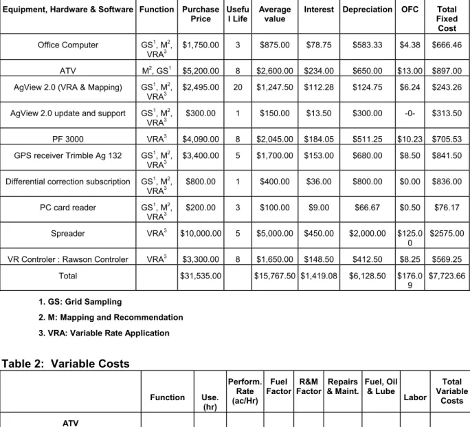
The requisite equipment for conducting the PA operations in this study includes an all terrain vehicle (ATV), box spinner spreader, rate controller, GPS receiver, PC card, task computer, office computer, and mapping and recommendation software. The applications of this equipment are presented in Table 1 and discussed next.
The ATV is used to collect soil samples in the field. The box spinner spreader applies the correct amount of fertilizer or lime according to the recommendation. For this application it is assumed that the box spreader is fitted to a used, dedicated truck chassis. The rate-controller is an essential component of the VRA equipment. The Ag. Leader Precision Farming (PF) 3000 will be used to accomplish the in-field control activities of the task computer. It is a general-purpose monitor/controller that can be moved from the combine to ATV. Finally, VRA is mechanically executed via a Rawson Controller. This controller consists of a hydraulic valve, motor and the associated electronic controls. Communication with the task computer is accomplished via a serial interface.
Other components of the PA equipment include the GPS receiver, the PC card and a task computer. The GPS receiver allows the farmer to instantaneously determine the position of the PA equipment as it operates in the field. This information is fed to the task computer for use in control of product application rates. However, a stand-alone GPS can have errors as high as 100-meters, which is unacceptable for PA field operations. To improve receiver accuracy farmers are often required to subscribe to a differential correction service. The differential correction data allows the GPS receiver to achieve accuracies in the sub-meters or the sub-meter range. The spatial data collected in the field with the GPS receiver and task computer are transferred to the office computer using a PC card. Processing of the data to generate maps and recommendation files requires that farmers invest in a new office computer. Early adopters have frequently realized that simply buying PA equipment and software was not enough. To store and analyze this data for map generation, farmers need a desktop or office computer with adequate memory, improved processing speed, a high-quality color monitor and color printer. The minimum requirement for the new computer include: a Pentium III processor, 128 Megabytes of RAM, 10 Gigabyte hard disk, enhanced video/display card, 19" monitor and a color printer. The PA software specified for collecting and processing data was AgView, Version 2.0. This software was used to collect field data, perform data analysis, and generate application recommendations. This software also facilitates communication with the VRA controller and GPS receiver for field-level control of application. This complement of equipment, computer hardware and software constitutes the minimum necessary to perform the selected PA operations.
Economic Data
Economic data were used to compute the ownership and operating costs associated with the PA equipment. The potential benefits and cost reductions made possible by PA are offset by additional costs to engage in the technology. Investments involve fixed (or ownership) and variable (or operating) costs. Because of farm size, not all farmers will be able to justify the fixed costs associated with PA investment as compared to the alternative of custom hiring PA operations.
Fixed (or ownership) costs associated with PA equipment include depreciation, interest, insurance and taxes. Depreciation expense is calculated based on the straight-line method and is a function of purchase price, salvage value and useful life. It is obtained by dividing the purchase price of the equipment by its useful life given that salvage value equals zero. Insurance and taxes represent 1.25% of purchase price for the spreader and 0.25% for all other equipment. Thus, purchase price, salvage value and useful life, are necessary economic data.
The purchase price of the PA equipment reported here is the one recommended by the equipment manufacturers. The salvage value is the value of the equipment at the end of its accounting life and assumed to be zero in this study. Finally, the useful life of the equipment is the number of years of expected use on the farm. This is equivalent to the accounting life referred to above.
The variable (or operating) costs associated with PA equipment include repair and maintenance; fuel, oil and lube; and labor. These variable costs were computed for the ATV (for field mapping and grid sampling) and the spreader (for fertilizer and lime application) on the
basis of ASAE Standards (2001). However, in addition to the data used for fixed costs, computation of the variable costs requires additional information as the frequency of the operation (field mapping, grid sampling, fertilizer and lime application), the number of hours used in the life of the equipment, and labor and fuel cost.
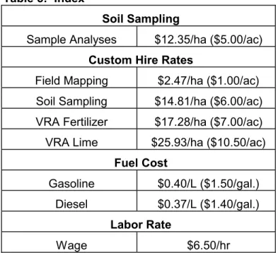
As reported by Daberkow and McBride (1999), 43% of adopters report grid sampling every four years, which is the period retained in this study. Common practices also indicate that field mapping is done every eight years, and lime applied every four years. From expert opinions, it was assumed that the annual ATV and spreader use were 800 and 1000 hours, respectively. Finally, labor cost is assumed to be $6.50 an hour and fuel cost was computed on the basis on the average of the last two years in the US and reported to be $1.50 per gallon for gasoline and $1.40 per gallon for diesel (USDA).
Analysis and Results
PA is the combination of different production operations. For the purpose of this study, these operations have been divided in four main components that will successively be investigated. The four components include: field mapping, grid soil sampling and mapping; VRA of fertilizer and VRA of lime. The focus of the study at hand is that each of these operations can be separately performed either by custom hiring, or by the farmer him/herself. Yield monitoring and variable rate seeding are not considered in this study1.
The breakeven results suggest the average American farmer would rather custom hire than buy his/her own equipment if adopting PA. The breakeven acreage for buying the PA equipment versus custom hiring is 359 ha (887 acres) while the average farm size in the United States in 2000 was 175 ha (432 acres) as shown in Table 1. Similarly, the average farm in Kentucky, (60 ha or 149 acres) would not purchase the PA equipment but rather custom hire. However, farm size estimates for row crop production in Kentucky indicate an average size of 609 ha (1504 acres) (Ibendahl and Morgan, 2000).
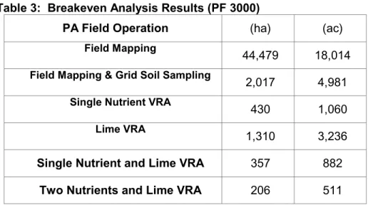
In his survey on the adoption rare of PA technology among US corn growers, Daberkow and McBride (1999) found that “soil grid sampling/mapping was the most widely used technology with 70% of farms sampling and mapping 64% of their corn acres." It is important to note that soil grid sampling and soil (or field) mapping were conjointly reported. The results in this study show that for field boundary mapping only, the minimum break-even acreage required was 18,014 ha (44,479 acres). Even if they
1 Crop yield monitoring is for many farmers the natural entry level in PA due to the maturity of the technology and the relatively low cost involved. But yield monitoring is a concentric activity with harvesting. However, custom hiring the harvest expressly to yield monitor is not a common practice. Given this, yield monitoring and yield mapping is not a PA operation wherein a farmer often chooses between custom hire or owing equipment; these PA activities are consequently not analyzed herein.
had to choose to custom hire for field mapping, current practice in Kentucky dictates that field boundary mapping is preformed free of charge when the farmer decides to grid soil sample. Thus, there is a double incentive to map boundaries and sample at the same time. The minimum acreage required to justify purchase of PA equipment for field mapping and grid sampling, combined, is 2,018 ha (4,983 acres). This result suggests that most Kentucky grain farmers would chose to custom hire this operation when field boundary mapping and soil sampling is chosen as the entry level in PA. Only the larger farms find it more profitable to invest in the equipment in such a scenario. However, it is also important to note this relatively high acreage is justified by the fact that all the PA equipment but the spreader is necessary to perform these two operations. As a result, there is a significant decrease in this break-even acreage when the spreader is added to accomplish VRA.
VRA of a single product requires the use of all the PA equipment. The break-even result found for such an application is 430 ha (1,062 acres). This result could be compared to some of the numbers reported in the Popp and Griffin (2000) survey. In this survey on early adopters in Arkansas they report that the smallest farm engaged in PA consisted of 547 ha (1350 acres) of cropped area. This suggests that all the farmers interviewed in the survey could justify investing in PA equipment for VRA of a single product. Similarly, the average commercial row crop producer in Kentucky would find it more economical to invest in its own PA equipment rather than custom hire the work. The break-even acreage for VRA decreases as more products are applied to the same ground.
Adding a VRA of lime to the mix (a single nutrient) results in a break-even acreage of 359 ha (887 acres). This decrease total in the break-even area is justified by the fact that the usage of the equipment over multiple operations reduces fixed cost. Thus, expanding the PA equipment usage to more than one product (e.g. two nutrients and lime) further lowers the break-even area to 208 ha (513 acres). However, investing in the PA equipment only to variable lime requires a minimum farm size of 1,326 ha (3,275 acres). This relatively high break-even acreage for a lime application compared to a single nutrient is not surprising as lime is typical applied at four year intervals while nutrients are applied annually. It can be concluded that the lowest number of acres that would justify that a farmer invests in PA equipment is the one where he/she would have to apply at least two nutrients and lime. Please note, the current results are applicable to the Kentucky farmer given the custom hire rate utilized in this study.
One important observation to make about this study is extreme sensitivity of the break-even area to the custom hire rate and the fixed costs. Custom hire fees are widely variable within and across regions of the US. Many factors can explain those variations. At the lower end, low PA custom hire rates can result from a fertilizer dealer marketing strategy of using VRA as a “loss leader” to bring in new clients (Lowenberg-De-Boer, 1997). Alternately, in the central cornbelt, where over half of fertilizer dealers offer VRA services, competition pushes fees down. In that area of the county where
farms are relatively bigger in size, fees are also lower because custom-hire companies can spread the fixed costs of the VRA equipment and training over more area. In regions where farm size is relatively small (as in Kentucky) custom hire fees may be relatively high as a result of little or no competition. Subsequently, a sensitivity analysis was conducted for variations of $1/ha and $2/ha for the custom rate on fertilizer and lime application. The result display in Table 4 can be summarized as follow. The sensitivity analysis shows that there is a substantial variation in the break-even acreage for change in the custom hire rate. From the highest to the lowest end the results show a variation of as much as 589 ha (1,454 acres) for lime application. In the classical case of one nutrient and lime application, the variation is almost of one to two. Finally, in the case of two nutrients and lime application an increase of the custom rate by $2 reduces the break-even area to 160 ha (395 acres). Wide variations in the break-even base line presented above are possible.
Conclusions
The results of this study suggest that the average grain producer in Kentucky should purchase PA equipment if the decision was made to adopt the technology. For the vast majority of farmers in Kentucky, not having the necessary acreage to justify the investment in PA equipment should not, however, be an obstacle not to engage in PA. As the technology matures and economic studies prove it to be profitable (Lambert and Lowenberg-DeBoer, 1994), more farmers will find it profitable to adopt the technology. Furthermore, as more farmers adopt the technology in a given region, custom hire rates will tend to go down as a result of increased competition. While lower custom hiring rates result in a higher break-even areas, the lower rates reduce the risk of experimenting with the technology for some farmers. Increased adoption will enable the technology to evolve more quickly.
Fixed costs are the most critical element of the break-even analysis. A reduction in equipment cost decreases the break-even acreage, thereby making the technology available to a wider audience of farmers. Ownership of the equipment may provide additional advantages such as better management and control of data and data generation. Ownership also enables the farmer to gain experience with PA equipment and practices, as opposed to reliance on the PA service provider or custom operator. Finally, ownership of PA equipment may facilitate its use over more operations such as variable-rate seeding, thereby spreading the fixed cost over more activities and further reducing per acre total ownership cost.
References
American Society of Agriculture Engineers. 1999. Agricultural Machinery Management Data. Agricultural Engineering Standards. pp 351-365.
Bullock, D. S., Lowenberg-DeBoer J., and S.Swinton. 2000. Assessing the Value of Precision Agricultural Data. Power Point presentation at the Spatial Analysis Learning Workshop, Berlin, August 12.
Daberkow G. and W.D. McBride. 1999. Adoption rate of site-specific crop management technologies among US corn growers. The Journal for Site-Specific Crop Management. Spring.
Doster, H. 1995. Mini-PMC user guide: Calculating machinery costs with the Purdue machinery cost calculator. C-EC-9 Rev. Purdue Univ., Dep. Agric. Econ., Coop. Ext. Serv., West Lafayette, IN
Fairchild, D. and M. Duffy. 1993. Working group report on profitability. pp 245-253. In P.C. Robert et al. (ed), Soil Specific Crop Management. ASA Misc. Publ. ASA, CSSA, Madison, WI
Kastens T.L. 2000. Precision Ag Update. Presented at: Risk and Profit 2000, Manhattan, Kansas August 17-18.
Kay R.D., Edward William M. 1999. Farm Management. Fourth edition. McGraw-Hill Book Co.
Long, D.S., G.R. Carlson, G.A Nielsen and G. Lachapelle. 1995. Increasing profitability with variable rate fertilization. Montana Ag. Research, Spring.
Lowenberg-De-Boer, J. 1994. Economics of precision farming. Ag/Innovator, Sept p 12.
Lowenberg-De-Boer, J. 1995. Management of precision agriculture data. Staff Paper 95-5, Dep. of Agric. Econ., Purdue Univ., West Lafayette, IN.
Lowenberg-De-Boer, J. 1997. What are the returns to site-specific management? In Managing Diverse Nutrient Levels: Role of Site-Specific Management: Proceedings of a Symposium Sponsored by SSSA. S-887, S-8 and A-4, Oct.27, Anaheim, CA.
Lowenberg-De-Boer, J. and M. Boehjle. 1996. Revolution, Evolution or Dead-End: Economic Perspectives on Precision Agriculture. In Proceedings of the 3rd International Conference on Precision Agriculture. ASA-CSSA-SSSA, Madison, WI June 23-26.
Lowenberg-De-Boer, J., and S.M. Swinton. 1997. Economics of Site-Specific Management in Agronomic Crops. In The State of Site-Specific Management for Agricultural Systems. F.J Pierce, P.C. Robert and J.D. Sadler, eds. Madison, WI: SSSA-CSSA. p. 369-396.
National Research Council. 1997. Precision Agriculture in the 21st Century. National Academy Press Washington, D.C.
McGill, S. 1997. Precision Farming: How to get Started. The Furrow. January.
Popp, J. and T. Griffin. 2000. Adoption, Profitability and Potential Trends of Precision Farming in Arkansas. Selected paper for the Southern Agricultural Economics Association Annual Meeting Lexington, KY, January 29-Fevruary 2.
Stombaugh T.S.and Shearer S.A. 2000. Equipment technology for precision agriculture. Journal of Soil and Water Conservation, Winter. 55(l):6.
Swinton, S.M. and Lowenberg-De-Boer, J. 1998. Evaluating the Profitability of Site-Specific Farming. In J. Prod. Agric., Vol. 11, no. 4. p 439-446
Swinton, S.M. and M. Ahmad. 1996. Returns to farmer investment in precision agriculture equipment and services. pp. 1009-1018. In Precision Agriculture. Proceedings of the 3rd International Conference, June 23-26. Minneapolis, MN. ASA-CSSA-SSSA, Madison, WI.
Zhang N., W. Maohua and W. Ning. 2001. Precision Agriculture: A Worldwide Overview. URL. http://www.bjaeu.edu.cn/keji/pc/b1.htm
Zilberman, D. 1996. Comments on Precision Agriculture. Proceedings of the Workshop on Remote Sensing for Agriculture in the 21st Century. October 23-25th.
Table 1: Fixed Costs
Equipment, Hardware & Software Function Purchase
Price Useful Life Average value Interest Depreciation OFC Fixed Total Cost
Office Computer GS1, M2,
VRA3 $1,750.00 3 $875.00 $78.75 $583.33 $4.38 $666.46
ATV M2, GS1 $5,200.00 8 $2,600.00 $234.00 $650.00 $13.00 $897.00
AgView 2.0 (VRA & Mapping) GS1, M2,
VRA3 $2,495.00 20 $1,247.50 $112.28 $124.75 $6.24 $243.26
AgView 2.0 update and support GS1, M2,
VRA3 $300.00 1 $150.00 $13.50 $300.00 -0- $313.50
PF 3000 VRA3 $4,090.00 8 $2,045.00 $184.05 $511.25 $10.23 $705.53
GPS receiver Trimble Ag 132 GS1, M2,
VRA3 $3,400.00 5 $1,700.00 $153.00 $680.00 $8.50 $841.50
Differential correction subscription GS1, M2,
VRA3 $800.00 1 $400.00 $36.00 $800.00 $0.00 $836.00 PC card reader GS1, M2, VRA3 $200.00 3 $100.00 $9.00 $66.67 $0.50 $76.17 Spreader VRA3 $10,000.00 5 $5,000.00 $450.00 $2,000.00 $125.0 0 $2575.00
VR Controler : Rawson Controler VRA3 $3,300.00 8 $1,650.00 $148.50 $412.50 $8.25 $569.25
Total $31,535.00 $15,767.50 $1,419.08 $6,128.50 $176.0 9
$7,723.66
1. GS: Grid Sampling
2. M: Mapping and Recommendation 3. VRA: Variable Rate Application
Table 2: Variable Costs
Function Use. (hr) Perform. Rate (ac/Hr) Fuel Factor R&M Factor Repairs & Maint. Fuel, Oil & Lube Labor Total Variable Costs ATV
Soil sampling 800 45.00 0.50 0.50 0.018 0.005 0.036 $0.059/ac
Field boundary mapping M1, GS2
800 60.00 0.50 0.50 0.007 0.002 0.014 $0.022/ac
Spreader
Single nutrient application 1000 61.091 8.081 2 0.327 0.213 0.106 $0.647/ac
Lime application VRA3
1000 8.333 8.081 2 0.600 0.390 0.195 $1.185/ac
Total $1.913/ac 1. M: Mapping and Recommendation
2. GS: Grid Sampling
Table 3: Breakeven Analysis Results (PF 3000)
PA Field Operation (ha) (ac)
Field Mapping
44,479 18,014
Field Mapping & Grid Soil Sampling
2,017 4,981
Single Nutrient VRA
430 1,060
Lime VRA
1,310 3,236
Single Nutrient and Lime VRA 357 882
Two Nutrients and Lime VRA 206 511
Table 4: Sensitivity Analysis
Application Practice + $2 + $1 - $2 -$1
Single Nutrient 337 ha (833 ac) 378 ha (934 ac) 500 ha (1231 ac) 593 ha (1465 ac) Single Nutrient
and Lime
279 ha (689 ac) 314 ha (775 ac) 419 ha (1035 ac) 503 ha (1243 ac) Two Nutrients
and Lime
160 ha (395 ac) 180 ha (446 ac) 244 ha (603 ac) 296 ha (731 ac) Lime 1,095 ha (2702 ac 1,199 ha (2961 ac) 1,484 ha (3663 ac) 1,684 ha (4156 ac)
Table 5: Index
Soil Sampling
Sample Analyses $12.35/ha ($5.00/ac) Custom Hire Rates
Field Mapping $2.47/ha ($1.00/ac) Soil Sampling $14.81/ha ($6.00/ac) VRA Fertilizer $17.28/ha ($7.00/ac)
VRA Lime $25.93/ha ($10.50/ac)
Fuel Cost
Gasoline $0.40/L ($1.50/gal.)
Diesel $0.37/L ($1.40/gal.)
Labor Rate