UC Davis
Electrical & Computer Engineering
Title
Dynamic Graphs on the GPU
Permalink
https://escholarship.org/uc/item/48j4k7np
Authors
Awad, Muhammad A.
Ashkiani, Saman
Porumbescu, Serban D.
et al.
Publication Date
2020-05-01
Peer reviewed
eScholarship.org
Powered by the California Digital Library
Dynamic Graphs on the GPU
Muhammad A. Awad
Dept. of Elect. & ComputerEngineering, UC Davis Davis, California, USA [email protected]
Saman Ashkiani
† Dept. of Elect. & ComputerEngineering, UC Davis Davis, California, USA [email protected]
Serban D. Porumbescu
Dept. of Elect. & ComputerEngineering, UC Davis Davis, California, USA [email protected]
John D. Owens
Dept. of Elect. & ComputerEngineering, UC Davis Davis, California, USA [email protected]
Abstract—We present a fast dynamic graph data structure for the GPU. Our dynamic graph structure uses one hash table per vertex to store adjacency lists and achieves 3.4–14.8x faster insertion rates over the state of the art across a diverse set of large datasets, as well as deletion speedups up to 7.8x. The data structure supports queries and dynamic updates through both edge and vertex insertion and deletion. In addition, we define a comprehensive evaluation strategy based on operations, workloads, and applications that we believe better characterize and evaluate dynamic graph data structures.
Index Terms—dynamic, graph, data structures, GPU I. INTRODUCTION
While interest in graph analytics on GPUs has exploded in recent years, the vast majority of this work focuses on static graphs that never change during the graph computation. To-day’s GPU graph analytic frameworks generally lack a GPU-managed dynamic graph data structure that supports changes (insertions and deletions) to the graph as well as queries into this data structure. The key challenge is representing the neighbors of each vertex (the “adjacency list”), where that data structure must be flexible enough to support a wide range of sizes and efficiently allow both queries into and changes to this data structure.
Previous efforts to support GPU-based dynamic graph data structures represent an adjacency list with a list-based data structure [1, 2] or an array-based data structure that maintains sort order [3]. Its implementation as a list/array presents a dilemma for its designer:
• Adjacencies can be stored as an unsorted list, which is easy to maintain. However, unsorted lists are unaccept-ably slow for important operations on the data structure, e.g., edge-existence queries (“doesv haveuas a neigh-bor”) or insertions that do not result in duplicates, both of which require traversing the entire list. Consequently, with an unsorted list, many operations are O(n) in the size of the list. This cost is prohibitive for vertices with many neighbors, as is common in scale-free graphs. • To eliminate thisO(n)cost, the adjacencies can instead
be stored as a sorted list. These expensive operations become O(logn)in the size of the list, but now the data structure must maintain the list in sorted order, which incurs a significant cost.
†Currently works at OmniSci, Inc.
From a performance standpoint, neither alternative is ac-ceptable. Now, some graph operations can be implemented with high performance on an unsorted list, and thus for a subset of graph workloads, a list-based data structure may deliver acceptable performance. But many graph operations cannot be implemented without paying the high cost of a full search of an unordered list or the maintenance cost of preserving sorted order.
We believe that existing dynamic GPU graph data structures like faimGraph [2] and Hornet [1] are suboptimal when con-sidering real-world dynamic graph scenarios. Truly dynamic data structures need to support continuous modifications not only from running the algorithm (e.g., edge deletion in k-truss), but also from a flowing stream of edge and vertex insertions and deletions. While a reasonable first step, the experiments presented in the faimGraph and Hornet works lack the true dynamism we expect in real world scenarios. Their chosen approaches both rely heavily on potentially expensive sorting operations necessary for vertex and edge deduplication. In general, duplicate entries lead to incorrect graph analytic results for the many graph primitives where idempotence does not apply (e.g., triangle counting or betweenness centrality).
We show that using a more sophisticated data structure (e.g., a hash table), we achieve better performance compared to list-based techniques provided by alternative data structures (e.g., faimGraph or Hornet). A major reason for our superior performance is the fast query rates that hash tables offer and their ability to ensure uniqueness while performing updates. In contrast, list-based data structures require explicit sorting for deduplication to maintain uniqueness. To evaluate our data structure, we integrate it into the Gunrock GPU graph analytics framework [4] and compare it against other dynamic graph data structures. The resulting overall performance of our data structure on a range of workloads and applications, particularly on insertions, is superior to existing alternatives and also allows reasonable tradeoffs dependent on the selected workload.
Our contributions in this work are:
1) A high-performance hash table based dynamic graph data structure that supports extremely high rates of insertions and deletions (sections III and IV);
2) An evaluation strategy that defines a set of workloads to benchmark a dynamic graph data structure (section V); and
3) Exploring the use of a dynamic graph data structure in applications while maintaining an updated graph (section VI).
II. BACKGROUND ANDPREVIOUSWORK A. Background
Consider a directed weighted graphG= (V,E,W)1, where
V, E, and W represent the vertex set, edge set, and edge weight set respectively. For each arbitrary vertex u ∈ V, we represent its outgoing neighbors (adjacency list) with Au. e = hu, v, wi ∈ E represents an edge from vertex u∈ V to
v∈ V with weight w.
It is common to use an adjacency matrix with|V|2elements
to represent dense graphs. Updating an adjacency matrix is trivial. However, ifG is a sparse graph (i.e.,|E| |V|2), then
the adjacency matrix is largely empty and, in practice, requires far too much memory for large graphs. Several alternative sparse graph representations exist. For example, Compressed Sparse Row (CSR), Compressed Sparse Column (CSC), and Coordinate list(COO) all offer better memory efficiency than the equivalent sparse adjacency matrix.
In CSR, for instance, Au is stored as an array of values
(weights) and an array of destination vertex IDs. Then all adjacency lists (arrays of size equal to the out-degree of each vertex du, where Pu∈Vdu =|E|) are concatenated to form
two large arrays of size|E|. A ternary array (i.e., row pointers) marks the start and end index of each adjacency list (i.e., each vertex’s neighbors). CSR’s representation requiresO(|E|+|V|) elements, which is considerably more memory efficient than the O(V2) required for adjacency matrix. However, since it
is a packed data structure, it is not possible to update it (i.e., delete or insert a new edge or vertex) without rebuilding the entire data structure.
In this work, we design a graph data structure that is both memory-efficient (like CSR) and also update-friendly (like the adjacency matrix). Suppose Au represents the adjacency list
of a particular vertex u∈ V, whereAu contains destinations
of all outbound edges connected tou. Then a dynamic graph data structure should support the following operations:
1) Retrieving the adjacency list of vertexu: returnsAu if it
exists,⊥otherwise.
2) Inserting a new vertex u: Insert(u), whereAu is
initial-ized with all connected vertices to u.
3) Deleting a vertex u: Delete(u), whereAu can no longer
be located. Au is deleted. All edges that haveuas their
destination should be removed either immediately or in a lazy fashion. After a deletion, no edge query involving
umay have a false positive result. QueryingAu returns
no edges.
4) Inserting a new edge: Insert(hu, v, wi), whereAu is first
located, then a new pair hv, wiis inserted intoAu.
1In general, we would like to support arbitrary meta-data assigned to each
vertex or edge (DV andDE). Here, for the sake of clarity, we assumeW
represents any sort of meta-data associated with vertices or edges.
5) Deleting an edge: Delete(hu, v, wi), where Au is first
located and then the pairhv, wiis deleted.2
We assume that for each vertex u∈ V, the adjacency list
Au is stored in a data structure that supports the following
three operations:
1) SearchAu(v): search through adjacency list Au and
re-turnshv, wiif present, ⊥otherwise.
2) InsertAuhv, wi: inserts a new entry hv, wiinto the
adja-cency listAu.3
3) DeleteAu(v): delete any entrieshv, wifrom the adjacency
listAu.
In general we assume that all of the operations are batched and performed in a phase-concurrent fashion (i.e., updating the data structure does not happen concurrently with any kind of read-only search query from the data structure).
B. Previous Work
The major challenge for an efficient dynamic graph data structure on the GPU is the design of the adjacency list data structure to best accommodate potential updates. Memory management of this data structure is inherent in this challenge. Sha et al. proposed GPMA as a GPU-friendly data structure for dynamic graphs [3] based on the Packed Memory Array data structure (PMA) [5]. PMA is a kind of balanced binary search tree, where nodes are sorted arrays with some anticipated empty gaps to support potential updates. PMA uses lower and upper bound density thresholds for each node, and these thresholds are used to make decisions to either copy a node into a larger newly allocated node (high density), or properly merge multiple nodes into a single node (low density). In GPMA, a batch of updates is first sorted. The sorted batch is further partitioned into several continuous parts, where each part will only belong to a single node in the tree. Then each node is properly updated based on its partition’s size in three granularities of warp/block/device. Sha et al. proposed a method to store a CSR format for a graph in a GPMA data structure. There is little discussion of memory management. Most of the experiments on updating the data structure are around edge insertions, but lazy edge deletions are also briefly discussed.
Hornet [1] divides the allocated available memory into blocks that can store a number of edges up to a specific power of two. Initially an adjacency list is stored inside the smallest power-of-two memory block that can contain it. During edge insertion, if the newly inserted edges exceed the capacity of a memory block, the vertex adjacency list is copied to the next smallest power-of-two memory block. For each array of blocks, a B-Tree tracks the free and used ones. Memory management is done on the CPU. Hornet achieves a compact representation for an adjacency list at the expense of
2One can define more general edge deletion operations such that all
instances ofhu, v,·i are deleted regardless of their weights. This version might be useful if we allow multiple edges from a source to a destination, each with a different weight or meta-data.
3Duplicates are not allowed: first search for v (i.e., search
Au(v)), and
memory fragmentation. Moreover, it supports vertex insertion (or deletion) through a series of corresponding edge insertions (or deletions).
faimGraph [2] uses a single memory pool on the GPU for both the data structure and the algorithm that solves a graph problem. In contrast to Hornet, faimGraph’s memory management is entirely on the GPU. Queues are used for memory reclamations of pages and deleted vertex IDs. faim-Graph maintains a mapping between vertex IDs on the GPU and CPU. It also offers both structure-of-arrays (SoA) and array-of-structures (AoS) representations to store edge data, where the former is used for edges with a single property and the latter is used for edges with multiple properties. Memory pages configurable in size contain pointers to next pages when the adjacency list size exceeds a single page size. Using different GPU and CPU vertex IDs allows for flexible memory reclamation.
Edge duplication is not allowed in either Hornet or faim-Graph. Both take preventive measures during updates to ensure edge uniqueness in the data structure.
We discuss and compare our results to faimGraph and Hornet. faimGraph is the state-of-the-art dynamic graph data structure and Hornet is a maintained graph processing library. In terms of similarities, our work is similar to faimGraph as our hash table is represented using fixed-size memory pages. In other words, if the hash table consists of a single bucket, which is true in road-network-like graphs (but not scale-free graphs), our work and faimGraph are similar. Similar to Hornet, addition of new vertices in our system requires overallocation of the graph data structure capacity to avoid reallocation, but we keep in mind that the cost of reallocation only requires copying of adjacency-list pointers and not the entire data structure.
III. OURGPU DYNAMICGRAPH
The key challenge in designing a dynamic graph data structure is storing per-vertex adjacency lists. Our graph representation uses a separate data structure for each vertex adjacency list together with associated handles to reach those adjacency lists as necessary to perform various operations. The choice of the data structure used to store adjacency lists must be based on tradeoffs between what operations the data structure supports, the performance of individual operations, and the requirements of the graph library for solving specific problems. For instance, the simplest data structure choice is to use a variable-sized list data structure per adjacency list, with the designer either choosing to keep that list unsorted or maintain it as a sorted list. Hornet [1] embodies this approach. This representation is the most compact, but incurs a large maintenance overhead when compared to other options. Another possibility is the approach taken by faimGraph [2], which relaxes the variable-sized list constraint and instead breaks lists into fixed-size pages to simplify the maintenance of the data structure. Our position is that these primitive GPU data structures can be replaced by more sophisticated ones such as hash tables [6] or B-Trees [7], depending on the
requirements of the problem in terms of the performance and availability of data structure operations. In this work our goal is to provide a high throughput of both updates and lookups, thus we pick hash tables.
Advantages of a hash table representation: The primary advantage of hash tables is their efficient operations (both mutations and queries). Supporting efficient queries is an essential requirement in a graph data structure. Not only do graph applications perform read-only queries into graphs, but even mutation operations typically incorporate queries. For instance, an insertion while maintaining unique edges first requires a query determining whether the edge exists or not, followed by the insertion process itself (this is simply writing the new pair into an empty location). For a list-based data structure, performing a query operation is eitherO(n)(for an unsorted list) orO(logn)(for a sorted list) in the size of the list. For a hash table with a suitable load factor, queries are instead O(1). In a dynamic setting, hash table performance can decrease as the chain-length increases (i.e., load factor increases). In practice we can maintain low-cost metrics per vertex to determine the chain-length and periodically perform rehashing if it exceeds a given threshold.
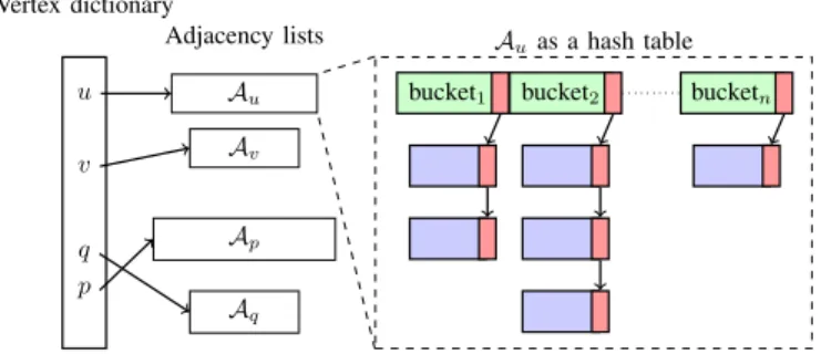
Fig. 1 shows a high-level representation of our graph data structure, which is divided into two parts:
a) Vertex dictionary: We store vertices, V, in a simple fixed-size array, indexed by vertex ID. The array size can be increased if needed, but frequent reallocation should be avoided to minimize the performance costs commonly associ-ated with memory allocation. Selecting a large-enough initial capacity based on graph problem requirements ensures good performance during vertices insertion.
b) Adjacency lists: We use one hash table per vertex to store its associated adjacency list Au. Given a load factor
and number of edges in an adjacency list, we calculate the number of buckets in a hash table. Note that the load factor, directly related to the number of buckets, provides a tradeoff between two main operations: 1) reading a complete adjacency list associated with a vertex and 2) performing an edge-exists query in a vertex’s adjacency list. In practice we select a single load factor for all hash tables (in this work, we use a load factor of 0.7). This is not strictly necessary, but determining an ideal load factor per-vertex (per-hash-table) a priori is difficult. Our dynamic graph data structure can make use of given connectivity information along with the choice of the load factor to determine the number of necessary buckets to allocate. This decision results in significant performance gains by reducing memory allocation overhead. Using a dynamic memory allocator, any hash table can dynamically allocate additional slabs as needed (Fig. 1). If the connectivity infor-mation for a vertex is not available, we construct a hash table with a single bucket for this vertex.
IV. IMPLEMENTATION
Our dynamic graph data structure’s adjacency lists are stored as hash tables. In this work, we use Slab Hash, a dynamic hash table data structure for the GPU [6], as the basis
Vertex dictionary u Au Adjacency lists v Av p Ap q Aq Auas a hash table bucket1 bucket2 bucketn
Fig. 1: High level schematic of our graph data structure. Each adjacency list is represented using a slab hash. The number of base slabs per adjacency list depends on the load factor used per adjacency list. Base slabs are statically allocated in consecutive memory locations, while the slabs used to re-solve collisions are allocated dynamically and reached through pointers.
of our underlying hash tables.4We have significantly improved the functionality of the original slab hash in order to meet our requirements.5 We offer two variants of our dynamic graph
data structure. One uses Slab Hash’s concurrent map, which should be used if storing a value per edge is required. The second variant uses Slab Hash’s new concurrent set, which should be used if edge values are not required. Any hash table design can be used for this underlying data structure, as long as it is efficient in both searching (for queries) and updating the data structure itself (for insertions and deletions). In the end, the performance of our graph data structure directly depends on the performance of its underlying hash tables.
We integrate our dynamic graph data structure into the Gunrock GPU graph analytics framework [4]. In order to take advantage of the high-performance operations Slab Hash offers, all our operations are implemented based on the Warp Cooperative Work Sharing (WCWS) strategy [6]. In WCWS, each thread has an independent task assigned to it, but all threads within a warp cooperate with each other to collectively perform one independent task at a time. This is the right design decision because it better matches the memory access pattern desired by the GPU hardware (coalesced memory accesses), and hence it provides better performance for updates. On the downside, it requires all threads within a warp to be active. In other words, an operation on the data structure can not be performed within a branch where threads (in a warp) diverge when executing it.
A. Memory Management
Our memory management is divided into two parts: 1) vertex dictionary memory, and 2) hash table memory.
4https://github.com/owensgroup/SlabHash
5The original slab hash only provided aconcurrent map data structure,
without any restrictions on duplicate keys. To name a few of our recent additions: maintaining key-uniqueness, proper iterator access, and design and implementation of a new concurrent set (keys only, and no values).
1) Vertex dictionary memory: Defining a graph requires defining the graph’s vertex capacity. The vertex dictionary stores pointers to the hash table associated with each vertex’s adjacency list. When inserting more vertices than the vertex dictionary’s capacity, we copy the vertex dictionary to a new memory location after increasing its capacity. This process only requires shallow copying of the pointers to each of the hash tables (including pointers to the hash tables associated with the new vertices).
2) Adjacency list hash table memory management: Con-structing a hash table requires choosing and allocating a number of buckets (base slabs) that are required for insertion processes. The initial number of buckets for a vertex u is
d|Au|/(lf×Bc)e, where lf is the load factor and Bc, the
bucket capacity per slab, is either 15 or 30 for Slab Hash map or set, respectively. During insertion, if a bucket’s slab becomes full (capacity achieved), Slab Hash dynamically allocates a new slab for that bucket that is singly linked to the tail of the list; a dynamic memory allocator handles these dynamic allocations [6]. Only when we perform vertex deletion (essentially this deletes an entire hash table) do we free this dynamically allocated memory (Section IV-D2).
Our graph data structure handles the memory allocation required for the initial buckets by statically allocating all the memory required for the initial buckets in bulk. This is more desirable than requiring each hash table to independently allo-cate a small number of buckets with differentcudaMalloc
calls. We initialize a vertex’s hash table with its initial number of buckets, the memory address for its first bucket, and the number of neighbors (to zero). In cases where the number of neighbors is not defined, we allocate a single bucket. B. Query operations
To iterate over a vertex’s adjacency list, we provide a vertex adjacency list iterator. For a given vertex, the iterator loops over all of the hash table buckets associated with the vertex as well as additional slabs used to resolve hash collisions. The iterator loads one slab at a time and moves from one slab to the next using a nextoperator.
We also provide an edgeExistquery that checks if the destination v of a given pair hu, vi exists in the hash table associated with u. edgeExist simply performs a search query [6] inu’s hash table.
C. Edge operations
We interpret edge operations (insertion and deletion) as modifications to the source vertex’s adjacency list. As dis-cussed in Sec. III, we use a hash table to represent each vertex’s adjacency list. We discuss this in more depth below in the context of a directed graph. In an undirected graph, in-serting (or deleting) an edge between a source and destination is similar but also requires an operation on the edge in the other direction. Our semantics for edge operations follows the semantics for hash table operations, which we discuss below.
1) Edge insertion: Algorithm 1 shows high-level pseu-docode for an edge insertion. We assume that each thread has a single edge to insert. Initially, in Line 3, we ensure no self-edges are allowed. A work queue is constructed within a warp (Line 4) through a ballot instruction on all threads’ remaining tasks. All threads locate the next task to perform (through finding the first set bit in the work queue as in Line 5) and then get the corresponding source vertex of the chosen task (through a shuffle instruction as in Line 6). Since multiple edges within a warp might share the same source vertex (Lines 7 and 8), all these insertions are grouped together to be performed in one single coalesced call to the hash table associated with the source vertex. We implemented and used a new slab-hash replace operation to ensure key-uniqueness in the hash table (i.e., unique destination vertices). In this operation, if a key (a destination vertex) already exists in the hash table, it will be replaced with the most recent value. Otherwise, a new key-value pair is added to the hash table. If the batch of edges contains the same unique edge but with different weights, only the most recent edge and its weight will be stored in the graph. The replace operation returns a boolean value indicating whether a new key (i.e., an edge) was added to the hash table or the key previously existed and was hence just replaced. We use this returned boolean variable to maintain an exact number of edges per vertex (population count on all successful additions within a warp in Line 10). The thread whose task was just completed, as well as all threads that shared the same source vertex (i.e., the coalesced insertion group), mark themselves as completed (Line 11). We repeat this procedure until the work queue is completely empty, i.e., no more edges remain to be inserted.
2) Edge deletion: Edge deletion is similar to edge insertion with two major differences: 1) instead of using the replace operation in Algorithm 1, we use the delete operation; 2) the delete operation also returns a boolean variable as to whether the key already existed. This boolean variable is used to decrement the number of edges that belongs to the adjacency list of the vertex. Note that in order to maintain uniqueness within the slab hash (due to how insertion/replace operations are designed and implemented), deleted edges (i.e., keys) are only marked as deleted (i.e., by replacing a key with a tombstone) and not explicitly removed. Tombstones are disregarded in edge insertion (as if that particular location is not empty). Tombstones can later be completely flushed out of the data structure, if required. Together, these design decisions ensure that empty locations can only exist at the end of each bucket’s list in the slab hash. Moreover, not overwriting tombstones results in faster insertion rates (since new edges are only added to the end of the bucket’s linked list). This comes at the expense of having unused memory locations. A different approach would be to break down the insertion process into two stages: 1) traversing the bucket’s linked list to ensure uniqueness, then 2) for unique keys, a follow-up insertion that overwrites tombstones. We use the former approach during insertions, but the latter could be used to optimize for memory usage on the expense of decreased
insertion throughput. D. Vertex Operations
1) Vertex insertion: We define a vertex insertion operation as the operation of inserting edges connected to a vertex that has an empty adjacency list. As discussed earlier, if the new vertex count exceeds the capacity of the vertex dictionary, we first extend the vertex dictionary. Once the vertex is entered into the dictionary, we then insert all attached edges using Algorithm 1.
2) Vertex deletion: Algorithm 2 summarizes this process for an undirected graph. Each warp deletes one vertex at a time. Because each vertex in a multi-vertex deletion operation may have a different number of edges, a straightforward implementation would suffer from load imbalance. We address this imbalance with a simple technique. We maintain a queue of deleted vertices with an atomic counter (Line 4). A single thread inside the warp acquires a new vertex from the queue (Line 3). The new vertex queue location is broadcast for all threads in the warp (Line 6). The vertex-deletion kernel only exits after deleting all the required vertices (Line 8). A warp reads the vertex index (Line 10) and requests an edge iterator over the all the slabs associated with the vertex (Line 11). Using the iterator, we loop over all of the vertex destinations and delete the vertex from their adjacency lists (Line 16). Additionally, all dynamically allocated memory (i.e., memory used to resolve collisions) is freed and reclaimed by the memory allocator (Line 19). Finally, the count of edges connected to the vertex is set to zero (Line 22). Statically allocated memory is not reclaimed. For a directed graph, the only requirement is to free the memory. To clean up, we end with a follow-up lookup and delete all of the deleted vertices in all of the hash tables.
Algorithm 1 Graph edge insertion algorithm. 1: procedureINSERTEDGES(GpuGraph graph, Edges edges)
2: thread edge←edges[threadIdx]
3: to insert←thread edge.src != thread edge.dst
4: whilework queue←ballot(to insert)do 5: current lane←find first set bit(work queue)
6: current src←shuffle(thread edge.src, current lane)
7: same src←thread edge.src == current src
8: success←graph[current src].replace(thread edge, same src & to insert)
9: added count←popc(ballot(success))
10: graph[current src].incrementEdgesCount(added count)
11: ifsame src & to insertthen 12: to insert←false
13: end if 14: end while 15:end procedure
V. EVALUATIONSTRATEGY
Our community has not yet defined consistent standards for evaluating a dynamic graph data structure. In part this is because of the very recent development of these data structures as a topic for study. As a result, we lack a broad set of appli-cations or workloads that require dynamic data structures. We believe the evaluation we present below improves on previous work by identifying and characterizing a set of operations, workloads, and applications that together encompass the wide
Algorithm 2 Graph vertex deletion algorithm.
1:procedure DELETEVERTICES(GpuGraph graph, Vertices vertices, Count count, Queue queue) 2: while true do 3: iflaneId == 0then 4: queueId←atomicAdd(queue, 1) 5: end if 6: queueId←shuffle(queueId, 0)
7: ifqueueId≥countthen 8: return
9: end if
10: warp vertex←vertices[queueId]
11: vertex edges it←GpuGraph::EdgeIterator(warp vertex)
12: whilevertex edges it.next()do
13: lane dst←vertex edges it.getDst(laneId)
14: forlane in lanesdo
15: current dst←shuffle(lane dst, lane)
16: graph[current dst].delete(warp vertex)
17: end for
18: ifvertex edges it.current() is not base slabthen 19: free(vertex edges it.getAddress())
20: end if 21: end while
22: graph[warp vertex].setEdgesCount(0)
23: end while 24: end procedure
range of use cases that will be addressed with dynamic graph data structures.
We believe a comprehensive evaluation requires three com-ponents:
Operations Dynamic data structures support particular oper-ations, e.g., edge and vertex deletion and insertion. We enumerate these operations and measure their throughput.
Workloads Because dynamic graph data structures on the GPU are not yet in significant use, applications that use them are few. However, we present a set of workloads— common patterns of how we will use the data structure— that we believe will underlie future applications in this area.
Applications Finally, prior work has identified particular ap-plications on which they evaluate their data structure. We evaluate our work on these specific applications as well. A. Low-Level Operations on a Dynamic Graph Data Structure We begin with measuring throughput for the important low-level operations on our data structure:
1) Edge Insertion and Deletion: Starting from a static graph stored in a dynamic data structure, we measure the throughput of edge insertion and deletion operations for differ-ent batch sizes. Edges are inserted or deleted between existing vertices in the graph. Duplicate edges are allowed within a batch and across the batch and the graph. The graph data structure only maintains unique edges.
2) Vertex Insertion and Deletion: Similar to edge insertion and deletion, we start from a static graph and measure the throughput of inserting and deleting vertices in different batch sizes.
B. Workloads on a Dynamic Graph Data Structure
To evaluate a dynamic graph data structure we propose the following different set of workloads. Each one of these workloads targets a different scenario, not specific to any
particular application, that we expect to be a pattern that can be used in real-world applications.
1) Static Workloads / Bulk-build: We start by comparing our dynamic graph data structure to other alternatives in a static setting. Specifically, we evaluate the performance of building a static graph. We assume that the number of edges per vertex and the number of vertices is known a priori.
Given a static graph, we measure the time required for building the graph in bulk and compare this with previous work. We assume that the input is given in a COO format (i.e., a list of edges each defined by source vertex, destination vertex, and edge value).
2) Dynamic Workloads / Incremental Build: Starting with an empty graph, we incrementally build a graph using different batch sizes. In general, to avoid memory reallocation we assume that a suitable vertex capacity (i.e., maximum number of vertices) is known.
C. Applications with a Dynamic Graph Data Structure We again emphasize that the existing set of graph appli-cations that use dynamic data structures is small. We thus primarily evaluate work on the applications developed in and described by previous work where possible. For the static application case, we use static triangle counting to evaluate and compare our dynamic graph data structure performance to static CSR [4] and the two dynamic graph representa-tions [1, 2]. In the dynamic application case, we evaluate based on a dynamic triangle counting application that performs triangle counting after each batch insertion. Note that in this work we only focus on the performance of the dynamic graph data structure. Optimizing a static or dynamic graph algorithm (e.g., triangle counting) is beyond the scope of this paper.
VI. RESULTS
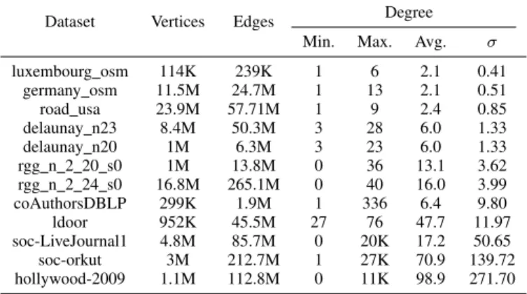
We evaluate and compare our dynamic graph data structure to Hornet6 and faimGraph7. faimGraph is the state of the art in dynamic GPU graph data structures. Hornet is an actively maintained GPU data structure for sparse graphs and matrices. In our tests, faimGraph’s page size is configured to be 128 bytes to match our slab page size. Our tests do not require that either faimGraph or Hornet maintain a sorted adjacency list. All of our measured performance timings for all libraries only include the time to perform the operation and do not include the time required to transfer memory between CPU and GPU. We perform our benchmarking using the datasets shown in Table I on an NVIDIA TITAN V (Volta) GPU with 12 GB DRAM and an Intel Xeon CPU E5-2637.
A. Operations
1) Batched Edge Insertion: We perform a batched edge insertion (Sec. V-A1) for different batch sizes and measure the average throughput for all the given datasets. faimGraph only supports batch updates of sizes less than 1M. Table II
6https://github.com/hornet-gt/hornet/tree/a5c754d9616f54404a7b2a15c11143d52a346ab9 7https://bitbucket.org/mwinter92/faimgraph
TABLE I: Datasets
Dataset Vertices Edges Degree Min. Max. Avg. σ
luxembourg osm 114K 239K 1 6 2.1 0.41 germany osm 11.5M 24.7M 1 13 2.1 0.51 road usa 23.9M 57.71M 1 9 2.4 0.85 delaunay n23 8.4M 50.3M 3 28 6.0 1.33 delaunay n20 1M 6.3M 3 23 6.0 1.33 rgg n 2 20 s0 1M 13.8M 0 36 13.1 3.62 rgg n 2 24 s0 16.8M 265.1M 0 40 16.0 3.99 coAuthorsDBLP 299K 1.9M 1 336 6.4 9.80 ldoor 952K 45.5M 27 76 47.7 11.97 soc-LiveJournal1 4.8M 85.7M 0 20K 17.2 50.65 soc-orkut 3M 212.7M 1 27K 70.9 139.72 hollywood-2009 1.1M 112.8M 0 11K 98.9 271.70
TABLE II: Mean edge insertion rates (in MEdge/s) for differ-ent batch sizes.
Batch size Hornet faimGraph Ours
216 33.67 92.47 501.33 217 44.71 133.97 513.56 218 51.43 157.15 591.06 219 70.81 188.98 641.25 220 83.54 — 664.52 221 97.41 — 658.09 222 110.89 — 646.01
compares our edge insertion throughput to Hornet and faim-Graph. Our speedup ranges between 5.8–14.8x compared to Hornet and 3.4–5.4x compared to faimGraph.
2) Batched Edge Deletion: Similar to batched edge inser-tion, we run a batched edge deletion. Table III shows the result of this benchmark. This is where Hornet performance becomes competitive with ours. Deletion is a simple process and does not require cross-duplicate checking between the graph and the input batch. Note that for small datasets, the true number of deleted edges (i.e., unique edges within the batch) is much lower than the number of randomly generated edges, hence resulting in less work in general. Our performance is as fast as Hornet for a large batch size and almost 7x faster for a smaller batch size of216. Our deletion rates are between 3.6–
7.8x faster than faimGraph’s.
TABLE III: Mean edge deletion rates (in MEdge/s) for differ-ent batch sizes.
Batch size Hornet faimGraph Ours
216 91.73 111.71 640.63 217 159.69 112.96 886.92 218 259.31 171.75 947.60 219 377.79 257.66 939.98 220 537.73 — 988.85 221 739.82 — 1,007.16 222 1,024.87 — 1,015.47
TABLE IV: Mean vertex deletion throughput (in MVertex/s) for different batch sizes.
Batch size faimGraph Ours
216 0.44 5.35
217 0.71 9.23
218 1.12 12.66
219 1.62 19.21
220 2.96 26.49
3) Vertex Deletion: Beginning with an undirected graph, we delete a batch of vertices and measure the throughput of vertex deletion. Table IV shows the throughput for dif-ferent batch sizes averaged over four datasets: orkut, soc-LiveJournal1, delaunay n23, and germany osm. Our vertex deletion throughput is between 8.9–12.2x faster than faim-Graph (Hornet does not implement vertex deletion). Both we and faimGraph delete vertices from neighbor adjacency lists and free the memory used to store the vertex adjacency list, but faimGraph implements one operation that we do not: it places the deleted vertex into a vertex queue and can thus reuse identifiers of deleted vertices during subsequent vertex insertions. This allows faimGraph to be more memory efficient compared to our approach. It would be straightforward to implement the same strategy with our data structure but we have not yet done so. If we compare only delete and free operations common to both data structures, our speedup is 8.5–11.56x over faimGraph. As with query operations, the dominant factor in vertex-deletion performance is looking up a deleted vertex in its neighbors’ adjacency lists; this is faster in a hash table than in a list.
B. Workloads
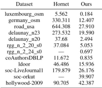
1) Bulk Build: We perform the bulk build benchmark from Sec. V-B1. Bulk build is simply inserting all edges from a graph into the graph data structure in one single batch. We implemented the bulk build functionality in Hornet only. Table V shows the time required to bulk build the datasets. For two datasets—rgg n 2 24 s0 and soc-orkut—Hornet runs out of memory. We believe that this is due to the memory overhead of sorting and duplicate checking. Our dynamic graph data structure is 2–30x faster. Note that for a large dataset, hollywood-2009, 45% of Hornet’s insertion time is spent in duplication checking alone, which is the same time as our entire build.
2) Incremental Build: In this benchmark we begin with an empty graph and incrementally insert edges (Sec. V-B2). The goal is to test and measure the edge throughput when building a graph data structure given a known bound on the number of vertices a priori, but an unknown number of edges. For our dynamic graph data structure, this means that each hash table is given only one bucket (i.e., a single linked list). Note that in this experiment our data structure is similar to faimGraph, but differs from Hornet in our use of a linked list of pages versus a single block containing the adjacency list. For our
TABLE V: Bulk build elapsed time (ms). Dataset Hornet Ours luxembourg osm 5.562 0.184 germany osm 330.311 12.407 road usa 644.308 27.910 delaunay n23 273.532 19.590 delaunay n20 37.68 2.494 rgg n 2 20 s0 37.084 5.053 rgg n 2 24 s0 — 0.697 coAuthorsDBLP 11.672 0.835 ldoor 46.486 15.936 soc-LiveJournal1 179.879 26.176 soc-orkut — 39.907 hollywood-2009 90.705 42.387
TABLE VI: Incremental build mean edge insertion rates (in MEdge/s) for different batch sizes.
Batch size Hornet Ours
220 164.44 841.31
221 176.96 945.64
222 184.75 993.82
hash table based graph data structure, this represents the worst-case scenario.
Table VI shows the average throughput for building graphs with a similar number of edges (ldoor, delaunay n23, road usa, soc-LiveJournal1) using different batch sizes. We implemented incremental build in Hornet only. On average our data structure is 5x faster than Hornet. For the two low-variance graph datasets (delaunay n23 and road usa), our speedups are between 15–25x. We believe that the main reason for our performance advantage is that Hornet maintains its adjacency list in a single fixed-size block. When an added edge exceeds the size of the block, the entire adjacency list must be copied to an existing or newly allocated empty block of the appropriate size. In contrast, our linked lists avoid copying and simply allocate new pages to accommodate new edges as needed. With Hornet, copying into larger-sized blocks is expected to happen more often for low-variance datasets. For high-variance datasets, Hornet’s doubling adjacency list strategy becomes more efficient because the need for copying to new blocks decreases. We see speedups of 1.6–2.5x for the ldoor dataset, but for the soc-LiveJournal1 dataset our throughput is 0.92x slower.
C. Applications
We pick triangle counting as a simple application to explore the interaction between a dynamic data structure and solving a graph problem. Our goal here is not to provide an optimal solution to the dynamic triangle counting problem; rather, we would like to explore the performance of triangle counting’s main query operation, intersect. The intersect operation in-puts two adjacency lists and counts the number of edges in common. If the adjacency list is stored as a list, to perform an intersect operation efficiently, the list must be sorted. The
TABLE VII: Static triangle counting time in ms. Dataset Hornet faimGraph Ours luxembourg osm 0.57 1.01 0.31 germany osm 26.31 16.61 29.69 road usa 51.57 39.19 66.20 delaunay n23 25.74 21.14 56.38 delaunay n20 3.35 2.92 6.43 rgg n 2 20 s0 6.42 7.35 23.24 rgg n 2 24 s0 154.75 165.86 493.6 coAuthorsDBLP 1.20 4.75 6.98 ldoor 22.09 48.04 222.07 soc-LiveJournal1 482.98 705.71 1526 soc-orkut 3832 8986 6758 hollywood-2009 9784 57311 11060
hash-based data structure we present here does not have this constraint. We thus compare the cost of maintaining the sorted list-based data structures used by Hornet and faimGraph with our approach.
1) Static: In this experiment, we compare dynamic graph data structures to solve the static graph problem of triangle counting. Since triangle counting only requires maintaining the destinations of edges and not their values, we use the set variant of the dynamic graph data structure. The Hornet and faimGraph data structures require sorted adjacency lists to efficiently compute set intersections. Table VII shows the time required to perform triangle counting on different datasets. On most datasets, our dynamic data structure performs worse than either Hornet or faimGraph, because their intersection operation between two sorted lists is efficient. They find the starting location of one list in the other and then (serially) walk to the end of the lists, accumulating the number of matches. While this exhibits little parallelism, it is cheaper and faster than a hash-table-based solution. In our hash table representation, we perform an edgeExist query for all edges.
Note, the sort in the list-based data structures is not free, and is not counted in the results above. Table VIII summarizes sort cost on these datasets. Hornet does not provide a GPU sort for their data structure, so we substitute CUB’s segmented sort by key [8]. Interestingly, faimGraph’s sorting is faster than CUB’s when the maximum vertex degree of the graph is small, but for a large maximum vertex degree, faimGraph’s sort is much slower than CUB’s. These results raise the question of the overhead of maintaining a sorted Hornet or faimGraph data structure in order to perform a dynamic application that requires a sorted list, such as triangle counting. We further investigate this in the following section.
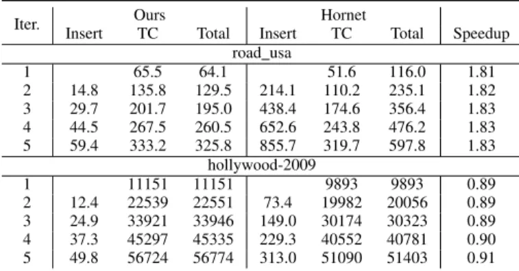
2) Dynamic: For this experiment we pick two datasets, one with a small largest-vertex degree (road usa) and one with a large largest-vertex degree (hollywood-2009). We per-form triangle counting after incrementally inserting edges five times. This scenario was not previously implemented in either Hornet or faimGraph; we implemented it for Hornet only. Table IX shows the result of this experiment. For road usa, our implementation offers a 1.8x speedup over Hornet’s, largely
TABLE VIII: CSR-sort (with CUB) and faimGraph-sort time in ms. Sort time is in general comparable to (and often consid-erably larger than) the time for triangle counting (Table VII).
Dataset Sort CSR Sort faimGraph luxembourg osm 58.13 0.07 germany osm 5260 4.84 road usa 10875 12.65 delaunay n23 3854 18.98 delaunay n20 503.29 2.48 rgg n 2 20 s0 496.85 8.62 rgg n 2 24 s0 7753 178.37 coAuthorsDBLP 136.89 7.36 ldoor 442.15 175.12 soc-LiveJournal1 2226 20428 soc-orkut 1404 41833 hollywood-2009 540.30 8504
TABLE IX: Cumulative time required to perform triangle counting and inserting a batch of size 222 into the graph.
Iter. Ours Hornet
Insert TC Total Insert TC Total Speedup road usa 1 65.5 64.1 51.6 116.0 1.81 2 14.8 135.8 129.5 214.1 110.2 235.1 1.82 3 29.7 201.7 195.0 438.4 174.6 356.4 1.83 4 44.5 267.5 260.5 652.6 243.8 476.2 1.83 5 59.4 333.2 325.8 855.7 319.7 597.8 1.83 hollywood-2009 1 11151 11151 9893 9893 0.89 2 12.4 22539 22551 73.4 19982 20056 0.89 3 24.9 33921 33946 149.0 30174 30323 0.89 4 37.3 45297 45335 229.3 40552 40781 0.90 5 49.8 56724 56774 313.0 51090 51403 0.91
due to our faster insertion. For hollywood-2009, although our insertion performance is around 6x faster than Hornet, Hornet’s faster triangle counting is still fast enough to cover the cost of maintaining sorted adjacency lists. We are 0.9x slower than Hornet on this dataset.
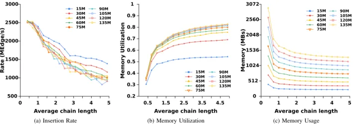
D. Effect of the load factor on our graph data structure To measure the effect of load factor on our hash table, we perform two experiments. Fig. 2 shows our first experiment where we manipulate the chain length of our hash tables by building a graph with the suitable average degree and load factor. As we expect, the insertion throughput of our data structure drops as the chain length increases. On the other hand, the memory utilization increases. This is due to the fact that buckets are now more full. Moreover, the amount of memory used decreases as the average chain length increases. This is due to the fact that fewer buckets are now needed. Fig. 3 shows our second experiment. Similar to the first one, we explore the query performance as the average chain length increases (we use static triangle counting to provide the query workload). The results show the optimal average chain length for our hash table, which is around 0.7.
VII. CONCLUSION ANDFUTUREWORK
Our dynamic GPU graph data structure uses hash tables to represent per-vertex adjacency lists. This representation suits operations that require fast insertion, deletion, and edge lookups, and is superior in performance to previous work that focuses on list data structures for adjacency lists.
In regards to future work, we note that other data structures can be used to represent adjacency lists. For instance, a B-Tree [7] provides a different set of operations as well as main-taining a sorted adjacency list, an optimization that is useful in certain graph algorithms. We also note that supporting hash tables with varying slab sizes may better suit load balancing in scale-free graphs where vertex degrees vary over several orders of magnitude. This would complicate the update procedure at the expense of providing better scalability in graph processing. Moreover, it would require a more complicated dynamic memory allocator design (compared to SlabAlloc used in slab hash [6]) that can support variable-sized memory allocations efficiently.
Although we only discussed phase-concurrent updates and queries in this work, both the slab hash and the B-Tree provide concurrent queries and updates. These concurrent operations can be exposed to a dynamic graph algorithm. The key challenge here is to carefully consider the semantics of these operations. For instance, a graph problem might need to lock a graph node to ensure a consistent view of the adjacency list for the different query and update operations.
ACKNOWLEDGMENTS
This material is based upon work supported by the National Science Foundation under Grant No. CCF-1637442, Grant No. OAC-1740333, and Grant No. CCF-1629657; by DARPA under Grant No. FA8650-18-2-7835; by an Adobe Data Sci-ence Research Award; and by NVIDIA with their funding of an NVIDIA AI Lab at UC Davis. Any opinions, findings, and conclusions or recommendations expressed in this material are those of the authors and do not necessarily reflect the views of the National Science Foundation. This material is based on research sponsored by Air Force Research Lab (AFRL) and the Defense Advanced Research Projects Agency (DARPA) under agreement number FA8650-18-2-7835 and by the U.S. Government under the DARPA SDH program. The views and conclusions contained in this document are those of the authors and should not be interpreted as representing the official policies, either expressed or implied, of the U.S. Government. The U.S. Government is authorized to reproduce and distribute reprints for Governmental purposes notwithstanding any copy-right notation thereon.
Thank you to Mart´ın Farach-Colton, Yuechao Pan, Muham-mad Osama, and Kerry A. Seitz for thoughtful advice and comments on this work.
REFERENCES
[1] F. Busato, O. Green, N. Bombieri, and D. A. Bader, “Hor-net: An efficient data structure for dynamic sparse graphs and matrices on GPUs,” in2018 IEEE High Performance
Rate (MEdge/s)
Average chain length
0 1 2 3 4 5 500 1000 1500 2000 2500 3000 15M 30M 45M 60M 75M 90M 105M 120M 135M
(a) Insertion Rate
Memory Utilization
Average chain length
0.5 1.5 2.5 3.5 4.5 0.2 0.3 0.4 0.5 0.6 0.7 0.8 0.9 1 15M 30M 45M 60M 75M 90M 105M 120M 135M (b) Memory Utilization Memory (MBs)
Average chain length
0 1 2 3 4 5 0 512 1024 1536 2048 2560 3072 15M 30M 45M 60M 75M 90M 105M 120M 135M (c) Memory Usage
Fig. 2: For different directed RMAT graphs with 220 vertices but different average degree (different number of edges), we build the graph using different load factors. (a) The insertion throughput drops by a factor of 2.5 if the hash tables have, on average, chains of length 5. On the other hand, the memory utilization increases (b) and the memory usage decreases (c) as the average chain-length increases.
Time (s)
Average chain length
0 0.5 1 1.5 2 2.5 3 3.5 4 4.5 5 0 50 100 150 200 250 300 15M 30M 45M 60M 75M 90M 105M 120M 135M
Fig. 3: Static triangle counting performance for different undi-rected RMAT graphs with 220 vertices, but different average
degree using hash tables with different load factors. Our data structure achieves its optimal performance when the load factor is around 0.7.
Extreme Computing Conference, ser. HPEC 2018, Sep. 2018.
[2] M. Winter, D. Mlakar, R. Zayer, H.-P. Seidel, and M. Steinberger, “faimGraph: High performance manage-ment of fully-dynamic graphs under tight memory con-straints on the GPU,” in Proceedings of the International Conference for High Performance Computing, Network-ing, Storage, and Analysis, ser. SC ’18, Nov. 2018, pp. 60:1–60:13.
[3] M. Sha, Y. Li, B. He, and K.-L. Tan, “Accelerating
dynamic graph analytics on GPUs,” Proceedings of the VLDB Endowment, vol. 11, no. 1, pp. 107–120, Sep. 2017. [4] Y. Wang, Y. Pan, A. Davidson, Y. Wu, C. Yang, L. Wang, M. Osama, C. Yuan, W. Liu, A. T. Riffel, and J. D. Owens, “Gunrock: GPU graph analytics,” ACM Transactions on Parallel Computing, vol. 4, no. 1, pp. 3:1–3:49, Aug. 2017. [5] M. A. Bender and H. Hu, “An adaptive packed-memory array,” inProceedings of the Twenty-Fifth ACM SIGMOD-SIGACT-SIGART Symposium on Principles of Database Systems, ser. PODS ’06, Jun. 2006, pp. 20–29.
[6] S. Ashkiani, M. Farach-Colton, and J. D. Owens, “A dy-namic hash table for the GPU,” inProceedings of the 31st IEEE International Parallel and Distributed Processing Symposium, ser. IPDPS 2018, May 2018, pp. 419–429. [7] M. A. Awad, S. Ashkiani, R. Johnson, M. Farach-Colton,
and J. D. Owens, “Engineering a high-performance GPU B-tree,” inProceedings of the 24th ACM SIGPLAN Sym-posium on Principles and Practice of Parallel Program-ming, ser. PPoPP 2019, Feb. 2019, pp. 145–157.
[8] D. Merrill, “CUDA UnBound (CUB) library,” 2015, https: //nvlabs.github.io/cub/.