A comprehensive analysis of the correlation between maximal clique size and centrality metrics for complex network graphs

(1)

FULL-LENGTH ARTICLE

A comprehensive analysis of the correlation between

maximal clique size and centrality metrics

for complex network graphs

Natarajan Meghanathan

Computer Science, Jackson State University, Jackson, MS 39217, USA Received 26 December 2015; revised 24 March 2016; accepted 19 June 2016

KEYWORDS

Complex network graphs; Correlation coefficient; Centrality metrics; Maximal clique size

Abstract We seek to identify one or more computationally light-weight centrality metrics that have a high correlation with that of the maximal clique size (the maximum size of the clique a node is part of) - a computationally hard measure. In this pursuit, we compute three well-known mea-sures of evaluating the correlation between two datasets: Product-moment based Pearson’s correla-tion coefficient, Rank-based Spearman’s correlacorrela-tion coefficient and Concordance-based Kendall’s correlation coefficient. We compute the above three correlation coefficient values between the max-imal clique size and each of the four prominent node centrality metrics (degree, eigenvector, betweenness and closeness) for random network graphsand scale-free network graphs as well as for a suite of ten real-world network graphs whose degree distribution ranges from random to scale-free. We also explore the impact of the operating parameters of the theoretical models for gen-erating random networks and scale-free networks on the correlation between maximal clique size and the centrality metrics.

Ó2016 Production and hosting by Elsevier B.V. on behalf of Faculty of Computers and Information, Cairo University. This is an open access article under the CC BY-NC-ND license (http://creativecommons. org/licenses/by-nc-nd/4.0/).

1. Introduction

Network Science (a.k.a. Complex Network Analysis) is an emerging area of interest in the big data paradigm and corre-sponds to analyzing complex real-world networks and

theoret-ical model-based networks from a graph theory point of view. Among the various measures used for complex network anal-ysis, node centrality is a prominently used measure of immense theoretical interest and practical value. The centrality of a node is a link statistics-based quantitative measure of the topo-logical importance of the node with respect to the other nodes in the network [1]. Applications for node centrality metrics could be for example to identify the most influential persons in a social network, the key infrastructure nodes in an Internet, the super-spreaders of a disease, etc. The existing centrality metrics could be broadly classified into two categories [1]: neighbor-based and shortest path-based. Degree centrality (DegC) and Eigenvector centrality (EVC)[2]are well-known E-mail address:[email protected]

Peer review under responsibility of Faculty of Computers and Information, Cairo University.

Production and hosting by Elsevier http://dx.doi.org/10.1016/j.eij.2016.06.004

(2)

measures for neighbor-based centrality, while Betweenness centrality (BWC) [3] and Closeness centrality (ClC) [4] are well-known measures for shortest path-based centrality. Vari-ous time-efficient and space-efficient algorithms (e.g., [5,6]) have been proposed in the literature to determine each of the above centrality metrics. Hence, we refer to node centrality as a computationally light-weight measure.

In addition to node centrality, there exist several other informative measures for quantitatively assessing the impor-tance of a node in a complex network - some of which are too time consuming to determine. We consider one such mea-sure in this paper - the maximal clique size for a node. The maximal clique size for a node is defined as the largest size cli-que the node is part of[7]. A ‘‘clique”in a graph is a subset of the vertices such that there exists an edge between any two ver-tices in the subset[7]. The size of a clique is the number of ver-tices that are part of the clique. Each node in a graph could be part of one or more cliques of different sizes. The largest size clique that a node is part of is of interest for community detec-tion in complex networks (in order to identify nodes that are highly modular). A community of vertices is a subset of the vertices in a graph such that there are more links among ver-tices within this subset and relatively fewer links to verver-tices outside this subset [1]. The effectiveness of the partitioning of a network into communities is evaluated using a metric called the modularity score[8]. The larger the number of ver-tices within a community and larger the number of links between these vertices, the larger the modularity score for the community. Hence, it is of logical interest to identify ver-tices that are highly modular and design algorithms for com-munity detection involving such vertices.

Unfortunately, the problem of determining the maximal cli-que size for a vertex is NP-hard[7]and we refer to it as a com-putationally hard measure. One would have to rely on either time consuming exact algorithms or sub optimal (but relatively less time consuming) approximation heuristics to determine the maximal clique size for a vertex. Also, the focus of the research community has been mostly on developing exact algo-rithms and approximation heuristics (e.g.,[9–11]) for a related problem called the maximum clique size, which is the largest clique size for the entire graph. The maximal clique size for one or more vertices could correspond to the maximum clique size for the graph, but not all vertices are likely to be part of the maximum clique. There could be several vertices in a graph for which the maximal clique size would be less than the max-imum clique size.

Our contributions in this paper are as follows: We seek to identify one or more computationally light-weight centrality metrics that have a high correlation with that of the maximal clique size (a computationally hard measure). In this pursuit, we run the most time-efficient algorithms for each of the four centrality metrics (DegC, EVC, BWC and ClC) and an adapted version of the exact algorithm[9](originally proposed for maximum clique size) to determine the maximal clique size of the vertices in complex networks. We run these algorithms on random networks and scale-free networks generated respec-tively from the well-known Erdos–Renyi[12] and Barabasi– Albert [13] theoretical models as well as on a collection of ten complex real-world networks whose degree distribution ranges from Poisson (random network) to Power-law (scale-free network)[14]. We evaluate the correlation between maxi-mal clique size for a node and each of the four centrality

met-rics using three well-known correlation measures [14]: (i) Pearson’s product-moment based correlation coefficient, (ii) Spearman’s rank based correlation coefficient and (iii) Ken-dall’s concordance based correlation coefficient. We identify the centrality metrics that have the highest correlation as well as the lowest correlation with the maximal clique size with respect to each of the above three correlation measures for ran-dom networks and scale-free networks as well as for each of the ten complex real-world networks. We also identify the cor-relation measures for which we incur the largest and smallest values for the correlation coefficient for different combinations of the centrality metrics, theoretical and real-world networks. In addition, we evaluate the impact of the operating parame-ters of the theoretical models on the nature of the correlation observed between each of the four centrality metrics and max-imal clique size.

The rest of the paper is organized as follows: Section 2

reviews related work on correlation studies involving centrality metrics and maximal/maximum clique size. Section 3 intro-duces the maximal clique size of a graph and describes an exact algorithm to determine the same. Section 4 reviews the two neighbor-based centrality metrics (DegC and EVC) and the two shortest path-based centrality metrics (BWC and ClC) and briefly describes an efficient algorithm to determine each of them. Section5introduces the three measures for evaluating the correlation coefficient between node centrality and maxi-mal clique size per node. Section 6 presents the ten real-world network graphs and discusses the results for correlation coefficient analysis. Sections 7 and 8respectively present the results for correlation coefficient analysis on random network graphs (generated from the Erdos–Renyi model) and scale-free network graphs (generated from the Barabasi–Albert model). Section 9 concludes the paper. Throughout the paper, the terms ’node’ and ’vertex’ as well as ’link’ and ’edge’ are used interchangeably. Likewise, a vertex might be referred to as either i or vi. They mean the same. We model all the theoretical-model generated graphs and the real-world net-work graphs as undirected graphs.

2. Related work

Recently, we published two articles[23,24]analyzing the corre-lation between the maximal clique size and the centrality met-rics for complex real-world network graphs. The two articles are restricted to just using the Pearson’s product moment-based correlation measure and analyzed only six of the ten real-world networks studied in this paper. In this paper, in addition to the Pearson’s measure, we have also used two other correlation measures (Spearman’s rank-based and Kendall’s concordance-based measures) so that we are able to identify the best-case and worst-case levels of correlation between max-imal clique size and the centrality metrics. We have also expanded the pool of complex networks analyzed to include the theoretical networks generated from the Erdos–Renyi (ER) model (for random networks) and the Barabasi–Albert (BA) model (for scale-free networks) as well as included four more real-world networks (thus covering a comprehensive set of ten real-world networks with degree distribution ranging from random to scale-free). We observe that it is possible to directly associate the correlation levels with the state of the ran-dom networks in the supercritical and fully connected regimes

(3)

using the Pearson’s product moment-based correlation mea-sure. In addition, centrality metrics have also been widely stud-ied for the analysis and visualization of complex networks in several domains, ranging from biological networks to social networks [27,28]. With regard to the maximal clique size of the individual vertices (the largest size clique that a vertex is part of), in[29]: the distribution of the maximal clique size val-ues for the vertices in several real-world network graphs as well as those of the small-world networks (under the evolution of the Watts–Strogatz model [30]) has been observed to follow a Poisson-style distribution. Most of the other works in the lit-erature focused on developing efficient approximation heuris-tics as well as exact algorithms to determine the maximum clique size (an NP-hard problem) for the entire network graphs. Though branch-and-bound has been the common theme among the exact algorithms to determine the maximum clique size, the difference lies in the approach used to prune the search space: node degree[9], vertex coloring[10]and vertex ordering[11]. As is observed in this paper, the savings in time (due to pruning) incurred by the branch-and-bound based exact algorithms for maximum clique size of an entire graph is lost to a certain extent when these algorithms are adapted to determine the maximal clique size of the individual vertices of the graph. Owing to the time-consuming nature of the exact algorithms to determine maximal clique size of the vertices in a graph, it becomes imperative to identify one or more computa-tionally light-weight metrics (like the degree centrality) that can be used to rank the vertices in a complex network graph in almost the same order (if not exact) that would be obtained using the maximal clique size.

3. Maximal clique size

The maximal clique size of a node is the largest size clique that the node is part of. The maximal clique size of a node is a measure of the level of modularity of the node and could be used

recently proposed exact algorithm by Pattabiraman et al.[9]

for maximum clique size of a graph and slightly modify it to determine the maximal clique size of the individual vertices in a graph.

3.1. Original exact algorithm to determine maximum clique size for a graph

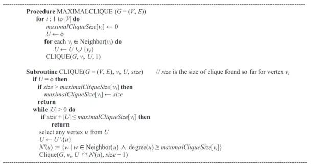
The original exact algorithm by Pattabiraman et al.[9]follows a branch and bound approach of searching through all possi-ble cliques and limiting the exploration only to vertices whose agglomeration has scope of being larger than the size of the largest clique known until then.Fig. 1illustrates the pseudo code of the exact algorithm for maximum clique size. As one can notice, the algorithm uses a variablemax to keep track of the largest size clique determined during the search process. The procedure MAXCLIQUE proceeds in iterations, and in theith iteration, the algorithm explores whether a clique of size greater than the current value of max could be determined involving vertexvi(the vertices are considered in the increasing order of their IDs) and its neighbors. For each such vertexvi, a candidate set of verticesUis constructed involvingvi’s neigh-bors (each of whose degree is at least the value ofmax) and is passed to the subroutine CLIQUE along with a variablesize whose value at any time during the execution of the subroutine represents the size of the largest clique known until then involving vertexviand its neighbors.

The subroutine CLIQUE expands the size of the clique involvingviwith one vertex at a time (starting withviitself) through a combination of iterations and recursions. In each such iteration, a random node uis removed from the set U passed to the subroutine and the setUis filtered to retain only those vertices that are also neighbors of the nodeu; the value ofsizeis incremented by 1 to account for the inclusion of node uto the clique and a recursive call to CLIQUE is made with the updatedUand value ofsize. A recursive call to the

(4)

tine CLIQUE runs as long as the current value ofmaxis less than the sum of the size of the setUpassed to the subroutine and thesizeof the current clique found until then. During the sequence of returns from the recursive calls, it is also possible that a different neighbor nodeuofvigets selected and the size of the clique involving the new nodeuand its neighbors along withvicould be larger the current value ofmax. Also, during any such recursive call to CLIQUE, if the size of the setU reaches zero, the algorithm terminates the sequence of recur-sions and updates the value ofmaxif it is less than thesize of the clique found until then involving vertex vi and its neighbors.

The efficiency of the algorithm is severely impacted by the order the vertices are considered for the iterations. A labeling of the vertices in the decreasing order of their degree increases the chances of finding the maximum size clique much earlier than a random labeling of the vertices[9]. If the maximum size clique is found in the earlier iterations itself, the subsequent iterations could end up to be mere pruning operations if the vertices involved in these iterations have a degree smaller than the maximum size clique determined until then.

3.2. Modified exact algorithm to determine maximal clique size for a vertex

Fig. 2illustrates the pseudo code that we propose for a

mod-ified exact algorithm to determine the maximal clique size for any vertex in a given graph. Unlike the procedure MAXI-MUMCLIQUE (discussed in Section3.1), we can no longer discard vertices with degree lower than the maximum clique size found until then for the entire graph. We need to run the procedure for every vertex to determine the maximal clique size involving the vertex.

For each vertexvi, to start with, the maximal clique size known until then is 0; so, we construct the candidate set of ver-tices (U) involving all the neighbors ofviand pass them to the subroutine CLIQUE. We could retain all the pruning strate-gies (discussed in Section3.1) in the subroutine CLIQUE: we need not explore nodeu(chosen from the setU) and its

neigh-bors if their degree is smaller than the value ofsize(the max-imal clique size involving vertex vi) known until then. For speedup, we list the neighbors of a vertexviin the initial set U passed from the procedure MAXIMAL CLIQUE to the subroutine CLIQUE in the decreasing order of their degree.

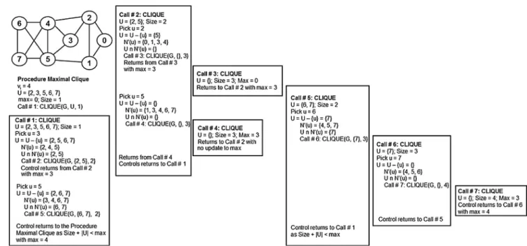
Fig. 3presents an example to illustrate the execution of the modified exact algorithm to determine the maximal clique size for a vertex. We consider vertexvi= 4 as the vertex for which we want to find the maximal clique size. We identify each recursive call to the subroutine CLIQUE with a unique identi-fication number (Call # 1, 2, etc.) so that it is easy trace the exe-cution of the algorithm. The first few recursive calls (Call #s 1– 2–3–4) lead to the identification of clique {4, 2, 3} of size 3. However, the next set of recursive calls (Call #s: 1–5–6–7) leads to the identification of the maximal size clique {4, 5, 6, 7} involving vertex 4. Fig. 4illustrates the maximal clique size of all the vertices in the sample graph used inFig. 3.

4. Node centrality metrics

We now review the centrality metrics that are used for the cor-relation coefficient analysis studied in this paper. These are the neighbor-based degree centrality (DegC) and eigenvector cen-trality (EVC) metrics and the shortest path-based betweenness centrality (BWC) and closeness centrality (ClC) metrics. 4.1. Degree centrality

The degree centrality of a vertex is the number of neighbors for the vertex in the graph and can be easily computed by counting the number of edges incident on the vertex. If A is thenn adjacency matrix for a graph such thatA[i,j] = 1 if there is an edge connecting vi to vj(for undirected graphs) and A[i, j] = 0 if there is no edge connectingviandvj.

The degree centrality of a vertexviis quantitatively defined as follows: DegC(vi) =

Pn

j¼1A½i;j.Fig. 5illustrates an

exam-ple for computing the degree centrality of all the vertices in a graph as the product of the adjacency matrix of the graph

(5)

and a unit column vector of 1 s corresponding to the number of vertices in the graph.

4.2. Eigenvector centrality

The eigenvector centrality (EVC) of a vertex is a quantitative measure of the degree of the vertex as well as the degree of its neighbors. A vertex that has a high degree for itself as well as located in the neighborhood of high-degree vertices is likely to have a larger EVC. The EVC values of the vertices in a graph correspond to the entries for the vertices in the principal

eigenvector of the adjacency matrix of the graph. An nn adjacency matrix has n eigenvalues and the corresponding eigenvectors. The principal eigenvector is the eigenvector cor-responding to the largest eigenvalue (principal eigenvalue) of the adjacency matrix,A. Moreover, if all the entries in a square matrix are positive (i.e., greater than or equal to zero), the principal eigenvalue as well as the entries in the principal eigen-vector is also positive[15].

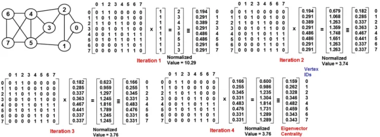
We determine the EVC of the vertices using the Power-iteration method[15]. According to this method, we start with a unit vectorX0= [1 1 1 1. . .1 1] of all 1 s corresponding to

the number of vertices in the graph and go through a sequence of iterations. The tentative eigenvector computed during the (i+ 1)th iteration is given as follows: AXi/||AXi||, where ||AXi|| is the normalized value of the vector resulting from the product of the adjacency matrix and the tentative eigenvec-tor computed during theith iteration. We continue the itera-tions until the normalized value ||AXi|| does not change significantly and converges to a constant value (when rounded to the second decimal). The normalized value at this juncture also corresponds to the principal eigenvalue of the adjacency matrix and the tentative eigenvector computed with this normalized value corresponds to the principal eigenvector of Figure 3 Example to illustrate the execution of the exact algorithm to determine maximal clique size of a vertex.

Figure 4 Maximal clique size of the vertices in a sample graph.

(6)

the adjacency matrix. We illustrate the execution of the Power-iteration method with the example shown inFig. 6. As can be noticed inFig. 6, even though both vertices 4 and 5 have the same larger degree (five) - the EVC of vertex 4 is larger than the EVC of vertex 5 - this could be attributed to the degree dis-tribution {3, 3, 3, 4, 5} of the neighbors of vertex 4 vis-a-vis the degree distribution {3, 3, 3, 2, 5} of the neighbors of vertex 5. 4.3. Betweenness centrality

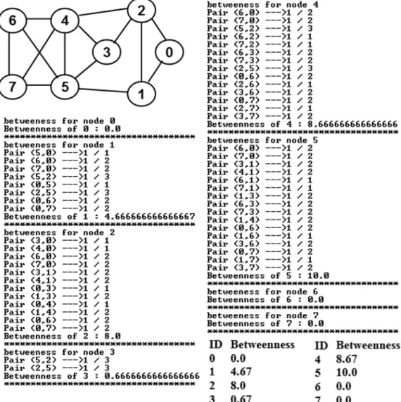
The betweenness centrality (BWC) of a vertex is the sum of the fraction of shortest paths going through the vertex between any two vertices, considered over all pairs of vertices. In this paper, we determine the BWC of the vertices using the Breadth First Search (BFS)-variant of the well-known Brandes’ algo-rithm[5]. We run the BFS algorithm on each vertex in the graph and determine the level of each vertex (the number of hops/edges from the root) in each of these BFS trees. The root of a BFS tree is said to be at level 0 and the number of shortest paths from the root to itself is 1. On a BFS tree rooted at ver-tex r, the number of shortest paths for a vertex i at level l (l> 0) from the rootr is the sum of the number of shortest paths from the root r to each the neighbors of vertex i (in the original graph) that are at levell1 in the BFS tree.

Since we are working on undirected graphs, the total num-ber of shortest paths from vertexito vertexj(denotedspij) is simply the number of shortest paths from vertexito vertexjin the shortest path tree rooted at vertexior vice versa. The num-ber of shortest paths from a vertex i to a vertex j that go through a vertex k (denoted spij(k)) is the maximum of the number of shortest paths from vertexito vertexkin the short-est path tree rooted atiand the number of shortest paths from vertexjto vertexkin the shortest path tree rooted at vertexj. Thus, BWC(k) =Pk–i

k–j spijðkÞ

spij .

Fig. 7illustrates an example to calculate the BWC of

ver-tices in the same graph used in Figs. 3–6. We can observe the betweenness values for vertices 0, 6 and 7 are zero each, because no shortest path between any two vertices goes through them. We observe that even though vertices 4 and 5 have the same larger degree, the average degree of the

neigh-bors of vertex 5 is slightly lower than the average degree of the neighbors of vertex. As a result, vertex 5 is more likely to occupy a relatively larger fraction of the shortest path between any two vertices and incur a relatively larger BWC value compared to vertex 4 (even though vertex 4 has a larger EVC value). Also, even though vertex 3 has a larger degree than vertex 1, the BWC of vertex 1 is significantly larger than that of vertex 3. This could be attributed to vertex 1 lying on the shortest path from vertices 0 and 2 to vertices 4, 5, 6 and 7; on the other hand, vertex 3 lies only on the shortest path between 2 and 5.

4.4. Closeness centrality

The closeness centrality (ClC) of a vertex is the inverse of the sum of the number of shortest paths from the vertex to every other vertex in the graph. We determine the ClC of the vertices by running the BFS algorithm on each vertex and summing the number of shortest paths from the root vertex to every other vertex in these BFS trees. Fig. 8 illustrates an example to compute the ClC of the vertices. We observe vertices with a larger degree are more likely to have shortest paths of lower hop count to the rest of the vertices, leading to a larger ClC value.

5. Correlation coefficient measures

We now discuss the three well-known correlation coefficient measures that are used to evaluate the correlation between maximal clique size and the four centrality metrics presented in Section 4. These are the Product-moment based Pearson’s correlation coefficient, Rank based Spearman’s correlation coefficient and Concordance based Kendall’s correlation coef-ficient. All the three measures evaluate the extent of the degree of linear dependence between two datasets or performance metrics (in our case, the maximal clique size and each of the four centrality metrics)[14].

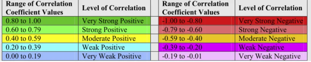
The correlation coefficient values obtained for all the three measures range from -1 to 1. Correlation coefficient values clo-ser to 1 indicate a stronger positive correlation between the Figure 6 Example to illustrate the calculation of eigenvector centrality using power iteration method.

(7)

two metrics considered (i.e., a vertex having a larger value for one of the two metrics is more likely to have a larger value for the other metric too), while values closer to -1 indicate a stron-ger negative correlation (i.e., a vertex having a larstron-ger value for one of the two metrics is more likely to have a smaller value for the other metric). Correlation coefficient values closer to 0 indicate no correlation (i.e., the values incurred by a vertex

for the two metrics are independent of each other). We will adopt the ranges (rounded to two decimals) proposed by Evans[16]to indicate the various levels of correlation, shown inTable 1. The color code to be used for the various levels of correlation is also shown in this table.

For simplicity, we refer to the two datasets asM and C respectively corresponding to the maximal clique size and Figure 7 Example to illustrate the calculation of betweenness centrality.

(8)

centrality. We will use the results fromFigs. 4–8to illustrate examples for the computation of the correlation coefficient under each of the three measures.

5.1. Pearson’s product moment-based correlation coefficient The Pearson’s product moment-based correlation coefficient for two datasets is defined as the covariance of the two datasets divided by the product of their standard deviation [14]. Let MavgandCavgdenote the average values for the maximal cli-que size and a centrality metric for a graph ofnvertices and letMiandCidenote respectively the values for the maximal clique size and the centrality metric of interest incurred for ver-texi. The Pearson’s correlation coefficient (indicated PCC) is quantitatively defined as shown in Eq.(1). The term product moment is associated with the product of the mean (first moment) adjusted values for the two metrics in the numerator of the formulation.Fig. 9presents the calculation of the PCC for the maximal clique size (M) and degree centrality (C) val-ues obtained for the example graph used in Figs. 3–8. We obtain a Correlation Coefficient value of 0.5 (seeFig. 9) indi-cating a moderately positive correlation between the two met-rics for the example graph.

PCCðM;CÞ ¼ Pn i¼1ðMiMavgÞðCiCavgÞ ffiffiffiffiffiffiffiffiffiffiffiffiffiffiffiffiffiffiffiffiffiffiffiffiffiffiffiffiffiffiffiffiffiffiffiffiffiffiffiffiffiffiffiffiffiffiffiffiffiffiffiffiffiffiffiffiffiffiffiffiffiffiffiffiffiffiffiffiffiffiffiffi Pn i¼1ðMiMavgÞ 2Pn i¼1ðCiCavgÞ 2 q : ð1Þ

5.2. Spearman’s rank-based correlation coefficient

Spearman’s rank correlation coefficient (SCC) is a measure of how well the relationship between two datasets (variables) can be assessed using a monotonic function[14]. To compute the

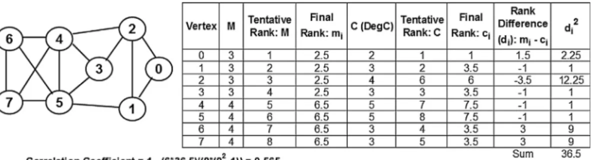
SCC of two datasetsMandC, we convert the raw scoresMi andCifor a vertexito ranksmiandciand use formula(2) shown below, where di=mici is the difference between the ranks of vertexiin the two datasets. We follow the conven-tion of assigning the rank values from 1 tonfor a graph ofn vertices, even though the vertex IDs range from 0 ton1. To obtain the rank for a vertex based on the list of values for a performance metric, we first sort the values (in ascending order). If there is any tie, we break the tie in favor of the vertex with a lower ID; we will thus be able to arrive at a tentative, but unique, rank value for each vertex with respect to the per-formance metric. We determine a final ranking of the vertices as follows: For vertices with unique value of the performance metric, the final ranking is the same as the tentative ranking. For vertices with an identical value for the performance metric, the final ranking is assigned to be the average of their tentative rankings. Fig. 10illustrates the computation of the tentative and final ranking of the vertices based on their maximal clique size and degree centrality values in the example graph used in

Figs. 3–9 as well as illustrates the computation of the

Spear-man’s rank-based correlation coefficient. SCCðM;CÞ ¼1 6 Pn i¼1d 2 i nðn2₁_Þ: ð2Þ

InFig. 10, we observe ties among vertices with respect to

both the maximal clique size and degree centrality. The tenta-tive ranking is obtained by breaking the ties in favor of vertices with lower IDs. In the case of maximal clique size (M), we observe the four vertices 0–3 having an identical Mvalue of 3 each and their tentative rankings are 1–4; the final ranking (2.5) of each of these four vertices is thus the average of 1, 2, 3 and 4. Likewise, the four vertices 4–7 have an identical M value of 4 each and their tentative rankings are 5–8; the final Table 1 Range of correlation coefficient values and the corresponding levels of correlation.

Figure 9 Example to illustrate the computation of Pearson’s correlation coefficient (between maximal clique size: Mand degree centrality:C).

(9)

ranking (6.5) of each of these four vertices is thus the average of 5, 6, 7 and 8. In the case of degree centrality (D), we observe ties among vertices with degree 3 (tentative rankings of 2, 4 and 5; final ranking: 3.5 - average of 2, 4 and 5) and among vertices with degree 5 (tentative rankings of 7 and 8; final rank-ing: 7.5 - average of 7 and 8). The Spearman’s rank-based cor-relation coefficient (SCC) computed for maximal clique size and degree centrality for the example graph used fromFigs. 3– 9is 0.565. We observe the SCC value to be slightly larger than the PCC value obtained inFig. 9for the same graph, but, the level of correlation for both the measures still falls in the range of moderately positive correlation.

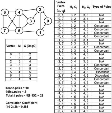
5.3. Kendall’s Concordance-based Correlation Coefficient Kendall’s concordance-based correlation coefficient (KCC) for any two performance metrics (say,MandC) is a measure of the similarity (a.k.a. concordance) in the ordering of the values for the metrics incurred by the vertices in the graph[14]. We define a pair of distinct vertices vi and vj as concordant if {Mi>MjandCi> Cj} or {Mi<MjandCi<Cj}. In other words, a pair of vertices vi and vj are concordant if either one of these two vertices strictly has a larger value for the two metricsMandCcompared to the other vertex. We define a pair of distinct verticesviandvjas discordant if {Mi>Mj andCi<Cj} or {Mi<MjandCi>Cj}. In other words, a pair of verticesviandvjare discordant if a vertex has a larger value for only one of the two performance metrics. A pair of distinct verticesviandvjare neither concordant nor discordant if either {Mi=Mj} or {Ci=Cj} or {Mi=MjandCi=Cj}. The Kendall’s concordance-based correlation coefficient is simply the difference between the number of concordant pairs (denoted #conc.pairs) and the number of discordant pairs (#disc.pairs) divided by the total number of pairs considered. For a graph of n vertices, KCC is calculated as shown in formulation(3).

KCCðM;CÞ ¼#conc:pairs₁ #disc:pairs

2nðn1Þ

: ð3Þ

Fig. 11illustrates the calculation of the Kendall’s correla-tion coefficient between maximal clique size and degree cen-trality for the example graph used inFigs. 3–9. For a graph of 8 vertices, the total number of distinct pairs that could be considered is 8(8–1)/2 = 28 and out of these, 10 pairs are classified to be concordant and 2 pairs as discordant. The

remaining 16 pairs are neither concordant nor discordant (denoted as N/A) in the figure. We get a correlation coefficient of 0.286, falling in the range of weakly positive correlation, and it is lower than the correlation coefficient values (falling in the range of moderately positive correlation) obtained with the Pearson’s and Spearman’s measures. The KCC is also observed to return the lowest correlation coefficient values for all our experiments with theoretical and real-world com-plex networks (Sections8). Thus, the KCC could be construed to provide a lower bound for the correlation coefficient values and the level of correlation between maximal clique size and the centrality metric considered.

6. Real-world network graphs

We consider a suite of ten real-world network graphs for our correlation analysis. We list below and identify these graphs in the increasing order of their variation in node degree, cap-tured in the form of a metric called the spectral radius ratio for node degree (denotedksp) [17]. The spectral radius ratio for node degree for a graph is the ratio of the principal eigen-value of the adjacency matrix of the graph to that of the aver-age node degree. The ksp values are always greater than or equal to 1.0. The larger the value, the larger the variation in node degree. Thekspvalues of the real-world networks consid-ered in this paper range from 1.01 to 3.22 (i.e., from random networks to scale-free networks). Random networks exhibit a Poisson-style degree distribution and have a lower variation in node degree; their ksp values are typically closer to 1.0. Scale-free networks have a larger variation in node degree (especially those like the US Airport Networks that have a few hubs - high degree nodes, and the rest of the nodes are of relatively much lower degree) - incurring a largerkspvalue. The real-world network graphs [18–20] are briefly intro-duced below, in the increasing order of theirkspvalue. We also identify these networks with their ID (ranging from 1 to 10 as listed below) as well as with a twocharacter abbreviation -listed along with thekspvalue.

(1) US Football Network (FN; ksp= 1.01): This is a network of 115 football teams (nodes) of US universities that played in the Fall 2000 season; there is an edge between two nodes if the corresponding teams have played at least once against each other in the past.

Figure 10 Example to illustrate the computation of Spearman’s correlation coefficient (between maximal clique size:Mand degree centrality:C).

(10)

(2) Dolphin Network (DN;ksp= 1.40): This is a network of 62 dolphins (nodes) that lived in the Doubtful Sound fiord of New Zealand; there is an edge between two nodes if the corresponding dolphins were seen moving with each other during the observation period.

(3) US Politics Book Network (PN;ksp= 1.42): This is a network of 105 books (nodes) related to US Politics that were sold in Amazon.com; there is an edge between two nodes if customers who bought one of the two books also bought the other book and vice versa.

(4) Karate Network (KN;ksp= 1.47): This is a network of 34 members (nodes) of a Karate Club at a US university in the 1970 s; there is an edge between two nodes if the corresponding members were seen interacting with each other during the observation period.

(5) C. Elegans Neural Network (NN;ksp= 1.68): This is a network of 297 neurons (nodes) in the neural network of the hermaphrodite Caenorhabditis Elegans; there is an edge between two nodes if the corresponding neurons interact with each other (in the form of chemical synapses, gap junctions and neuromuscular junctions). (6) Word Adjacency Network (WN;ksp= 1.73): This is a

network of 112 adjectives and nouns (nodes) in the novel David Copperfield by Charles Dickens; there exists an edge between two nodes if the corresponding words occurred adjacent to each other at least once in the novel.

(7) Les Miserables Network (LN;ksp= 1.82): This is a net-work of 77 characters (nodes) in the novel Les Miser-ables; there exists an edge between two nodes if the corresponding characters appeared together in at least one of the chapters in the novel.

(8) Citation Graph Drawing Network (CN; ksp= 2.24): This is a network of 311 papers (nodes) that were pub-lished in the Proceedings of the Graph Drawing (GD) conferences from 1994 to 2000 and cited in the papers published in the GD’2001 conference. There is an edge between two nodes if one of the papers has cited the other paper as a reference. Even though this network is to be modeled as a directed graph, for simplicity and consistency with the rest of the networks consid-ered, we model this network as an undirected graph. (9) Erdos Collaboration Network (EN;ksp= 2.28): This is

a network of 472 authors (nodes) who have either directly published an article with Paul Erdos or through a chain of collaborators leading to Paul Erdos. There is an edge between two nodes if the corresponding authors have co-authored at least one publication.

(10) US Airports Network (AN:ksp= 3.22): This is a net-work of 332 airports (nodes) in the US in the year 1997. There is an edge between two nodes if there is a direct flight connection between the corresponding airports.

Figure 11 Example to illustrate the computation of Kendall’s correlation coefficient (between maximal clique size:M and degree centrality:C).

(11)

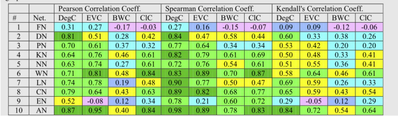
Table 2 presents the raw values for the correlation coeffi-cient obtained for the maximal clique size and each of the four centrality metrics based on the PCC, SCC and KCC measures. We color code the levels of correlation in these tables accord-ing to the color codes listed inTable 1. The overall trend of the results displayed inTable 2is that the neighbor-based central-ity metrics (degree centralcentral-ity and eigenvector centralcentral-ity) exhibit relatively stronger positive correlation compared to the short-est path-based centrality metrics (betweenness and closeness centrality). The correlation coefficient values were observed to be positive for at least nine of the ten real-world networks for each centrality metric under each of the three correlation measures. With respect to the trend of correlation with increas-ing values for the spectral radius ratio for node degree, we observe the overall trend to be an increase in the strength of correlation between the maximal clique size and the centrality metrics with increase in the variation in node degree. Thus, as the real-world networks are relatively more scale-free (which is the case in reality), we could expect to see a much better strong correlation between maximal clique size and the centrality met-rics, at least for the neighbor-based centrality metrics.

The degree centrality exhibits a strong-very strong positive correlation with the maximal clique size for eight of the ten real-world networks under the Pearson’s measure and for nine of the ten networks under the Spearman’s measure. Even with the Kendall’s scheme, we observe the degree centrality to exhi-bit a moderately positive correlation for four of the ten net-works and strong-very strong positive correlation for another four of the ten networks. The eigenvector centrality exhibits a strong-very strong positive correlation for seven of the ten real-world networks under both the Pearson’s and Spearman’s correlation coefficient measures and exhibits a moderately pos-itive correlation for five of the ten networks under the Ken-dall’s correlation measure.

The best-case performance for the shortest path-based cen-trality metrics is a strong-very strong positive correlation for five-six of the ten real-world networks under the Spearman’s correlation coefficient measure. The shortest path-based cen-trality metrics exhibit very weak negative-weak positive corre-lation with the maximal clique size for five-seven of the ten real-world under the Kendall’s correlation measure. Overall, we could say the betweenness centrality exhibits the weakest correlation to that of the maximal clique size. Under the Pearson’s correlation measure, we observe the betweenness

centrality to exhibit weak-very weak positive correlation for five of the ten networks, moderately positive correlation with four of the ten networks and very weak negative correlation for the random network-type US Football network. Rela-tively, the closeness centrality appears to exhibit a better corre-lation with the maximal clique size. The closeness centrality metric exhibits a strong-very strong correlation for at least five of the ten real-world networks under the Pearson’s and Spear-man’s correlation measures.

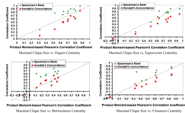
FromFig. 12, we observe the Pearson’s and Spearman’s

correlation coefficient measures to yield higher correlation coefficient values between maximal clique size and the three centrality metrics, except the betweenness centrality. Likewise, we observe the Kendall’s correlation coefficient measure to serve as a lower bound for the correlation between the maxi-mal clique size and the three centrality metrics, except the betweenness centrality. For the betweenness centrality, we observe Pearson’s correlation coefficient to be relatively the lowest for a majority of the real-world networks, whereas the Spearman’s correlation coefficient appeared to be relatively the largest. With regard to the proximity of the correlation coefficient values under the three measures (this could be deter-mined by examining whether or not the data points lie close to or on the diagonal line in the plots shown in Fig. 12), we observe the Pearson’s and Spearman’s correlation coefficient values to be relatively closer to each other when used to eval-uate the correlation between maximal clique size vs. eigenvec-tor centrality as well as for maximal clique size vs. closeness centrality. On the other hand, we observe the Pearson’s and Kendall’s correlation coefficient values to be relatively closer to each other when used to evaluate the correlation between maximal clique size and betweenness centrality.

Based on the above discussion and from the distribution of the data points inFig. 13, we could confidently conclude that the degree centrality metric exhibits the strongest correlation with the maximal clique size under all the three correlation measures for a majority of the real-world networks analyzed in this paper. InFig. 13, we observe a majority of the data points corresponding to eigenvector centrality and closeness centrality to lie below the diagonal line when plotted against the degree centrality for each of the three correlation measures. Since the betweenness centrality incurred the smallest values for the correlation coefficient in all the cases, we did not use the BWC metric in these plots.

(12)

7. Random network graphs

In this section, we discuss the results of our correlation analy-sis studies for maximal clique size vs. centrality metrics on the random network graphs generated from the well-known Erdos–Renyi (ER) model [12]. Under the ER model, there could exist a link between any two nodes in the network with a probabilityplink. We conduct the simulations for a network of 100 nodes and vary theplinkvalues from 0.01 to 0.50. For eachplinkvalue, we run 100 runs of the simulations and aver-age the results for the correlation coefficient with maximal cli-que size for each centrality metric under each of the three correlation measures. For a givenplinkvalue, we consider all pairs of nodes in the network and set up a link between any two nodes if the random number (in the range 0. . .1) generated for the pair of nodes is less than or equal toplink.

The larger the plink value, the larger the number of links generated in a random network and lower the variation in node degree (measured in terms of the spectral radius ratio for node degree). With a larger number of links for a fixed number of nodes, the robustness of the network (with regard

to disconnection due to link failures) also increases (as is mea-sured in terms of the algebraic connectivity of the network). The algebraic connectivity [21]of a connected network is the second smallest eigenvalue of the Laplacian matrix[14] of a graph. If AandD are respectively the adjacency matrix and degree matrix of a graph, the Laplacian matrix L is simply A–D. The degree matrix is also a square matrix whose non-diagonal entries are all zeros and the non-diagonal entries corre-spond to the degree of the vertices. FromFig. 14, we observe Maximal Clique Size vs. Degree Centrality Maximal Clique Size vs. Eigenvector Centrality

Maximal Clique Size vs. Betweenness Centrality Maximal Clique Size vs. Closeness Centrality

Figure 12 Distribution of the correlation coefficient values for real-world networks (from the correlation measures viewpoint).

Pearson's Correlation Measure Spearman's Correlation Measure Kendall's Correlation Measure Figure 13 Distribution of the correlation coefficient values for real-world networks (from the centrality metrics viewpoint).

Figure 14 Spectral radius and algebraic connectivity of random networks under the ER model.

(13)

the spectral radius ratio for node degree to show a sharp decrease (a power-law style decrease) with increase in plink, whereas the algebraic connectivity exhibits a moderate rate of increase with increase inplink.

With respect to the correlation measures used, fromFig. 15, we observe the Spearman’s rank-based correlation and Ken-dall’s concordance-based correlation measures to respectively serve as an upper bound and lower bound for the level of cor-relation. All the four centrality metrics incur relatively closer values for the correlation coefficient under the Pearson’s and Spearman’s correlation measures to an extent that the level of correlation between a centrality metric and maximal clique size is the same under both the measures for a majority of the plinkvalues. As in the case of real-world networks, the between-ness centrality incurs the lowest correlation coefficient values with maximal clique size under all the three correlation measures. Hence, when we just plot the correlation coefficient values of the three centrality metrics under a particular corre-lation measure (Fig. 16), forplinkvalues greater than or equal to 0.05 (referred to as the fully connected regime: see the dis-cussion below), we observe a negligible difference in the level of correlation for DegC, EVC and ClC with maximal clique size, with the EVC incurring slightly larger correlation coeffi-cient values (the maximum difference is within 0.05 for plinkP0.1).

FromFig. 15, we observe that for random networks with

plink values starting from 0.05, the level of correlation (for any centrality metric with the maximal clique size under any of the three correlation measures) is at best moderately

posi-tive. The degree centrality and closeness centrality metrics exhibit strong-very strong positive correlation (a decrease in the level of correlation asplinkincreases) forplinkvalues rang-ing from 0.01 to 0.04 (scenarios when the variation in node degree is larger, and the connectivity of the network is low). The eigenvector centrality metric exhibits weak-moderate pos-itive correlation (an increase in the level of correlation asplink increases) for plink values ranging from 0.01 to 0.04 and the level of correlation remains the same for plink values greater than or equal to 0.05. The betweenness centrality metric exhi-bits a relatively higher level of correlation forplinkvalues 0.01 to 0.09, compared to the level of correlation observed forplink values greater than or equal to 0.1. Thus, for at least three of the four centrality metrics, the transition from a relatively higher or lower level of positive correlation to at best a mod-erately positive level of correlation (that remains the same henceforth) occurs at plink value of 0.05 (for a network of n= 100 nodes,plink= 0.05ln(n)/n) and this could be ter-med as the critical probability at which the random network is considered to be in the fully connected regime[22]and has a single giant component with no isolated nodes or clusters. For plinkP1/n (i.e., plinkP0.01 for n= 100 nodes) and plink< ln(n)/n, we could refer to the random network to be in the supercritical regime[22]with a single giant component, but with one or more isolated nodes or clusters. Hence, for a random network under evolution according to the ER model, we could conclude that the centrality metrics exhibit at best a moderately positive correlation with the maximal clique size in the fully connected regime, whereas the degree centrality and Maximal Clique Size vs. Betweenness Centrality Maximal Clique Size vs. Closeness Centrality

Figure 15 Distribution of the correlation coefficient values for the ER model based-random networks (from the correlation measures viewpoint).

Pearson's Correlation Measure Spearman's Correlation Measure Kendall's Correlation Measure Figure 16 Distribution of the correlation coefficient values for the ER model based-random networks (from the centrality metrics viewpoint).

(14)

closeness centrality metrics exhibit a strong-very strong posi-tive correlation with the maximal clique size in the supercritical regime.

8. Scale-free network graphs

In this section, we discuss the results of correlation analysis obtained for scale-free network graphs generated from the well-known Barabasi Albert (BA) model[13]. The BA model

for network evolution is based on the notion of preferential attachment: i.e., a newly introduced node prefers to attach itself to nodes with relatively larger degree. In addition to the total number of nodes (n) in the network, the BA model works based on two parameters: the initial number of nodes (n0) and the initial number of links added per node

introduc-tion (m0). We start with a network ofn0nodes (identified with

ids 1,. . .,n0) such that there exists at least one link incident on

each node. We then start introducing new nodes to the net-work, one node at a time, and these nodes are identified based

Figure 17 Spectral radius and algebraic connectivity of scale-free networks under the BA model.

Initial Number of Nodes,n0= 3 Initial Number of Nodes,n0= 10 Initial Number of Nodes,n0 = 20

Maximal Clique vs. Degree Centrality

Initial Number of Nodes,n0= 3 Initial Number of Nodes,n0= 10 Initial Number of Nodes,n0= 20

Maximal Clique vs. Eigenvector Centrality

Initial Number of Nodes,n0= 3 Initial Number of Nodes,n0= 10 Initial Number of Nodes,n0 = 20

Maximal Clique vs. Betweenness Centrality

Initial Number of Nodes,n0= 3 Initial Number of Nodes,n0= 10 Initial Number of Nodes,n0= 20

Maximal Clique vs. Closeness Centrality

Figure 18 Distribution of the correlation coefficient values for the BA model based scale-free networks (from the correlation measures viewpoint).

(15)

i.e.A[j,t+ 1] = 0 forj= 1,. . .,t, whereAis the adjacency matrix of the network graph) are considered while computing the above probability formulation for adding each of them0

links to the newly introduced node.

For the simulations, we generated scale-free networks com-prising of n= 100 nodes and varied the initial number of nodes and links respectively with values of n0= 3, 10 and

20, andm0= 2, 3,. . ., 20 (in increments of 1). For a fixedn0

andm0, we ran the simulations 100 times and averaged the

results for the correlation coefficient values obtained for max-imal clique size with each of the four centrality metrics under each of the three correlation measures. Fig. 17 displays the impact ofn0andm0on spectral radius ratio for node degree

and algebraic connectivity for a scale-free network of 100 nodes (the results are the average of the 100 simulation runs for each combination n0 andm0). We observe the networks

to be relatively more scale-free for lower values ofn0andm0,

and as either of them or both increases, we observe the varia-tion in node degree to decrease. For a fixed m0, we observe

both the spectral radius ratio for node degree and algebraic connectivity to decrease with increase in n0; the decrease in

The overall trend of the results with respect to the correla-tion measures (seeFig. 18) is that when operated in the linear connectivity regime (m0Pn0), the Pearson’s product

moment-based correlation measure is likely to determine higher level of correlation compared to that of the Spearman’s rank-based correlation measure; on the other hand, when operated in the sub-linear connectivity regime (m0<n0), both the

Pear-son’s and Spearman’s correlation measures return almost the same level of correlation (the Spearman’s correlation coeffi-cient values are just marginally larger and the difference is almost negligible for most of the scenarios). The Kendall’s cor-relation measure returns the lowest levels of corcor-relation for both the linear and sub-linear connectivity regimes for all the centrality metrics.

For any given centrality metric, we observe the level of cor-relation with the maximal clique size to increase as we transit from a sub-linear connectivity regime to a linear connectivity regime (especially when the number of new links added per node introduction gets significantly larger than the initial num-ber of nodes in the network). For a given value ofn0andm0,

we observe the neighbor-based centrality metrics to exhibit a

Pearson's Correlation Measure Spearman's Correlation Measure Kendall's Correlation Measure

Initial Number of Nodes, n0 = 3

Figure 19 Distribution of the correlation coefficient values for the BA model-based scale-free networks (from the centrality metrics viewpoint).

(16)

relatively higher level of correlation compared to the shortest path-based centrality metrics, with the betweenness centrality exhibiting the lowest level of correlation in all the cases. For a givenm0, as we increase the initial number of nodes, the level

of correlation for each centrality metric is likely to drop by one level (from very strong to strong or from strong to moderate, etc.).

FromFig. 19, it is evident that given a particular value of m0 and n0, for both the linear and sub-linear connected

regimes, the eigenvector centrality (EVC) is more likely to exhibit the largest value for the correlation coefficient (under all the three correlation measures), followed by the closeness centrality (ClC) and degree centrality (DegC) metrics. Under the Pearson’s and Spearman’s correlation measures, the three centrality metrics (EVC, ClC and DegC) are likely to exhibit a moderate-strong positive correlation in the sub-linear con-nectivity regime and strong-very strong correlation in the lin-ear connectivity regime; on the other hand, the betweenness centrality metric is likely to exhibit a weak-moderate positive correlation in the sub-linear connectivity regime and moderate-strong correlation in the linear connectivity regime. Under the Kendall’s correlation measure, for any given n0

andm0, the level of correlation appears to drop by one or

two levels (the drop is just by one-level for most of the scenar-ios) for any centrality metric compared to that incurred with the Pearson’s and Spearman’s measures.

9. Conclusions

Overall, the work presented in this paper could serve as a framework for evaluating the various levels of correlation (inclusive of identifying the best-case and worst-case scenarios) between any two metrics for complex network graphs (both real-world and theoretical). We qualitatively categorize the levels of correlation based on the quantitative values of the correlation coefficient observed. We also show that the compu-tationally light-weight centrality metrics (especially the neighbor-based degree and eigenvector centrality metrics) could serve as alternate metrics to rank the vertices of a net-work graph in lieu of the maximal clique size, a computation-ally hard metric. The above assertion holds true for real-world networks and scale-free networks, but, not for random net-work graphs (for which we observe only a moderately positive correlation).

The more specific results are as follows: The neighbor-based centrality metrics (especially, the degree centrality metric) exhi-bit strong-very strong levels of positive correlation for a major-ity of the ten real-world networks analyzed. For random networks generated under the ER model, the degree centrality and closeness centrality metrics exhibit strong-very strong pos-itive correlation when the network is under the supercritical regime of evolution, whereas we observe all the centrality met-rics to at best exhibit a moderately positive correlation when the network is under the fully connected regime of evolution (with a single giant component encompassing all the nodes). For scale-free networks generated under the BA model, we observe the eigenvector centrality to exhibit the largest levels of correlation (under all the three correlation measures) in both the sub-linear and linear connectivity regimes of the net-work. For all the four centrality metrics, we observe the corre-lation level to increase as we transit from the sub-linear

connectivity regime to the linear connectivity regime of a scale-free network under evolution. The betweenness centrality metric incurs the lowest levels of correlation with the maximal clique size for both the real-world networks and the theoretical networks. With respect to the correlation measures used, we observe the following: There is negligible difference in the cor-relation levels identified with the Spearman’s and Pearson’s correlation measures for both the random and scale-free net-works generated from the theoretical models. On the other hand, we observe the Spearman’s rank-based correlation mea-sure to return to relatively higher levels of correlation for sev-eral of the real-world networks analyzed. The Kendall’s concordance-based correlation measure provides the lowest possible levels of correlation that could be observed between a centrality metric and the maximal clique size.

Acknowledgment

This paper is an extended version of the conference paper titled: ‘‘Maximal Clique Size vs. Centrality: A Correlation Analysis for Complex Real-World NetworkGraphs,” pub-lished in the Proceedings of the 3rd International Conference on Advanced Computing, Networking, and Informatics, (ICACNI-2015),Springer Smart Innovation, Systems and Tech-nologies Series, vol. 44, pp. 95-101, June 23-25, 2015, Orissa, India.

References

[1] Newman M. Networks: an introduction. 1st ed. Oxford (UK): Oxford University Press; 2010.

[2] Bonacich P. Power and centrality: a family of measures. Am J Sociol 1987;92(5):1170–82.

[3] Freeman L. A set of measures of centrality based on betweenness. Sociometry 1977;40(1):35–41.

[4] Freeman L. Centrality in social networks conceptual clarification. Social Netw 1979;1(3):215–39.

[5] Brandes U. A faster algorithm for betweenness centrality. J Math Sociol 2001;25(2):163–77.

[6] Kang U, Papadimitriou S, Sun J, Tong H. Centralities in large networks: algorithms and observations. In: Proceedings of the 2011 SIAM international conference on data mining, Mesa, AZ, USA. p. 119–30.

[7] Cormen TH, Leiserson CE, Rivest RL, Stein C. Introduction to algorithms. 3rd ed. Cambridge (MA, USA): MIT Press; 2009. [8] Newman MEJ. Modularity and community structure in networks.

J Natl Acad Sci 2006;103(23):8557–82.

[9] Pattabiraman B, Patwary MA, Gebremedhin AH, Liao WK, Choudhury A. Fast algorithms for the maximum clique problem on massive sparse graphs. Proceedings of the 10th international workshop on algorithms and models for the web graph: lecture notes in computer science, Cambridge, MA, USA, vol. 8305. p. 156–69.

[10] Ostergard PRJ. A fast algorithm for the maximum clique problem. Discrete Appl Math 2002;120(1–3):197–207.

[11] Carraghan R, Pardalos PM. An exact algorithm for the maximum clique problem. Operations Res Lett 1990;9(6):375–82.

[12] Erdos P, Renyi A. On random graphs I. Publ Math 1959;6:290–7. [13] Barabasi AL, Albert R. Emergence of scaling in random

networks. Science 1999;286(5439):509–12.

[14] Triola MF. Elementary statistics. 12th ed. NY (USA): Pearson; 2012.

[15] Lay DC. Linear algebra and its applications. 4th ed. NY (USA): Pearson; 2011.

(17)

https://networkdata.ics.uci.edu/resources.php [last accessed: December 24, 2015].

[21]de Abreu NM Maia. Old and new results on algebraic connec-tivity of graphs. Linear Algebra Appl 2007;423(1):53–73. [22]Christensen K, Donangelo R, Koiller B, Sneppen K. Evolution of

random networks. Phys Rev Lett 1998;81(11):2380–3.

[23]Meghanathan N. Maximal clique size vs. centrality: a correlation analysis for complex real-world network graphs. Proceedings of the 3rd international conference on advanced computing, net-working, and informatics, (ICACNI-2015), June 23–25, 2015, vol. 44. Orissa (India): Springer Smart Innovation, Systems and Technologies Series; 2015. p. 95–101.

[27]Koschutzki D, Schreiber F. Centrality analysis methods for biological networks and their application to gene regulatory networks. Gene Regul Syst Biol 2008;2(1):193–201.

[28]Opsahl T, Agneessens F, Skvoretz J. Node centrality in weighted networks: generalizing degree and shortest paths. Soc Netw 2010;32(3):245–51.

[29]Meghanathan N. Distribution of maximal clique size of the vertices for theoretical small-world networks and real-world networks. Int J Comput Netw Commun 2015;7(4):21–41. [30]Watts DJ, Strogatz SH. Collective dynamics of small-world