Boosting Joint Models for Longitudinal and Time-to-Event Data
Elisabeth Waldmann∗,1, David Taylor-Robinson2, Nadja Klein 3, Thomas Kneib 3, Tania Pressler4, Matthias Schmid 5,andAndreas Mayr 1,51
Department of Medical Informatics, Biometry and Epidemiology, Waldstraße 6, 91054 Erlangen, Ger-many
2
Department of Public Health and Policy, Farr Institute, University of Liverpool Waterhouse Building, Block B, Brownlow Street, Liverpool L69 3GL, United Kingdom
3
Chairs of Statistics and Econometrics, Georg-August-Universit¨at G¨ottingen, Humboldtallee 3, 37073 G¨ottingen, Germany
4
Cystic Fibrosis Center, Rigshospitalet, Copenhagen, Denmark
5
Department of Medical Biometrics, Informatics and Epidemiology, Rheinische Friedrich-Wilhelms-Universit¨at Bonn, Sigmund-Freud-Straße 25, 53105 Bonn, Germany
Received zzz, revised zzz, accepted zzz
Joint Models for longitudinal and time-to-event data have gained a lot of attention in the last few years as they are a helpful technique to approach common a data structure in clinical studies where longitudi-nal outcomes are recorded alongside event times. Those two processes are often linked and the two out-comes should thus be modeled jointly in order to prevent the potential bias introduced by independent mod-elling. Commonly, joint models are estimated in likelihood based expectation maximization or Bayesian approaches using frameworks where variable selection is problematic and which do not immediately work for high-dimensional data. In this paper, we propose a boosting algorithm tackling these challenges by be-ing able to simultaneously estimate predictors for joint models and automatically select the most influential variables even in high-dimensional data situations. We analyse the performance of the new algorithm in a simulation study and apply it to the Danish cystic fibrosis registry which collects longitudinal lung function data on patients with cystic fibrosis together with data regarding the onset of pulmonary infections. This is the first approach to combine state-of-the art algorithms from the field of machine-learning with the model class of joint models, providing a fully data-driven mechanism to select variables and predictor effects in a unified framework of boosting joint models.
Key words: Boosting; Joint Modelling; Longitudinal Models; Time-to-event Analysis; Variable Selection; High-dimensional Data;
1
Introduction
The terms “joint models“ or “joint modelling“ have been used in various contexts to describe modelling of a combination of different outcomes. This article deals with joint models for longitudinal and survival outcomes, in which the predictors for both are composed of individual as well asshared sub-predictors
(i.e. a part of the predictor which is used in both, the longitudinal and the survival part of the model) . The shared sub-predictor is scaled by anassociation parameterwhich quantifies the relationship between the two parts of the model. This type of model was first suggested by Wulfsohn and Tsiatis (1997) in order to prevent the bias resulting from the independent estimation of the two entities, and this approach has been modified and extended subsequently in various ways. Simulation studies comparing results from separate and joint modelling analyses of survival and longitudinal outcomes were undertaken by Guo and Carlin (2004). The simplest formulation possible is theshared random effects model, where the shared
sub-predictor consists of random effects. Choosing a random intercept and slope model, the resulting joint model looks like this:
yij = ηl(xij) +γ0i+γ1itij+εij,
λ(t|α, γ0i, γ1i, xi) = λ0(t) exp(ηs(xi) +α(γ0i+γ1it)),
(1) where theyij are the longitudinal measurements recorded per individuali, i = 1, . . . , N at time points
tij withj = 1, . . . , ni, where ni is the number of observations recorded for individual i. The hazard
functionλ(t|α, γ0i, γ1i)evaluated at timetis based on the baseline hazardλ0(t). The coefficientsγ0iand
γ1iare individual-specific random intercept and slope whileηl(xij)andηs(xi)are the longitudinal and the
survival sub-predictor respectively. Both are functions of independent sets of covariates, possibly varying over time in the longitudinal sub-predictor. The association parameterαquantifies the relationship between the two parts of the model. This type of model has been used in many biomedical settings, see for example Gao (2004) or Liu et al. (2007). For a critical review on shared random effects models in multivariate joint modelling see Fieuws and Verbeke (2004). Many extensions have been suggested for model (1) as well as a general approach with a universal shared sub-predictor. Ha et al. (2003) used a generalized model for the longitudinal component, while Li et al. (2009) suggested an approach for robust modelling of the longitudinal part and included competing risks in the survival part. Chan (2016) recently included binary outcomes modeled by an autoregressive function, while the model proposed by Armero et al. (2016) accounts for heterogeneity between subjects, serial correlation, and measurement error. Interpretation of the separate parts of the model was simplified by the work of Efendi et al. (2013). A computationally less burdensome approach has recently been suggested by Barrett et al. (2015). For theoretical results on approximation and exact estimation, see Sweeting and Thompson (2011) and for an overview of the development up to 2004 see Tsiatis and Davidian (2004). Since then Rizopoulos (2012) has substantially contributed to the research field with the R add-on package JM(for an introduction to the package see Rizopoulos, 2010).
One of the main limitations of classical estimation procedures for joint models in modern biomedical settings is that they are unfeasible for high-dimensional data (with more explanatory variables than pa-tients or even observations). But even in low-dimensional settings the lack of a clear variable selection strategy provides further challenges. In order to deal with these problems, we propose a new inferential scheme for joint models based on gradient boosting (B¨uhlmann and Hothorn, 2007). Boosting algorithms emerged from the field of machine learning and were originally designed to enhance the performance of weak classifiers (base-learners) with the aim to yield a perfect discrimination of binary outcomes (Fre-und and Schapire, 1996). This was done by iteratively applying them to re-weighted data, giving higher weights to observations that were mis-classified previously. This powerful concept was later extended for use in statistics in order to estimate additive statistical models using simple regression functions as base-learners (Friedman et al., 2000; Friedman, 2001). The main advantages ofstatistical boostingalgorithms (Mayr et al., 2014a) are (i) their ability to carry out automated variable selection, (ii) the ability to deal with high-dimensionalp > ndata and (iii) that they result in statistical models with the same straightfor-ward interpretation as common additive models estimated via classical approaches (Tutz and Binder, 2006; B¨uhlmann and Hothorn, 2007).
The aim of this paper is the extension of statistical boosting to simultaneously estimate and select multi-ple additive predictors for joint models in potentially high-dimensional data situations. Our algorithm is based on gradient boosting and cycles through the different sub-predictors, iteratively carrying out boosting updates on the longitudinal and the shared sub-predictor. The model variance, the association parameter and the baseline hazard are optimized simultaneously maximizing the log likelihood. To the best of our knowledge, this is the first statistical-learning algorithm to estimate joint models and the first approach to introduce automated variable selection for potentially high-dimensional data in the framework of joint model.
We apply our new algorithm to data on repeated measurements of lung function in patients with cystic fibrosis in Denmark. Cystic fibrosis is the most common serious genetic disease in white populations. Most patients with cystic fibrosis die prematurely as a result of progressive respiratory disease (Taylor-Robinson et al., 2012). Loss of lung function in cystic fibrosis is accelerated for patients who are infected by pulmonary infections such as Pseudomonas aeruginosa. However it may also be the case that more rapid lung function decline pre-disposes patients to infection (Qvist et al., 2015). We thus aim to model lung function decline jointly with the onset of infection withPseudomonas aeruginosaand select the best covariates from the data set in order to better understand how lung function impacts on risk of infection. This example is suited for a joint modelling approach to provide a better understanding of how lung func-tion influences risk of infecfunc-tion onset, whilst taking into account other covariates such as sex and age that influence both processes.
The remainder of the paper is structured as follows: In the second section we present a short introduction in joint modelling in general and describe how we approach the estimation with a boosting algorithm. In the next section we conduct a simulation study in order to evaluate the ability to estimate and select effects of various variables for both low-dimensional and high-dimensional data. In the fourth section we apply our approach to cystic fibrosis data with a focus on variable selection. Finally we discuss further extensions of joint models made possible by boosting.
2
Methods
In this section we describe the model and the associated likelihood as used in the rest of the paper. There are two different dependent variables: a longitudinal outcome and the time of event for the endpoints of interest. The predictor for the longitudinal outcomeyitdivides into two parts:
yij =ηl(xij) +ηls(xi, tij) +εij,
wherei = (1, . . . , N)refers to thei-th individual,j = (1, . . . , ni)to thej-th observation andεij is the
model error, which is assumed to follow a normal distribution with zero mean and varianceσ2. The two functionsηl(xij)andηls(xi, tij), which will be referred to as the longitudinal and the shared sub-predictor,
are functions of two separate sets of covariates:xijare possibly time varying covariates included only in the
longitudinal sub-predictor;xiare covariates varying over individuals yet not over time and are included in
the shared sub-predictor. In the setup we are using throughout this paper, the shared sub-predictor will also include a random intercept and slope, denoted byγ0andγ1respectively. The shared predictorηls(xi, tij)
reappears in the survival part of the model:
λ(t|α, ηls(xi, t)) =λ0(t) exp(αηls(xi, t)),
where the baseline hazardλ0(t)is chosen to be constant (λ0(Ti) =λ0) in this paper. The sub-predictor
with subscript ’ls’ refers to both the longitudinal and survival part of the model, whereas it is assumed that the covariates inηl(xij)only have an impact on the longitudinal structure. The relation between both parts
of the model is quantified by the association parameterα. Consequently, the two predictor equations can be summarized in the joint likelihood:
N Y i=1 ni Y j=1 f(yij|ηl(xij), ηls(xi, tij), σ2) f(Ti, δi|ηls(xi, Ti), α, λ0), (2)
whereTiis the observed time of event for individualiand where the distribution for the longitudinal part
is the Gaussian error distribution. The parameterδiis the censoring indicator for thei-th individual, taking
the value0in the case of censoring and1in the case of an event. The likelihood for the survival part is:
f(Ti, δi|α, ηlsi(Ti), λ0) = [λ0(Ti) exp(α(ηlsi(Ti)))] δiexp " −λ0 Z Ti 0 exp(αηls(xi, u))du # .
Algorithm 1Component-wise gradient boosting
Initialize the additive predictor with a starting value, e.g. ηˆ[0] := (0)i=1,...,n. Specify a set of
base-learnersh1(x1), . . . , hp(xp).
form= 1tomstopdo Fit the negative gradient
Increase iteration counterm:=m+ 1
Compute the negative gradient vectoru[m]of the loss function evaluated at currentη:
u[m]=u[m]i i=1,...,n = − ∂ ∂ηρ(yi, ηi) η i= ˆη[m−1](xi) ! i=1,...,n
Fit the negative gradient vectoru[m]separately to every base-learner:
u[m] −−−−−−→base-learner ˆh[m]j (xj) forj= 1, . . . , p.
Update one component
Select the componentj∗that best fitsu[m]:
j∗= argmin 1≤j≤p n X i=1 (u[m]i −hˆ[m]j (xj))2
Update the additive predictor with this base-learner fit, ˆ
η[m]= ˆη[m−1]+ν·hˆ[m]j∗ (xj∗)
whereνis the step-length, a typical value in practice is 0.1 (Hofner et al., 2014). end form=mstop
2.1 Component-wise gradient boosting
In the following section we shortly highlight the general concept of boosting before we will adapt it to the class of joint models. The basic idea of statistical boosting algorithms is to find an additive predictorηfor a statistical model that optimizes the expected loss regarding a specific loss functionρ(yi, ηi). The loss
function describes the type of regression setting and denotes the discrepancy between realizationsyiand
the modelηi =η(xi). The most typical example for a loss function is theL2loss for classical regression
of the expected value.
For a given set of observation y1, . . . , yn, the algorithm searches for the best solution to minimize the
empirical loss (often referred to asempirical risk) for this sample:
ˆ η= argmin η 1 n n X i=1 (ρ(yi, η(xi))) .
In case of the classicalL2loss, the empirical risk simply refers to the mean squared error. While there exist
different approaches for statistical boosting (Mayr et al., 2014a), we will focus in this work on component-wise gradient boosting (B¨uhlmann and Hothorn, 2007). The main concept is to iterative apply base-learners
h1(x1), . . . , hp(xp), which are typically simple regression type functions that use only one component of
on the observationsy1, . . . , ynbut on the negative gradient vectoru1, . . . , unof the loss u[m]=u[m]i i=1,...,n= − ∂ ∂ηρ(yi, ηi) η i= ˆη[m−1](xi) ! i=1,...,n ,
at the m-th iteration step. In case of theL2 loss, this means that the base-learners in iteration mare
actually fitted on the residuals from iterationm−1. The algorithm descents the empirical risk step-by-step; a behaviour that has been described asgradient descent in function space(Friedman, 2001).
In classical boosting algorithms from the field of machine learning, base-learners are simple classifiers for binary outcomes. In case of statistical boosting, where the aim is to estimate additive predictors, the base-learners itself are regression models: The base-learnerhj(xj)represents the potential partial effect
of variable xj on the outcome. Examples are simple linear models (hj(xj) = βj ·xj) or smooth
non-parametric terms estimated via splines.
In every boosting iteration, only the best-performing base-learner is selected to be updated in the additive predictor (see Algorithm 1). Typically, one base-learner is used for each variable. The specification of the base-learner defines the type of effect the variable is assumed to have in the predictor. For linear effects one could for example use simple linear models (B¨uhlmann, 2006) or P-splines for non-linear effects (Schmid and Hothorn, 2008).
The stopping iterationmstop is the main tuning parameter as it controls variable selection and shrinkage of effect estimates. If the algorithm is stopped before convergence, base-learners that have never been selected for the update are effectively excluded from the final model. Higher numbers ofmstophence lead to larger, more complex models while smaller numbers lead to sparser models with less complexity. In practice, mstop is often selected via cross-validation or resampling methods, by selecting the value that leads to the smallest empirical risk on test data (Hofner et al., 2014).
For theoretical insights on the general concept of boosting algorithms, we refer to the work of Zhang and Yu (2005) who studied the numerical convergence and consistency with different loss functions. For theL2-loss, B¨uhlmann (2006) proved the consistency of gradient boosting with simple linear models as
base-learners in the context of high-dimensional data (cf., Hepp et al., 2016). 2.2 Boosting for multiple dimensions
The general concept of component-wise gradient boosting was later extended to numerous regression set-tings (for a recent overview, see Mayr et al., 2014b). Some of these extensions focused on loss functions that can be optimized with respect to multiple dimensions simultaneously (Schmid et al., 2010; Mayr et al., 2012). This can refer either to regression settings where multiple distribution parametersθ1, . . . , θKshould
be modelled, e.g.,ηθ = (ηθ1, . . . , ηθK)like in distributional regression (Rigby and Stasinopoulos, 2005), or settings where in addition to the main modelηsome nuisance parameter (e.g., a scale parameterφfor negative binomial regression) should be optimized simultaneously.
Boosting the latter model can be achieved by first carrying out the classical gradient-fitting and updating steps for the additive predictor (see Algorithm 1) and second by updating the nuisance parameterφ, both in each iteration step. Updating the nuisance parameter is done by optimizing the loss function with respect toφ, keeping the current additive predictor fixed:
ˆ φ[m]= argmin φ n X i=1 ρ(yi,ηˆ [m] i , φ). (3)
A typical example for a regression setting where various parameters θ = (θ1, . . . , θK)should be
mod-eled simultaneously byKadditive predictors are generalized additive models for location, scale and shape (GAMLSS, Rigby and Stasinopoulos, 2005). The idea is to model all parameters of a conditional distribu-tion by their own additive predictor and own associated link funcdistribu-tion. This involves not only the locadistribu-tion (e.g., the mean), but also scale and shape parameters (e.g., variance, skewness).
Algorithm 2Component-wise gradient boosting for multiple dimensions
Initialize additive predictors for parameters θ1, . . . , θK with starting values, e.g. ηˆ [0]
θk := (0)i=1,...,n fork = 1, . . . , K. For each of theseKdimensions, specify a set of base-learnershk1(·), . . . , hkpk(·), wherepkis the cardinality of the set of base-learners specified forθk, typically this refers to the number
of candidate variables. Initialize nuisance parameterφˆ[0]with offset. form= 1tom≥mstop,kfor allk= 1, . . . , Kdo
fork= 1toKdo ifm > mstop,ksetηˆ
[m] θk := ˆη
[m−1]
θk and skip this iteration. Fit the negative gradient
Compute the negative gradient of the loss evaluated at currentη[m−1]i = (ˆηθ[m−1]
1 , . . . ,ηˆ [m−1] θK ) andφ= ˆφ[m−1]: u[m]k = − ∂ ∂ηθk ρ(yi,η [m−1] i , φ) i=1,...,n
Fit the negative gradient vectoru[m]k separately to every base-learner defined for dimensionk: u[m]k −−−−−−→base-learner ˆh[m]kj (·) forj= 1, . . . , pk.
Update one component
Select the componentj∗that best fitsu[m]k :
j∗= argmin 1≤j≤pk n X i=1 (u[m]ik −ˆh[m]kj (·))2
Update the additive predictor with this base-learner fit: ˆ η[m−1]θ k := ˆη [m−1] θk +ν· ˆ h[m]kj∗(·) Setηˆθ[m] k = ˆη [m−1] θk end fork=K
Update nuisance parameter
ifφis a nuisance parameter, that should not be modelled, find the optimal scalar: ˆ φ[m]= argmin φ n X i=1 ρ(yi,ηˆ [m] i , φ)
end form≥mstop,kfor allk= 1, . . . , K
In case of boosting GAMLSS, the algorithms needs to estimateKstatistical models simultaneously. This is achieved by incorporating an outer loop that circles through the different distribution parameters, always carrying out one boosting iteration and updating them one by one (see Algorithm 2 for details). As a result, the algorithm can provide intrinsic shrinkage and variable selection forKmodels simultaneously.
2.3 Boosting Joint Models
The algorithm we suggest for estimating the sub-predictors for joint modelling is based on the boosting algorithm for multiple dimensions as outlined in the previous part of this section, but it differs in a range of aspects from Algorithm 2. The main reason for those differences is that the additive predictors for the two dependent variables (the longitudinal outcome and the time-to-event) are neither entirely different nor
completely identical. While the longitudinal outcome is modelled by the set of the two sub-predictorsηl andηls, the survival outcome in our model is solely based on the shared sub-predictorηls and the corre-sponding association parameterα. It is hence not possible to construct the algorithm circling between the two outcomesyij andλ(t)as for the componentsθkin the preceding section. Translating the joint
likeli-hood to one empirical loss function poses difficulties, since the losses of the different observations differ highly in their dimensionality. We therefore suggest an updating scheme at predictor stage (i.e.ηl(xij)and
ηls(xi, tij)) rather than at the level of the dependent variables. More specifically, we define an outer loop
that cycles in every boosting iteration through the following three steps: (step1)updateηl(xij)in a boosting iteration
(step2)updateηls(xi, tij)in a boosting iteration
(step3)updateα,λ0andσ2by maximizing the likelihood.
We omit the arguments of the sub-predictors to ensure readability in the following sections. The longi-tudinal sub-predictor will hence be denoted by the indexed values: ηlij for the longitudinal andηlsij for
the shared sub-predictor. The derivation of the parts necessary for the three steps will be described in the following, with exact calculations in Appendix A. In the tradition of theshared random effects modelswe will consider a setup including random effects in the shared sub-predictor and furthermore allowing for a fixed effect linear in time. The structure ofηlsis hence
ηlsij = ˜ηlsi+βttij+γ0i+γ1itij,
whereη˜lsican include various different non time dependent covariate functions.
(step1) Boosting the exclusively longitudinal predictor: The optimization problem of the longitudinal predictor ηl(·) is straight-forward, since it is basically the same as for a quadratic loss function. The gradient vector at iterationmhence consists of the differences (residuals) from the iteration before:
u[m]li = 1 σ2 yij−η [m−1] lsij −η [m−1] lij ,
The vectorul has the same length as the vectory, including all longitudinal measurements before the event/censoring. Note that there is a slight difference to the gradient vector for classical Gaussian regres-sion: the varianceσ2has to be included to ensure that the weighting between the two parts of the model is correct.
(step2) Boosting the joint predictor: The optimization problem for the joint predictor ηls(·)is more complex. To account for the different scales of the different outcomes, we construct a loss function in such a way that there is an entry for each individual rather than for each observation. This leads tonentries in the vector of loss functions that consist of two parts for each individuali. The entries of the loss vector hence are:
1
2σ2(yij−ηlsij−ηlij) 2
+ (−log(f(Ti, δi|α, ηlsijλ0))),
withi = 1. . . n, j = 1, . . . , ni. The resulting entries of the gradient vectorulsat iterationm, after the
update ofηl(·), are: u[m]lsij = 1 σ2 yij−η [m] lij −η [m−1] lsij +δiα[m−1]−
λ[m−1]0 (exp(α[m−1]ηls[m−1]ij )−exp(α[m−1]ηls[m−1]ij−t))
βt[m−1]+γ1i[m−1]
,
whereβtandγ1are the coefficients for fixed time-effect and random slope in the shared sub-predictorηls andηls−tis the part of the sub-predictor not depending on time. For the complete derivation of this result see Appendix A.
Algorithm 3Component-wise gradient boosting for Joint Models Initializeηlandηlswith starting values, e.g. ηˆ
[0]
l = ˆη
[0]
ls := (0)i=1,...,n. Specify a set of base-learners (hl1(·), . . . , hlpl(·))and(hls1(·), . . . , hlspls(·))wherepl andpls are the cardinality of the set of
base-learners. Initialize baseline hazard and association parameter with offset values e.g.,λ[0]0 := 0.1and
α[0]:= 0.1.
form= 1tom≥mstop,landm≥mstop,lsdo
step1: Update exclusively longitudinal predictor in a boosting step ifm > mstop,lsetηˆ
[m]
l := ˆη
[m−1]
l and skip this step. Computeu[m]l as u[m]l = u[m]ηli i=1,...,n= 1 σ2 yi−ηˆ[m −1] lsi −ηˆ [m−1] li i=1,...,n.
Fit the negative gradient vectoru[m]l separately to every base-learner specified forηl:
u[m]l −base-learner−−−−−→ˆh[m]lj (·) forj= 1, . . . , pl.
Select the componentj∗that best fitsu[m]l :
j∗= argmin 1≤j≤pl n X i=1 (u[m]li −ˆh[m]lj (·))2
and update this component:ηˆl[m]= ˆηl[m−1]+ν·hˆ[m]lj∗(·). step2: Update joint predictor in a boosting step
ifm > mstop,lssetηˆ
[m]
ls := ˆη
[m−1]
ls and skip this step. Computeu[m]ls as u[m]ls = yij−η [m] li −η [m−1] lsi σ2 +δiα [m−1] − λ[m0 −1]expα[m−1]η[m−1] lsi −expα[m−1]η[m−1] lsi−t β[mt −1]+γ [m−1] 1i i=1...,N,j=1,...,ni
Fit the negative gradient vectoru[m]ls separately to every base-learner specified forηls:
u[m]ls −base-learner−−−−−→hˆ[m]lsj (·) forj= 1, . . . , pls.
Select the componentj∗that best fitsu[m]ls j∗= argmin 1≤j≤pls n X i=1 (u[m]lsi −hˆ[m] lsj (·)) 2 ,
and update this componentηˆls[m]= ˆηls[m−1]+ν·hˆ[m]lsj∗(·). step3: Updateσ2,αandλ
0by maximizing the likelihood
σ2[m]:= argmax σ2 Q i,jf yij, Ti, δi|α[m−1], η [m] lsi (·), η [m] li (·), λ [m−1] 0 , σ 2
ifm > mstop,lssetαˆ[m]:= ˆα[m−1]ˆλ[m] := ˆλ[m−1]and skip this step: (α[m], λ[m]0 ) := argmax α,λ0 Q i,jf yij, Ti, δi|α, η [m] lsi (·), η [m] li (·), λ0, σ2[ m]
(step3) Estimating the association parameter, the baseline hazard and the variance: In order to estimateα,λ0andσ2, we maximize the likelihood (2) simultaneously in every iteration.
(α[m], λ[m]0 , σ2[m]) := argmax α,λ0,σ2 fyij, Ti, δi|α, η [m] lsij, η [m] lij , λ0, σ 2
This third step is carried out after every boosting iteration for the joint predictor (step 2), even if boosting the longitudinal predictor was already stopped and the corresponding steps were hence skipped.
The complete proposed algorithm for boosting JM is presented as Algorithm 3 and its implementation is provided with the new R add-on packageJMboost(CITATION) which source code is hosted openly on
http://www.github.com/XXXX/JMboost.
Model tuning: Tuning of the algorithm is similar to the classical boosting algorithms for multidimen-sional loss functions: In general, both the step-lengthνand the different stopping iterationsmstophave an influence on the variable selection properties, convergence speed and the final complexity of the additive predictors. However, in practice, there exists a quasi-linear relation between the step-length and the needed number of boosting iterations (Schmid and Hothorn, 2008). As a result, it is often recommended to use a fixed small value ofν = 0.1for the step-length and optimize the stopping iteration instead (Mayr et al., 2012; Hofner et al., 2014).
In case of boosting JM, where two additive predictors are fitted and potentially two boosting updates are carried out in each iteration of the algorithms, it is hard to justify why both predictors should be optimal after the same number of boosting iterations (mstop,l = mstop,ls). This special case was referred to as
one-dimensional early stoppingin contrast to the more flexiblemulti-dimensional early stopping, where instead of one singlemstopvalue, a vector of stopping iterations(mstop,l, mstop,ls)has to be optimized via a grid (Mayr et al., 2012). This computationally burdensome issue is necessary to allow for different levels of complexity for the additive predictors. The range of the grid (minimum and maximummstop) has to be specifiedad-hoc, however it might be necessary to adapt it based on the results (adaptivegrid search). For a more detailed discussion on how to select this grid in practice, we refer to Hofner et al. (2016). Finally, the combination of stopping iterations from the grid is selected, which yields the smallest empirical risk on test-data (e.g., via cross-validation or resampling procedures).
3
Simulations
To evaluate the performance of the new boosting algorithm, a generic simulation setup was created to mimic a typical joint modelling situation, and will be described in the following. The technical details for the complete simulation algorithm are explained in depth in Appendix B, the underlying R-Code to reproduce the results is included in the Supporting Information.
3.1 Simulation Setup
The purpose of the simulation study is threefold: (i) evaluate estimation accuracy,
(ii) test variable selection properties, and
(iii) determine the appropriate stopping iterationsmstop,landmstop,ls.
The evaluation of estimation accuracy has to be done for both, the coefficients of the sub-predictors as well as the association parameter, which plays a crucial role in the interpretation of the model. Three different
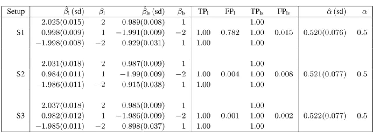
Setup βˆl(sd) βl βˆls(sd) βls TPl FPl TPls FPls αˆ(sd) α 2.025(0.015) 2 0.989(0.008) 1 1.00 S1 0.998(0.009) 1 −1.991(0.009) −2 1.00 0.782 1.00 0.015 0.520(0.076) 0.5 −1.998(0.008) −2 0.929(0.031) 1 1.00 1.00 2.031(0.018) 2 0.987(0.009) 1 1.00 S2 0.984(0.011) 1 −1.99(0.009) −2 1.00 0.004 1.00 0.008 0.521(0.077) 0.5 −1.986(0.011) −2 0.915(0.038) 1 1.00 1.00 2.037(0.018) 2 0.985(0.009) 1 1.00 S3 0.982(0.012) 1 −1.986(0.009) −2 1.00 0.001 1.00 0.002 0.522(0.077) 0.5 −1.985(0.011) −2 0.898(0.037) 1 1.00 1.00
Table 1 Estimates for the coefficients and selection proportions of the variables in the three simulation setups for100simulation runs. Estimates of coefficients from informative variables are displayed individ-ually and coefficients corresponding to non-informative variables in an overall average. TP stands for true positive and indicates the percentage, with which the informative variables were selected for each variable individually. Intercepts are in the model automatically, hence no selection frequency is reported. FP stands for false positive and denotes the over all percentage of selected non-informative variables per model.
setups were chosen to give insight in all three questions. We will first describe the basis for all three models and then point out the differences in the simulation concepts. All three models are based on the following sub-predictors:
ηlij =x>lijβl and ηlsij =xls>iβls+βttij+γ0i+γ1itij.
The matricesXlandXlsare the collections of the standardised covariates,βl= (2,1,−2,0)>andβls= (1,−2,0)> the corresponding linear effects with sub vectors0of different lengths,βt = 1is the impact
of timet,γ0the random intercept andγ1the random slope. In all three setupsN = 500individuals were
generated. For each individual, we drew five time points which were reduced to less than five in cases with events before the last observation. If there was no incident for any of the simulated individuals the number of observations would thus be2500. However the simulations are constructed in a way that this case never occurs. The first of the three setups (S1) was constructed to mimic the data situation of the application in Section 4 more closely and to thus better demonstrate the ability of the algorithm to perform variable selection in a lower dimension. S1 had four non informative covariates in each predictor. In the second simulation setup (S2) we used600non informative covariates,300for each sub-predictor. In this case the number of covariates exceeds the number of individuals. In the third of the three setups (S3) we chose the number of non informative covariates to be2500over both sub-predictors, i.e. 1250each, the theoretical maximum number of observations is hence exceeded by the number of covariates. Please note that we first simulated a genuine informative part of the model, and afterwards drew the non informative covariates for each setup individually. The three setups are hence based on the same data and the informative covariates of the three models are the same. In all three setups the association parameter was chosen to be0.5.
3.2 Results
We ran100models of each setup; results are summarized in Table 1 and will be described in detail in the following.
S1 S2 S3
ηl 160.2 187.8 187.2
ηls 154.8 48.6 30.6
Table 2 Median, minimum and maximum number of stopping iterations for all three simulation setups listed separately for the two different sub-predictors.
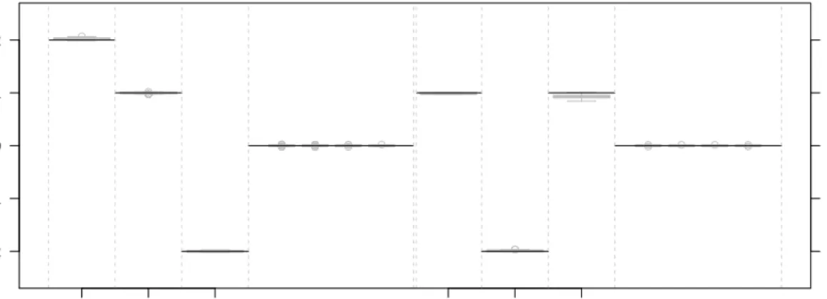
(i) Evaluation of estimation accuracy As can be seen in Table 1 estimation for the coefficients of the sub-predictors were very close to the true values. Standard deviations were small, except for the estimation of the time effect, where the variation between the simulation runs is slightly higher. A graphical illustration is provided in Figure 1, which displays boxplots of the resulting coefficients for S3 (the results for the other setups only differs slightly). The slight tendency of underestimation can be attributed to the shrinkage behavior of boosting algorithms in general. This underestimation can be observed in all three models in both parts. The estimation of the crucial association parameterαwas also very close to the true value in all setups (see the last column of Table 1 and Figure 2). The slight tendency to overestimateαcan be contributed to the compensatory behaviour of the association parameter. This is due to the fact thatαis estimated via optimisation and hence not subject so shrinkage but adapting directly to the data.
(ii) Variable selection properties All informative variables were selected in100% of the runs in all three setups. In S1, more non-informative variables (76.8%) were selected in the longitudinal predictor than in the shared predictor (1.5%). Boosting tends to select a higher percentage of non-informative variables in a small setup, which explains the high selection rate in the longitudinal component. The fact that the shared part is less prone to this greedy behaviour of the algorithm can be contributed to the option to chose the random effect over one of the non-informative variables. In the high-dimensional setups non-informative effects are selected in very few of the runs in both setups. The longitudinal sub-predictor does even better than the shared sub-predictor in this case. There are slight differences, which can be attributed to the smaller number of runs it required(see paragraph below). Overall the selection property works very well for both parts of the model, especially in high-dimensional scenarios.
(iii) Stopping iterations The two (possibly different) stopping iterationsmstop,landmstop,lswere selected by evaluating the models run on adaptively adjusted10×10grids on an evaluation data set with1000 in-dividuals. In all setups the grid ran through a sequence from30to300in both directions – formstop,land
mstop,ls. Based on these results, in setup S2 and S3 it was consequently adapted such thatmstop,lwas cho-sen from an equally spaced sequence from95to140, while the grid formstop,lsran from130to220. The optimal stopping iterations were chosen such that the joint log likelihood was maximal on the patients left out of the fitting process (predictive risk). For an overview over the resulting stopping iterations see Table 2.
4
Cystic Fibrosis data
Cystic fibrosis is the most common life-limiting inherited disease among Caucasian populations, with most patients dying prematurely from respiratory failure. Children with cystic fibrosis in the UK are usually diagnosed in the first year of life, and subsequently require intensive support from family and healthcare services (Taylor-Robinson et al., 2013). Though cystic fibrosis affects other organs such as the pancreas and liver, it is the lung function that is of most concern, with gradual decline in function for most patients leading to the necessity of lung transplantation for many. Lung function decline in cystic fibrosis is accelerated if patients become infected with a range of infections (Qvist et al., 2015). However, the direction of causation is unclear. It may also be the case that accelerated lung function decline predisposes
● ● ● ● ● ● ● ● ● ● ● ● ● ● ● ●●●●●●●● ●●● ● ● ● ● ● ● ● ●● −2 −1 0 1 2 −2 −1 0 1 2 2 1 −2 0 1 −2 1 0 βl βls
Figure 1 Boxplot representing the empirical distribution of the resulting coefficients for simulation set-ting S1 over 100 simulation runs: on the left side coefficients for the longitudinal sub-predictor are dis-played, on the right side coefficients for the shared sub-predictor. The black solid lines indicate the true values. The narrow boxes display the estimation for the effects of the non-informative variables
● ● ● α S1 S2 S3 0.0 0.2 0.4 0.6 0.8 1.0
Figure 2 Boxplot of the resulting estimates of the association parameterαover all three simulation setups and 100 simulation runs. The black solid lines indicate the true parameter.
patients to risk of lung infection. There is thus utility in analyzing lung function decline, and time to lung infection in a joint model in order to gain more insight in the structure of the process.
We analyzed part of a dataset from the Danish cystic fibrosis registry. To achieve comparability between patients we chose to use one observation per patient per year. Lung function, measured in forced expiratory
0 100 200 300 400 −0.6 −0.4 −0.2 0.0 0.2 0.4 0.6 Iterations βl Height Weight Infection Diabetes 0 5 10 15 20 25 30 −2.0 −1.5 −1.0 −0.5 0.0 Iterations βls Age Pancreatic Insufficiency Age of Diagnosis Sex
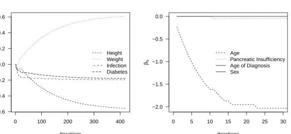
Figure 3 Coefficient paths for the fixed effects in the cystic fibrosis model. The graph on the left shows the coefficient paths for the longitudinal sub-predictor (displaying the influence on to the patients lung function), the graph on the right the coefficient paths of the shared sub-predictor (incorporated both in the longitudinal model for the lung function and the survival model for the Pseudomonas infection).
volume in one second (FEV1), is the longitudinal outcome of our joint model. The event in the survival part of the model is the onset of the pulmonary infectionPseudomonas aeruginosa(PA). After selecting the patients that have at least two observations before the infection, the data set contained a total of5425 observations of 417 patients of which48were infected with PA in the course of the study. The mean waiting time until infection was19.86, hence the mean age of infection was24.86years, since patients are included at the age of five into the study. The covariates for the longitudinal predictor were height and weight of the patient as well as two binary indicators: one states if the patient had one of three different additional lung infections and a second indicates if the patient had diabetes. The covariates possibly having an impact on the shared part of the model were time (i.e. age of the individuals), pancreatic insufficiency, sex, and age at which cystic fibrosis was diagnosed. Covariates were standardized to have mean zero and standard deviation one, except for age, which was normed on an interval from zero to one.
We then ran our boosting algorithm on the data set in order to simultaneously estimate and select the most influential variables for the two sub-predictors while optimizing the association parameter α. As recommended, we used a fixed step length of 0.1 for both predictors and optimizedmstop instead. The stopping iterations (mstop,l = 420andmstop,ls = 30) were chosen based on tenfold cross validation via a two-dimensional 15×15grid, sequencing in equidistant steps of 30 from 30to 450. The resulting coefficient paths for both sub-predictors are displayed in Figure 3.
The selected variables chosen to be informative for the joint model wereheight,weight,(additional) infec-tion,age,pancreatic insufficiencyanddiabetes.Age of diagnosisandsexdid not show to have an impact and were not selected. Being diabetic results to have a negative impact on the lung function, the same holds for having an additional lung infection or pancreatic insufficiency. The negative impact ofageon the lung function was to be expected since lung function typically declines for patients getting older. The result-ing negative impact ofheightand the positive impact ofweightindicate, that following our joint model, underweight has a negative influence on the lung function.
The association parameter α is negative with a value of −0.520. The risk of being infected is hence implicitly – i.e. via the shared predictor – associated negatively with the value of the lung function. Lower
lung function thus leads to a higher risk of being infected with pseudomonas emphasizing the need to model both outcomes simultaneously in the framework of joint models.
5
Discussion and Outlook
Joint modelling is a powerful tool for analysing longitudinal and survival data, as documented by Rizopou-los (2012). It is increasingly applied in biomedical research, yet it was unfeasible for high-dimensional data and there have been no suggestions for automated variable selection until now. Statistical boosting on the other hand is a modern machine-learning method for variable selection and shrinkage in statistical models for potentially high-dimensional data. We present a possibility to merge these two state of the art statistical fields. Our suggested method leads to an automated selection of informative variables and can deal with high-dimensional data and, probably even more importantly, opens up a whole new range of possibilities in the field of joint modelling.
Boosting algorithms utilizing the underlying base-learners are very flexible when it comes to incorporating different types of effects in the final models. Due to the modular nature of boosting (B¨uhlmann et al., 2014), almost any base-learner can be included in any algorithm – although the regression setting defined by the underlying loss function might be extremely different. In our context, the proposed boosting algorithm for joint models could facilitate for the construction of joint models including not only linear effects and splines, but for example, also spatial and regional effects.
A second area in which the suggested model calls for extension is variable selection itself. While informa-tive variables are selected reliably in most cases, also non informainforma-tive variables are included in too many iterations. With this being a structural problem of boosting algorithms (B¨uhlmann and Yu, 2007) in low-dimensional settings, the solution could be stability selection (Meinshausen and B¨uhlmann, 2010; Shah and Samworth, 2013), as shown to be helpful in other cases (Hofner et al., 2015; Mayr et al., 2016). The difference in the proportion of falsely selected variables between longitudinal and shared sub-predictor however, could be a joint modelling inherent problem and should be subject of future analysis. Further research is also warranted on theoretical insights, as it remains unclear if the existing findings on consis-tency of boosting algorithms (Zhang and Yu, 2005; B¨uhlmann, 2006) hold also for the adapted version for boosting joint models.
We plan to extend the model by incorporating a predictorηs, i.e. including covariates which only have an
impact on the survival time and are independent of the longitudinal structure. Once this is incorporated, we can make even better use of the features of boosting and implement variable selection and allocation between the predictors. The latter is especially useful if no prior knowledge on the structure of association exists, because covariates can be suggested for all three sub-predictors and the algorithm automatically assigns the informative covariates to the appropriate sub-predictor.
In conclusion we propose a new statistical inference scheme for joint models that also provides a starting point for a much wider framework of boosting joint models, covering a great range of potential models and types of predictor effects.
Acknowledgements
The work on this article was supported by the German Research Foundation (DFG), grant SCHM 2966/1-2, grant KN 922/4-2 and the Interdisciplinary Center for Clinical Research (IZKF) of the Friedrich-Alexander-University Erlangen-N¨urnberg (Projects J49 and J61). We furthermore want to thank the Editor and the reviewers, especially the one who saved us from falling into the trap of oversimplifying the gradient in our first draft of the algorithm.
A
Gradient of the shared predictor
In the following we will sketch out the calculus for the gradient of the likelihood of the shared sub-predictor, indices for individuals/obsevations (i.e. ij will be omitted. Note that the derivation of the first part in equation (4) with respect toηlsis the same as in the purely longitudinal predictor σ12(y−ηl−ηls). The additional part in the likelihood of the shared sub-predictor is simply the one of a pure survival model
f(T, δ|ηls, λ, α) = [λexp(αηls)] δ exp " −λ Z T 0 exp(αηls)dt # .
The formulation of the log likelihood is thus:
log (f(T, δ|ηls, λ, α)) = δlog(λ) +δαηls | {z } (l1) −λ Z T 0 exp(α(ηls))dt | {z } (l2) .
This again splits into two part (l1) and (l2). The derivation of the first part (l1) is straight forward and reduces to δα. The part of the likelihood less straight forward to differentiate is the part including the integral (l2) d dηls λ Z T 0 exp (αηls)dt.
Note thatηlsis a function of time such that standard derivation cannot be used. To avoid confusion with the upper integral boundT and the integration variable dtabove, we suppress the argument time in the following. Applying the rules for functional derivatives, we obtain
d dηls λ Z T 0 exp (αηls)dt=λ Z T 0 αexp (αηls)dt.
In the case of interest in this paper, where only the second part of the predictor is time-dependent, i.e.,
ηls=ηls−t+ (βt+γ1)t, the functional derivative of the functionηlshas the following form:
Z T 0 exp (α(ηls−t+ (βt+γ1)t))dt = α α(γ1+βt) exp(αηls−t+α(βt+γ1)t) T 0 = exp(αηls−t+α(βt+γ1)T)−exp(αηls−t) γ1+βt .
The whole derivation of the likelihood for the shared subpredictor hence is 1 σ2(y−ηl−ηls) +δα−λ exp(αηls)−exp(αηls−t) γ1+βt .
B
Simulation
• Choose a number of patientsNand a number of observationsniper patienti, i= 1, . . . , n
• Simulate the time points:
– drawn=N·nidays in1, . . . ,365
– generate the sequenceti of lengthniyears per patient, by taking the above simulated values as
– to make calculations easier, divide everything by 365
– example: time points for patientigiven thatni= 5:t= (.2,1.6,2.4,3.1,4.8)means the patient
was seen in the first year at day0.2·365, in year two at day0.6·365and so on
• Generate the longitudinal predictorηl
– generate fixed effects by choosing appropriate values for the covariate matrixXl – the covariate matrix can also include the time vector
– and deciding for values for the parameter vectorβl – calculateηl=Xlβl
• Generate the shared predictorηlsoutcomes based on the time points (just as in a usual longitudinal setup):
– generate random interceptγ0and random slopeγ1by drawing form a standard Gaussian
distri-bution
– generate fixed effects by choosing appropriate values for the covariate matrixXls(note that the values are not allowed to be time varying)
– and deciding for values for the parameter vectorβls – calculateηls=Xlsβls+γ0+γ1t
• drawnvalues ofyfromN(ηls(t) +ηl(t), σ2)
• Simulate event times (based on the above simulated times and random effects):
– choose a baseline hazardλ0 (for simplicity reasons chosen to be constant) and an association
parameterα
– calculate the probability of an event happening up to each time pointtijwith the formulaFtij = 1−exp−λ0
exp(α(ηls(t)))−exp(αηls−t) α(βt+γ1)
– drawnuniformly distributed variablesuij
– ifuij < Ftij consider an event having happened beforetij
– define time of eventsias proportional to the difference ofuijandFtij betweentijandtij−1 – for every individualionly the firstsiis being considered
– define the censoring vectorδof lengthN withδi = 0ifuij < Ftij for anyj = 1, . . . , niand
δi= 1otherwise (this leads to an average censoring rate of83.6%).
• for every individualidelete ally(tij)withtij≥sifrom the list of observations
The probabilities for the events are taken from the connection between the hazard rate and the survival function. F(t) = 1−S(t) = 1−exp(− Z t 0 λ(t))dt = 1−exp(−λ0 Z t 0 exp (αηls(t)) dt) = 1−exp −λ0 exp (αηls(t))−exp(αηls−t) α(βt+γ1)
References
Armero, C., A. Forte, H. Perpinan, M. J. Sanahuja, and S. Agusti (2016). Bayesian joint modeling for assessing the progression of chronic kidney disease in children.Statistical Methods in Medical Research online first, 1–17. Barrett, J., P. Diggle, R. Henderson, and D. Taylor-Robinson (2015). Joint modelling of repeated measurements
and time-to-event outcomes: flexible model specification and exact likelihood inference. Journal of the Royal Statistical Society: Series B (Statistical Methodology) 77(1), 131–148.
B¨uhlmann, P. (2006). Boosting for high-dimensional linear models.The Annals of Statistics 34(2), 559–583. B¨uhlmann, P., J. Gertheiss, S. Hieke, T. Kneib, S. Ma, M. Schumacher, G. Tutz, C. Wang, Z. Wang, and A. Ziegler
(2014). Discussion of ’The evolution of boosting algorithms’ and ’Extending statistical boosting’. Methods of Information in Medicine 53(6), 436–445.
B¨uhlmann, P. and T. Hothorn (2007). Boosting algorithms: Regularization, prediction and model fitting (with discus-sion).Statistical Science 22, 477–522.
B¨uhlmann, P. and B. Yu (2007). Sparse boosting.Journal of Machine Learning Research 7, 1001–1024.
Chan, J. S. K. (2016). Bayesian informative dropout model for longitudinal binary data with random effects using conditional and joint modeling approaches.Biometrical Journal 58(3), 549–569.
Efendi, A., G. Molenberghs, E. Njagi, and P. Dendale (2013). A joint model for longitudinal continuous and time-to-event outcomes with direct marginal interpretation.Biometrical Journal 55(4), 572–588.
Fieuws, S. and G. Verbeke (2004). Joint modelling of multivariate longitudinal profiles: pitfalls of the random-effects approach.Statistics in Medicine 23, 3093–3104.
Freund, Y. and R. Schapire (1996). Experiments with a new boosting algorithm. InProceedings of the Thirteenth International Conference on Machine Learning Theory, San Francisco, CA, pp. 148–156. San Francisco: Morgan Kaufmann Publishers Inc.
Friedman, J. H. (2001). Greedy function approximation: A gradient boosting machine. The Annals of Statistics 29, 1189–1232.
Friedman, J. H., T. Hastie, and R. Tibshirani (2000). Additive logistic regression: A statistical view of boosting (with discussion).The Annals of Statistics 28, 337–407.
Gao, S. (2004). A shared random effect parameter approach for longitudinal dementia data with non-ignorable missing data.Statistics in Medicine 23, 211–219.
Guo, X. and B. P. Carlin (2004). Separate and joint modeling of longitudinal and event time data using standard computer packages.The American Statistician 58, 16–24.
Ha, I. D., T. Park, and Y. Lee (2003). Joint modelling of repeated measures and survival time data. Biometrical Journal 45(6), 647–658.
Hepp, T., M. Schmid, O. Gefeller, E. Waldmann, and A. Mayr (2016). Approaches to regularized regression–a com-parison between gradient boosting and the lasso.Methods of Information in Medicine 55(5), 422–430.
Hofner, B., L. Boccuto, and B. G¨oker (2015). Controlling false discoveries in high-dimensional situations: Boosting with stability selection.BMC Bioinformatics 16(144).
Hofner, B., A. Mayr, N. Robinzonov, and M. Schmid (2014). Model-based boosting in R: a hands-on tutorial using the R package mboost.Computational Statistics 29(1-2), 3–35.
Hofner, B., A. Mayr, and M. Schmid (2016). gamboostLSS: An R package for model building and variable selection in the GAMLSS framework. Journal of Statistical Software 74(1), 1–31.
Li, N., R. M. Elashoff, and G. Li (2009). Robust joint modeling of longitudinal measurements and competing risks failure time data. Biometrical Journal 51(1), 19–30.
Liu, L., R. A. Wolfe, and J. D. Kalbfleisch (2007). A shared random effects model for censored medical costs and mortality.Statistics in Medicine 26, 139–155.
Mayr, A., H. Binder, O. Gefeller, and M. Schmid (2014a). The evolution of boosting algorithms - from machine learning to statistical modelling.Methods of Information in Medicine 53(6), 419–427.
Mayr, A., H. Binder, O. Gefeller, and M. Schmid (2014b). Extending statistical boosting - an overview of recent methodological developments.Methods of Information in Medicine 53(6), 428–435.
Mayr, A., N. Fenske, B. Hofner, T. Kneib, and M. Schmid (2012). Generalized additive models for location, scale and shape for high-dimensional data – a flexible aproach based on boosting.Journal of the Royal Statistical Society: Series C (Applied Statistics) 61(3), 403–427.
Mayr, A., B. Hofner, and M. Schmid (2012). The importance of knowing when to stop. Methods of Information in Medicine 51(2), 178–186.
Mayr, A., B. Hofner, and M. Schmid (2016). Boosting the discriminatory power of sparse survival models via opti-mization of the concordance index and stability selection. BMC Bioinformatics 17(288). doi: 10.1186/s12859-016-1149-8.
Meinshausen, N. and P. B¨uhlmann (2010). Stability selection (with discussion). Journal of the Royal Statistical Society. Series B 72, 417–473.
Qvist, T., D. Taylor-Robinson, E. Waldmann, H. Olesen, C. Rø nne Hansen, M. I. Mathiesen, N. Hø iby, T. L. Katzen-stein, R. L. Smyth, D. P., and P. T (2015). Infection and lung function decline; comparing the harmful effects of cystic fibrosis pathogen. in press.
Rigby, R. A. and D. M. Stasinopoulos (2005). Generalized additive models for location, scale and shape. Journal of the Royal Statistical Society: Series C (Applied Statistics) 54(3), 507–554.
Rizopoulos, D. (2010). JM: An R package for the joint modelling of longitudinal and time-to-event data. Journal of Statistical Software 35(9), 1–33.
Rizopoulos, D. (2012). Joint Models for Longitudinal and Time-to-Event Data: With Applications in R. Chapman & Hall/CRC Biostatistics Series. Taylor & Francis.
Schmid, M. and T. Hothorn (2008). Boosting additive models using component-wise P-splines.Computational Statis-tics & Data Analysis 53, 298–311.
Schmid, M., S. Potapov, A. Pfahlberg, and T. Hothorn (2010). Estimation and regularization techniques for regression models with multidimensional prediction functions.Statistics and Computing 20, 139–150.
Shah, R. D. and R. J. Samworth (2013). Variable selection with error control: Another look at stability selection. Journal of the Royal Statistical Society: Series B (Statistical Methodology) 75(1), 55–80.
Sweeting, M. J. and S. G. Thompson (2011). Joint modelling of longitudinal and time-to-event data with application to predicting abdominal aortic aneurysm growth and rupture.Biometrical Journal 53(5), 750–763.
Taylor-Robinson, D., R. L. Smyth, P. Diggle, and M. Whitehead (2013). The effect of social deprivation on clinical outcomes and the use of treatments in the uk cystic fibrosis population: A longitudinal study. Lancet Respir Med 1, 121–128.
Taylor-Robinson, D., M. Whitehead, F. Diderichsen, H. V. Olesen, T. Pressler, R. L. Smyth, and P. Diggle (2012). Understanding the natural progression in with cystic fibrosis: a longitudinal study.Thorax 67, 860–866. Tsiatis, A. and M. Davidian (2004). Joint modelling of longitudinal and time-to-event data: an overview. Statistica
Sinica 14, 809–834.
Tutz, G. and H. Binder (2006). Generalized additive modeling with implicit variable selection by likelihood-based boosting.Biometrics 62, 961–971.
Wulfsohn, M. and A. Tsiatis (1997). A joint model for survival and longitudinal data measured with error. Biomet-rics 53, 330–339.
Zhang, T. and B. Yu (2005). Boosting with early stopping: convergence and consistency. Annals of Statistics, 1538– 1579.