Statistical Inference Utilizing Agent Based Models

(1)

Statistical Inference Utilizing Agent Based Models

by

Daniel Heard

Department of Statistical Science Duke University

Date:

Approved:

David Banks, Supervisor

Sayan Mukherjee

Jim Berger

Jim Moody

Dissertation submitted in partial fulfillment of the requirements for the degree of Doctor of Philosophy in the Department of Statistical Science

in the Graduate School of Duke University 2014

(2)

Abstract

Statistical Inference Utilizing Agent Based Models

by

Daniel Heard

Department of Statistical Science Duke University

Date:

Approved:

David Banks, Supervisor

Sayan Mukherjee

Jim Berger

Jim Moody

An abstract of a dissertation submitted in partial fulfillment of the requirements for the degree of Doctor of Philosophy in the Department of Statistical Science

in the Graduate School of Duke University 2014

(3)

Copyright c 2014 by Daniel Heard

(4)

Abstract

Agent-based models (ABMs) are computational models used to simulate the behav-iors, actions and interactions of agents within a system. The individual agents each have their own set of assigned attributes and rules, which determine their behavior within the ABM system. These rules can be deterministic or probabilistic, allowing for a great deal of flexibility. ABMs allow us to observe how the behaviors of the individual agents affect the system as a whole and if any emergent structure develops within the system. Examining rule sets in conjunction with corresponding emergent structure shows how small-scale changes can affect large-scale outcomes within the system. Thus, we can better understand and predict the development and evolution of systems of interest.

ABMs have become ubiquitous—they used in business (virtual auctions to select electronic ads for display), atomospheric science (weather forecasting), and public health (to model epidemics). But there is limited understanding of the statistical properties of ABMs. Specifically, there are no formal procedures for calculating confidence intervals on predictions, nor for assessing goodness-of-fit, nor for testing whether a specific parameter (rule) is needed in an ABM. Motivated by important challenges of this sort, this dissertation focuses on developing methodology for uncer-tainty quantification and statistical inference in a likelihood-free context for ABMs. Chapter 2 of the thesis develops theory related to ABMs, including procedures for model validation, assessing model equivalence and measuring model complexity.

(5)

Chapters 3 and 4 of the thesis focus on two approaches for performing likelihood-free inference involving ABMs, which is necessary because of the intractability of the likelihood function due to the variety of input rules and the complexity of out-puts. Chapter 3 explores the use of Gaussian Process emulators in conjunction with ABMs to perform statistical inference. This draws upon a wealth of research on emulators, which find smooth functions on lower-dimensional Euclidean spaces that approximate the ABM. Emulator methods combine observed data with output from ABM simulations, using these to fit and calibrate Gaussian-process approximations. Chapter 4 discusses Approximate Bayesian Computation for ABM inference, the goal of which is to obtain approximation of the posterior distribution of some set of parameters given some observed data.

The final chapters of the thesis demonstrates the approaches for inference in two applications. Chapter 5 presents models for the spread of HIV based on detailed data on a social network of men who have sex with men (MSM) in southern India. Use of an ABM allows us to determine which social/economic/policy factors contribute to the transmission of the disease. We aim to estimate the effect that proposed medical interventions will have on the spread of HIV in this community. Chapter 6 examines the function of a heroin market in the Denver, Colorado metropolitan area. Extending an ABM developed from ethnographic research, we explore a procedure for reducing the model, as well as estimating posterior distributions of important quantities based on simulations.

(6)

(7)

List of Tables

2.1 Eigenvalues and γ coefficients for the 48 principal components of the Greenhouse model and indications of the components retained for val-ues ofγ0. Adjusted R2 is given for the four regression models to

mea-sure goodness-of-fit (adjusted R2 _{for regression using all 48 principal}

components is 0.863). . . 30 2.2 Original inputs which were identified as relevant with respect to total

greenhouse production using forward identification (F) and backward elimination (B) methods, for values ofγ0 p0.2,0.1,0.05,0.1q. Bullets

() indicate variables identifed as relevant and dashes (-) indicate irrel-evant variables. A description of the inputs can be found in Kasmire et al. (2013). . . 32 5.1 Estimated rates of interaction within and across blocks from the MMSB. 88 5.2 MMSB assignments compared to marital status . . . 89 6.1 Averages of quantities of interest for the heroin market model by time

step. The averages show clear divergence from the 1 minute values as the time step increases. . . 101 6.2 Compression-ratio complexity measures for full and reduced versions

(12)

List of Figures

1.1 The elements of the ODD protocol. The three categories on the left serve to explain the general structure of the protocol, not to describe the model. Model description following ODD protocol consists of the

the seven elements on the right. . . 3

2.1 Map of Michigan population density by county with blue diamonds representing locations of the four facilities receiving contaminated Methylprednisolone Acetate. . . 9

2.2 Comparison of simulated fungal meningitis case counts from (a) the FMO model and (b) the Zechman model from October 2012 through August 2013 based on 100 simulations from each model. Red points represent actual case counts from the outbreak. . . 15

2.3 An illustration of equivalence in mean modulo monotonicity. . . 18

2.4 An illustration of topological equivalence of maps. . . 21

2.5 An illustration of equivalence in mean modulo monotonicity. . . 22

2.6 An illustration of containment of input spaces. . . 23

2.7 An illustration of disjoint input spaces. . . 24

3.1 Diagram (left) and graphical (right) representations of arbitrary splits on the first dimension of a 2-dimensional input space, X, along with the corresponding swap and rotate operations. 3.1(a) shows the tree, 3.1(b) shows how the swap operation leaves an empty node, and 3.1(c) shows the rotate operation. . . 51

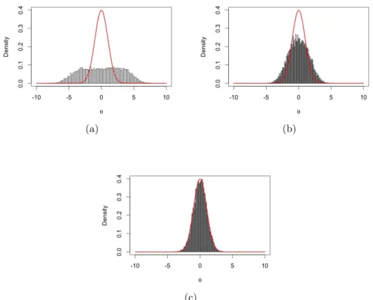
4.1 Histograms of the approximate posterior from ABC in the normal example with 5 (a), 2 (b), and 0.1 (c). In each plot, the red line represents the true posterior density. . . 72

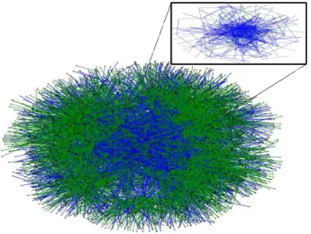
5.1 MSM Network Visualization. Inset represents edges restricted to the 245 egos. . . 83

(13)

5.2 Variational inference algorithm for variational free parameters, with lower panel corresponding to the nested algorithm for inference for (φqÑp, φqÐp) . . . 88 5.3 Approximate log-likelihood of MMSB by number of latent blocks . . . 89 5.4 Posterior membership vectors~πp for egos . . . 89 5.5 Comparisons of goodness-of-fit measures of the actual network (red

line) to 500 simulations of the ABM. Figure 5.5(a) shows the degree distribution of the network, Figure 5.5(b) shows the distribution of edgewise-shared partnerships and Figure 5.5(c) shows the distribution of minimum geodesic distances. The vertical axis for all of the plots are on the log-odds scale. . . 91 5.6 Output from 50 simulations of the MSM network ABM. Red bars

represent 95% confidence intervals for community HIV rate based on Armbruster et al. (2013). . . 94 5.7 Principal component basis for MSM network ABM (a) and

kernel-based discrepancy basis (b). . . 94 5.8 Two-dimensional marginals for the posterior distribution of theθ

pa-rameters. . . 95 5.9 Top: posterior 95% credible interval for the calibrated ABM,ηpx1, θq.

Middle: posterior 95% credible interval for the discrepancy function,

δpx1q. Bottom: posterior 95% credible interval for prediction of the

network trajectory, ξpx1, θq ηpx1, θq δpx1q. . . 97

6.1 Plots of quantities of interest for the heroin market versus log time step.101 6.2 Histograms of populations 1 (top row) through 5 (bottom row;

ap-proximation of posterior distribution) of Θ ppo, pa, pdq from ABC SMC approach with T 5 populations. Red lines indicate means from simulations of the full model. . . 105 A.1 Map of states with facilities which received contaminated

Methylpred-nisolone Acetate (PF) . . . 110 A.2 Map of case counts by state for the 2012-2013 fungal meningitis outbreak111 B.1 Comparison of summary statistics for full and reduced versions of the

IDMS model. Dashed lines represent 2.5% and 97.5% output quantiles.112 B.2 Adjusted p-values on negative-log scale for each of the four summary

(14)

List of Abbreviations and Symbols

Symbols

diag pq A diagnoal matrix.

Epq Expected value of a random variable.

Npµ, σ2q _{A univariate normal distribution with mean} _µ_{and variance} _σ2_.

Nppµ,Σq A p-dimensional normal distribution with meanµand covariance matrix Σ.

Abbreviations

ABC Approximate Bayesian Computation. ABM Agent Based Model(ling).

CANDID Cell-phone Assisted Network Detection and Identification. FMO Fungal Meningitis outbreak.

GASP Gaussian Process Response Surface. IDMS Illicit Drug Market Simulation.

MMSB Mixed membership stochastic block model. MSM Men who have sex with men.

PCA Principal Components analysis. SVD Singular Value Decomposition.

(15)

Acknowledgements

I would like to begin by thanking my parents, Margaret and Dupree Heard, and my brother, Peter, for your unwavering faith in me and for setting a positive example which I have striven to emulate. Thank you to my incredible wife, Veronica, for your support, hard work and sacrifices to help me be successful, and for being an amazing mother to Monica.

Thank you to my friends Shaun, Wakashan, Marc, Percy, Cory, Austyn, David, Delrik, Kody and others who, in one way or another, assisted me along my journey. I want to thank the Department of Statistical Science at Duke for giving me the opportunity to study here. Thank you to David Banks, my thesis advisor and

consigliere whose suggestions and advice were invaluable during this process. Thank you to Sayan Mukherjee, Jim Berger and Jim Moody for serving on my committee and asking thought-provoking questions to cause me a healthy amount of discomfort. Thank you Karen, Nikki and Anne for always making sure my paperwork was taken care of. Thank you to Georgiy Bobashev, Joey Morris and RTI International for the research opportunity and financial support. Thanks to the other DSS students who have accompanied me during my study, both to celebrate and commiserate with me: Tim, Tsuyoshi, Tommy, Nick, Mary Beth, Thais and Maria.

If I have made any contribution, either to the academic community or to the world at large, then, to paraphrase Malcolm X, all of the credit is due to God. Only the mistakes have been mine.

(16)

1

Introduction

1.1 Overview

Many methods exist for studying the development of systems. Often, these systems are quite complex, making it difficult to understand functions of agents within the system and their effects on the system as a whole. Agent Based Models (ABMs) are computational models used to simulate the behaviors, actions and interactions of agents (individuals or collective entities) within a system. The individual agents are autonomous, having their own set of rules which determines their behavior and how they develop within the system. These models allow us to observe how the si-multaneous behaviors of individual agents affect the system as a whole and examine the resulting emergent structure. Thus, we can better understand and predict the evolution of systems of interest and the appearance of complex phenomena. In par-ticular, ABMs are becoming a valuable tool for simulating and better understanding human systems (Bonabeau, 2002).

Three of the earliest examples of ABMs include von Neumann machines or cellular automata (Kemeny, 1955); John Conway’s Game of Life (Gardner, 1970), which looked at the evoluation of a universe determined by its initial state in which cells

(17)

interact with one another; and Thomas Schnelling’s study of segregation (Schnelling, 1971). ABMs grew in popularity in the 1990s because of the ease of implementation that came with improvement of available computer technology. Social sciences began using ABMs to explore social phemomena over time and the growth of societies over time, notably Epstein and Axtell (1996). ABMs have been compared to other modelling approaches in various problem settings, e.g., Hooten and Wikle (2010). ABMs can be implemented in a wide variety of software, ranging from traditional statistical software to dedicated ABM simulation platforms (Railsback et al., 2006).

1.2 ODD Protocol

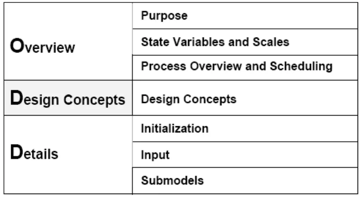
The ABM development process became more standardized with the publication of the ODD (Overview, Design concepts, and Details) Procotol by Grimm et al. (2006). This protocol is intended to make model descriptions more complete and more easily understood, primarily for academic literature. This, in turn, enables reproducbility of ABMs and addresses major concerns previously associated with ABMs (Lorek and Sonnenschein, 1999). An extensive discussion of ODD protocol can be found in Polhill et al. (2008), and a discussion of the growing use of the protocol is presented in Grimm et al. (2010). The protocol’s basic structure is presented in Figure 1.2.

The ‘Purpose’ section explains what the model is intended to do and its general goals. The ‘State Variables and Scales’ section outlines the structure of the model, identifying all of the entities in the model, such as types of agents, spatial structure and other local and global variables. Additionally, the variables that determine the state of these entities at any given point during the simulation are specified. The ‘Process Overview and Scheduling’ section lists all processes that occur in the model and in what order they occur. This covers the hierarchy of agent behaviors, effects on the environment and associated updates to states of model entities. The ‘Design Concepts’ section describes the general concepts upon which the model is based.

(18)

Figure 1.1: The elements of the ODD protocol. The three categories on the left

serve to explain the general structure of the protocol, not to describe the model. Model description following ODD protocol consists of the the seven elements on the right.

This is primarily to provide an understanding of why certain design decisions were made. Such concepts include a summary of emergent behavior, agent objectives, agent interactions and a description of agents’ perceptions and thought processes, if any exist. The ‘Initialization’ section identifies how the model is started and often provides references to support initial values of variables. The ‘Input’ section describes any other external inputs to the model (such as time-series market data in financial models or temperature data for a climate model). The ‘Submodels’ section explains in detail the equations and algorithms used in the model, as well as defining any parameters included in the model.

While ABMs are becoming ubiquitous, there is still a good deal of theory that re-mains to be developed. In particular, there has yet to be a standard model validation protocol specifically for ABMs, taking into account the multiple levels of behavior being simulated. Additionally, there is a lack of theory regarding the rigorous com-parison of two ABMs, specifically in the context of model equivalence and model complexity.

(19)

1.3 Approaches for Inference using ABMs

ABMs are of particular interest in statistics because we can use the inputs and outputs from these models as data to study complex relationships and, in a Bayesian context, perform statistical inference. Because of the variety of input rules and the complexity of outputs, the likelihood function for realistic ABMs is intractable; thus, any inference involving these models must be likelihood-free. The two likelihood-free methods of utilizing Agent Based models for statistical inference are emulation and Approximate Bayesian Computation (ABC).

1.3.1 Gaussian Process Emulators

Gaussian Process emulation deals with developing statistical models to approximate complex computer model output. This Bayesian approach has been implemented and studied widely, with some of the earliest work done by Anthony O’Hagan (1978) and Jerome Sacks et al. (1989). Recent advances have been made in the development and implementation of Bayesian computer model emulators (Lopes, 2011).

In many application of ABMs, the sophistication of the system being modeled leads to a complex model with detailed sets of agent rules. This model copmlexity can, naturally, lead to computationally burdensome simulations. As the number of ABM parameters grows, emulation becomes more useful, allowing ABM outcomes of interest to be predicted at settings without running the model at these settings. After specifying the set of parameters for the ABM and running it for a fixed set of inputs, a Gaussian Process Response Surface (GASP) will be fit to the ABM. The use of a Gaussian Pricess gives flexibility in modeling realizations which can be used to interpolate data points and make probability statements. Many variations on Gaussian Process emulation have been made which allow for their implementation in a broader class of problems with fewer assumptions needed.

(20)

1.3.2 Approximate Bayesian Computation

Approximate Bayesian Computation (ABC) is a class of methods that allows for approximate computation in the analysis of complex models. For problems in which the likelihood function is intractable (such as ABMs) or very expensive to compute, ABC allows us to perform statistical inference by simulating from an approximation to the posterior distribution. The approach involves sampling a parameter setθfrom a prior distrubition and generating datayconditional on the sampled parameters. If the generated data is close enough (according to some appropriate distance metric) to the observed data, then the sampledθis accepted as a draw from the posterior. Some of the earliest ABC methods were introduced by Tavare et al. (1997) and Pritchard et al. (1999) for applicatioins in genetics. Many extensions have been made since, such as Marjoram et al. (2003), Toni et al. (2009), Beaumont et al. (2009) and others. Further developments of ABC in complex dynamic systems (cf. Bonassi, 2013) are still being made. ABC has been applied to reinforcement learning problems (cf. Dimitrakakis and Tziortziotis, 2013), which deals with similar issues to those that arise with ABMs.

For ABMs, we can identify model parameters in which we are particularly in-terested. This will serve as the θ for which shall generate an approximate posterior distribution. This approach gives a straightforward method of inference about agent behaviors contributing to system development. This inference allows us to identify reasonable constraints on agent behavior in a more rigorous manner than previously possible.

1.4 Dissertation Outline

This dissertation analyzes multiple approaches for the development and implemen-tation of statistical inference utilizing ABMs. In chapter 2, I present theory which

(21)

addresses some of the areas related to ABMs which have not been thoroughly investi-gated. I propose a model validation protocol as well as examining methods for model comparison in terms of complexity and determining model equivalence. In chapter 3, I discuss the utility of Gaussian Process emulators for inference, examining multiple approaches for different problem settings. Chapter 4 analyzes Approximate Bayesian Computation techniques for assessing sets of parameters and rule sets for ABMs and performing posterior inference. Chapters 5 and 6 look at ABM applications which demonstrate both emulator and ABC techniques and examine the utility of ABMs in conjunction with other methods for analysis of HIV transmission in a network in southern India and the dynamics of a heroin market.

(22)

2

ABM Theory

2.1 Overview

ABMs are often used to simulate complex real world processes and in many cases are used for qualitative insight. A limitation in the use of ABMs has been the disconnect between existing theory, both in a mathematical sense and in the context of many theories of social behavior, discussed in detail in Chattoe (2003). To truly leverage ABMs and be able to explore ‘what if’ questions related to systems of interest, one must be precise in model specification to ensure it correctly simulates the system. Additionally, one should be able to quantitatively compare models for a given system based on various criteria in order to better understand system behavior and make determinations about the inclusion and treatment of model elements.

To this end, model validation is a crucial component in the development of ABMs. This procedure ensures that the dynamics being simulated in the model are a rea-sonable representation of the system and that the model itself is correctly capturing large-scale system behavior.

(23)

comparisons which it is important to be able to make. Identifying whether models are equivalent (in some sense) can be helpful in examining treatment of different variables and implementing the agent rule sets. Determining the relative complexity of two models can be a useful step in model selection for ABMs.

2.2 ABM Validation

Validating ABMs is an important component of model development. A general ap-proach for validation and verification of computer models is presented in chapter 3. Although validation of ABMs has some elements in common with validation of more traditional computer models, the process for ABMs is slightly different because the aggregate emergent structure must be considered in tandem with agent-level param-eters and rules. The Virtual Overlay Multi-Agnet System (VOMAS) verification and validation technique for ABMs is based in software engineering (Niazi et al., 2009). In this approach, a VOMAS is developed along with the ABM, in which the agents gather data through logs, providing run-time support of the validation process by checking for violations of user-specified settings. While the VOMAS approach is a thorough approach, it can become cumbersome in many cases, as it requires the de-velopment of two models. Some other work has been done exploring model validation strategies specifically for ABMs (Windrum et al., 2007; Fagiolo et al., 2007; Marks, 2012, 2013), however, it is very much an open problem.

Here, I propose a model validation protocol for ABMs and discuss it in relation to a model I developed for the multi-state fungal meningitis outbreak (FMO) of 2012-2013 within the state of Michigan (Centers for Disease Control & Prevention, 2013b).

In 2012, the New England Compounding Center (NECC) distributed contami-nated lots of Methylprednisolone Acetate for steriod injections to health care facilities in multiple states. Michigan had the highest incidence rate, with 264 cases and 19

(24)

deaths as of October 2013. A map of the facilities in the state is shown in Figure 2.2. Details of nationwide cases and facilities are presented in appendix A.

Figure 2.1: Map of Michigan population density by county with blue diamonds

rep-resenting locations of the four facilities receiving contaminated Methylprednisolone Acetate.

The output quantity of interest for this model is the number of cases of infection at a given time. We have data on the number of cases, taken at 52 time points between October 2012 and August 2013, as well as information on the specific products and quantities received by the facilities, as well as shipping dates from NECC which provide an estimate of when initial infections could have occured (US Food and Drug Administration, 2012).

2.2.1 Internal Validation

Internal validation involves examining components within the model in order to iden-tify potentially problematic areas, as well as to determine if the model is operating in a way that is consistent with the system it represents.

(25)

Step 1: Assess Face Validity

Assessing face validity of a model involves determining if the model’s structure and behavior are reasonable according to domain experts. This involves examination of rule sets for individual agents as well as the dynamics of the interactions of agents with each other and the system itself. Bharathy and Silverman (2010) and Xiang et al. (2005) discuss some specific techniques for evaluating model face validity. In the case of the heroin market ABM (discussed in chapter 6), the face validity of many of the model’s functions follows from the fact that it was developed from the ethnography of a domain expert.

For the FMO model, the central dymanic is the means by which the disease is spread. Here, the method by which agents contract the disease differs from traditional disease spread models because fungal meningitis is not contagious, as infection is only obtained through direct introduction into the blood stream. Thus, disease is passed from facilities to individual patients and not spread from patient to patient. While the locations of the facilities which received contaminated substances were identified, the number of cases for which the individual facilities were responsible was not identified. Demographic information for infected individuals (age, gender, race, etc.) was not provided either. To account for this, the affected facilities’ weekly visitor counts were determined in part by population density within 100 miles of each facility, based upon US Census estimates (US Census Bureau, 2013).

Additionally, an agent’s age influenced their probability of visiting one of the affected facilities, based on available information on visitor demographics in 2012 for similar facilities in the state (Michigan Headache & Neurological Institute, 2012). Out of 4606 annual visitors, 2.3% were age 6-17, 18.5% were age 18-40, 65.3% were age 41-65, 13.4% were age 66-85 and 0.5% were age 86 and older.

(26)

injection and contracting fungal meningitis was determined by an exponential model for modeling population growth (Brauer and Castillo-Chavez, 2012; Diekmann and Heesterbeek, 2000). The standardized observed case counts approximately fit the curve

Fpxq 1expp0.14x 0.08q

wherexis the week (with week 1 representing October 6, 2012). This model was cho-sen to capture the pattern of the outbreak, with decreasing numbers of case counts over time as the tainted materials are identified and removed. Because of the impor-tance of the time component in the outbreak, the above model was more appropriate for this application than a compartmental model (SIR, SEIR, etc.). This model fit well, with a sum of squared residuals over the first 14 weeks of 9.43. Differentiating this curve gives a function of the form of a scaled exponential distribution probability distribution function,

fpxq 0.14 expp0.14x 0.08q which can be normalized to give a proper pdf.

Because symptoms of infection were reported to appear 1 to 4 weeks after re-ceiving a contaminated injection (Centers for Disease Control & Prevention, 2013a), there is some uncertainty in the time between infection and case confirmation. To account for this and the lack of any additional information, based on the principle of maximum entropy, the time for an infected agent to be confirmed as a case was drawn from a discrete uniform (1,4).

A main emphasis of assessing face validity is understanding specific dynamics of the system being modeled and not merely beginning with an off-the-shelf model which may represent a system that functions quite differently from the system of

(27)

interest.

Step 2: Determine Evaluation Criteria

Output from ABMs can be complex and multidimensional. While all of the outputs may be related, it is possible that only a small subset are of primary interest when simulating the system. In the case of ABMs for networks, the are several different network measures (e.g. degree distribution) that could be of primary interest, but other associated values (e.g. density, clustering) are produced in the model output. Additionally, one should establish the range of inputs over which output evaluation is sought.

In the case of the FMO model, we are interested in the count of infections at time points throughout the simulation. We have data on case counts to which we will compare model simulation to evaluate the quality of the model’s representation of this outbreak. Because we have the relative proportion of patient visits by age to facilities similar to those affected in the outbreak, there is an estimate of on individual agent’s probability of visiting the facilities; but, because this is not exact, it is necessary to simulate behavior with a range of probabilities around these estimates.

2.2.2 External Validation

External validation involves comparing elements of the model to other sources. This component is significant in that it goes beyond determining the logical justifiability of the model to obtain a quantitative determination of how well the ABM represents the system.

Step 3: Output Analysis

The general strategy for external validation is the analysis of some output quantity. This approach can be separated into a number of more specific techniques which are discussed below.

(28)

Predictive Validation

In cases where longitudinal data is available, it is possible to develop the model using data only up to a certain time point, and then forward simulations can be checked against the subsequent data to determine the predictive accuracy of the model.

Because longitudinal data were available for the Meningitis outbreak, predictive validation was used for the FMO model. The model begins simulation in September 2012 and was built by fitting weekly data from October 2012 through December 2012 and then validated by comparing simulated case counts in the model to the observed case counts for January 2013 through October 2013. Case counts were provided at smaller time intervals in October 2012 when the outbreak was first identified, and then the intervals grew longer in December 2012, so some interpolation for case counts was necessary in the predictive validation. Because of the uncertainty in the time between infection and confirmation of fungal meningitis, as discussed earlier, the criterion for model agreement with the actual outbreak was the predicted model case counts falling within the range of observed case counts in a four week window.

Cross-model Validation

In many cases, different conceptual models can be used to simulate a particular phenomena. Cross-model validation leverages these instances and compares results of the ABM simulation to results from other models. This approach is useful in that it allows both qualitative and quantitative comparisons. In particular, when comparing a particular output quantity of an ABM to a different model which itself has been verified and validated, agreement of the two models strongly implies validation of the ABM. Axtell et al. (1996) discusses strategies for cross-model validation in detail.

When validating an ABM with another model which has already been validated, one may seek to assess equivalence between the models. Depending on the features of the respective models, there are different notions of equivalence which can be

(29)

considered. Some possible model equivalence measures are discussed in section 2.3. Regarding the fungal meningitis outbreak, while there were models developed to simulate the biological effects of the outbreak on individuals and treatment strategies (Pappas et al., 2013), there were no models developed specifically to simulate how the outbreak progressed. The closest validated model to which to compare the FMO model is an ABM for contamination events (Zechman, 2011).

The Zechman model was developed in AnyLogic (XJ Technologies, 2013) to sim-ulate response of indivudals to water contamination, incorporating a spatial compo-nent based on the proximity of individuals to the location of contamination, as well as timing and communcation which alters individuals’ water consumption and influ-ences change of use in response to the contamination. The simulation incorporates the EPANET water distribution system model (Shang et al., 2008).

By making adjustments to the Zechman model such as reducing the number of nodes (water sources) within the network, treating all nodes as commercial (to simulate a high number of visitors), and restricting the consumer demand at the nodes, the model’s operation closely resembles that of the FMO model. The Zechman model runs on a finer-scaled time step than the FMO model, which must also be taken into account. The simulations under the framework of the Zechman model give case counts consistent with those from the FMO model. While both models give average simulated case counts which capture actual case counts within a four week window, the Zechman model over-predicts cases early in the simulation (October 2012). A comparison of the simulation results is shown in Figure 2.2.

In addition to the comparison of the simulated case counts of the two models, the FMO model was found to be a less complex model than the Zechman model for the outbreak (see discussion of model complexity in section 2.4).

(30)

Weeks C ase s 1 3 5 7 9 11 1315 1719 2123 25 2729 3133 3537 3941 4345 0 25 50 75 100 125 150 175 200 225 250 275 (a) Weeks C ase s 1 3 5 7 9 11 1315 1719 2123 25 2729 3133 3537 3941 4345 0 25 50 75 100 125 150 175 200 225 250 275 (b)

Figure 2.2: Comparison of simulated fungal meningitis case counts from (a) the

FMO model and (b) the Zechman model from October 2012 through August 2013 based on 100 simulations from each model. Red points represent actual case counts from the outbreak.

(31)

Statistical Validation

Statistical validation is the most rigorous external validation method and can sig-nificantly increase the credibility of an ABM and can be performed in conjunction with predictive or cross-model validation. Hypothesis tests for equivalence of ABM output with either true system measurements or output of other models are a useful approach. Additionally, based on the data being used to validate the model, one can establish tolerance bounds for model output. These represent an acceptable range of model output values which can be considered to represent reasonable system behav-ior. One can then determine an acceptable proportion of output values which should fall within the tolerance bounds to evaluate model performance. Additionally, tol-erance bounds allow for varying degrees of accuracy in different model applications, as well as different degrees of uncertainty at different input settings. Discussion on applying statistical techniques to model validation in specific settings can be found in Kleijinen (1999) and Sanchez (2001).

A more rigorous and involved technique of statistical validation of ABMs involves approximating the model using Gaussian process techniques, as discussed in chapter 3.

Step 4: Feedback/feed forward

Model validation is very much an interative process, and the final step of the proce-dure involves using the findings of previous model validation steps to make adjust-ments to the model.

2.3 Model Equivalence

Given the variety of strategies for developing ABMs, one important topic to consider is that of model equivalence, as determined based upon some model output quantity. There has been some exploration of model equivalence related to model validation

(32)

in Robinson et al. (2005) and Yang et al. (2004), as well as discussion of the issues involving hypothesis testing as it relates to model equivalence in Welsh (1996) and Berger (2003) among others.

There are several topics to consider regarding separate models for a system and making comparisons among them. An important area which must be considered is that of the input sets/spaces of the models. These sets will fall into one of four possible categories: 1) The sets are the same, 2) There is partial overlap in the sets, 3) One set contains the other, 4) The sets are disjoint. The criteria for determining model equivalence is largely dependent upon the category into which the input sets fall.

When looking to assess model equivalence, there are three main types of equiva-lence one could seek to identify. We restrict the initial discussion of model equivaequiva-lence to the regions of the input space that both models have in common. We will dis-cuss the assessment of equivalence of two models, but the theory can be extended to consider larger collections of models.

For the subsequent discussion, let the two models be represented as maps f1 :

S1 Rp ÝÑ A1 R and f2 : S2 Rp ÝÑ A2 R. We begin by considering the

case where S1 S2 S and A1 A2 A.

Equivalence in mean

Two models are equivalent in mean if, given a fixed set of inputs, the mean functions of the output are equivalent. ABMs need not be deterministic, a fixed set of inputs can produce significant output variation from simulation to simulation for a given model. So, while exact equivalence (two models producing the exact same output for a fixed set of inputs) is rare in practice, equivalence in mean looks at the average of some output value of multiple simulations of the two models. Although the maps

(33)

space pΩ,F,Pq where Ω A, F is the Borel sets on A and, under the probability measure P, PpA Aq is the probability that a simulation run at input settings x0

will have an output value in A, which can be estimated based on a large-scale batch of simulations. We can consider the mean function to be the expected value of the simulation using the specified probability space.

Equivalence in mean modulo monotonicity

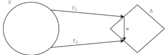
Equivalence in mean modulo monotonicity is a slightly relaxed version of equiva-lence in mean where, given two models, there exists a monotone (or anti-monotone) function m : A ÝÑ A such that mf1 f2. In this case, for a fixed set of inputs

xPS, there exists a monotone function which maps the mean function of one model to the mean function of the other model. The monotone function can be viewed as a calibration function.

Figure 2.3: An illustration of equivalence in mean modulo monotonicity.

As an example, consider two ABMs for weather forecasting, in which the agents are cubic kilometers of atmosphere and they interact by exchanging pressure, tem-perature and moisture. Model 1, for a fixed set of inputs, could have temtem-perature predictions of 65F, 70F and 75F, while model 2 could have temperature predic-tions of 80F, 85F and 90F. If this is the case for all sets of inputs, we can establish a monotone function mapping the output of model 1 to the output of model 2.

If the output space A_Ris connected, then we can consider this equivalence in an alternative way. By the connectedness of A, f1 and f2 are homotopic (i.e. there

(34)

exists a family of continuous functions ht : S Ñ A for t P r0,1s such that h0 f1

and h1 f2 and the map pS, tq ÞÝÑ htpq is continuous from S r0,1s to A.) One

can trivially define ht p1tqf1 tf2. If ht is monotone in t, then this homotopy formulation can serve as a surrogate for the m function discussed above.

Equivalence in distribution

Two models are equivalent in distribution if the distribution of the outputs is the same for the models given a fixed set of inputs. Equivalence in mean (or equivalence in mean modulo monotonicity) can be achieved by models which have outputs that differ greatly at each simulation. Consider again two weather forecasing ABMs. Model 1, for a fixed set of inputs, could have temperature predictions ranging between 65F and 75F, while model 2 could have temperature predictions ranging between 40F and 100F. While both would have the same mean, the variances differ greatly. The notion of equivalence in distribution takes variation of the outputs into con-sideration. While two models may not have outputs which match exactly, having the same distribution of outputs demonstrates a high-level agreement in the predicted behavior of the system. Certain tests for equivalence such as a Kolmogorov-Smirnov test and statistical measures such as Mahalanobis distance enable the assessment of equivalence in distribution. A detailed discussion of such tests is presented in Welleck (2010).

Theorem 1. (Topological Equivalence of Models) Let S _Rp _{be compact.} _Let

f1 :S ÝÑAR andf2 :S ÝÑAR be continuous maps, both of which represent

ABMs of a particular system. Supposef1 andf2 each have a finite number of critical

points (points where the derivative vanishes), denoted y1i andy2i, respectively (by the

compactness of S, this is equivalent to the critical points being isolated). The models

f1 and f2 are topologically equivalent if and only if the atoms of their critical values

(35)

For clarity, I define some terms before presenting a proof.

Two maps are topologically equivalent if there exist two homeomorphisms h : S ÝÑS and h1 :AÝÑA such that f1hh1f2.

Let f : S ÝÑ_R be a continuous map with a critical value c. If critical level set

f1_p_c_q_S _{contains only finitely many critical points, then a connected component}

Γ of f1pcqis called an atom of the critical value c of the function f.

Proof of Theorem 1: This proof closely follows work presented in Sharko (2003).

Necessity. Suppose f1 and f2 are topologically equivalent. Then there exists a

homeomorphism honS mapping the critical level sets of f1 to the critical level sets

of f2. The continuity of h ensures that connected components of the critical level

sets are mapped to each other. Hence, the atoms of the critical values of f1 and f2

are isomorphic.

Sufficiency. Let φ be an isomorphism between the atoms of the critical values of f1 and f2. By a theorem presented in Prishlyak (2002), because of the continuity

of the maps, each isolated critical point of f1 and f2 has a closed neighborhood in

which the map is topologically equivalent to a polynomial of the form xn c for some non-negative integer n and some constant c. Let Cripf1q and Cripf2q denote

these neighborhoods of the critical points. Following Sharko (2003), using φ, we can construct homeomorphismshi mappingCripf1qtoCripf2q. By Chapman (1972)

and Anderson (1967), we can extend the homeomorphisms hi to a homeomorphism

h1 defined on closed neighborhoods of curves that join critical points of f1, denoted

Uipf1q, and maps these neighborhoods toUipf2q, the corresponding neighborhoods of

the critical points off2.One can chooseh1in such a way that it maps the level curves

off1 inCripf1q YUipf1qto the level curves inCripf2q YUipf2q. By construction, the

closure of the complement ofpCripf1q YUipf1qq

pCripf2q YUipf2qqinS will consist

of the union of sets homeomorphic to cylinders (or hypercylinders depending on the dimension ofS), asCripf1qYUipf1qq

(36)

sets and any separated sets which make up this complement will be homeomorphic to (hyper-)cylinders (Salzmann, 1969). By Chapman (1972) and Anderson (1967), we can again extend the homeomorphism h1 to these (hyper-)cylinders so that the level

sets of f1 map to the level sets of f2. Identifying an appropriate homeomorphism h

on_R, we obtain topological equivalence off1 and f2.

With respect to the ABMs represented by f1 and f2, the conjugate

homeomor-phism h and h1 can be considered as a tuning function and a calibration function, respectively.

Figure 2.4: An illustration of topological equivalence of maps.

It is appropriate to note here that in the case where S1 S2 but, without loss

of generality, A1 A2, it follows that the model f1 is a proper subset of f2. In a

model selection scenario, this would make f2 a more favorable choice, unless there

were other issues, such as model complexity (discussed in section 2.4), that favored

f1. This case would then require some decision rule for a model selection.

2.3.1 Non-equivalent Input Spaces

The above discussion considered models for which the input spaces were the same. However, in many cases, different models for the same system may use different sets of inputs and have input spaces which are not the same. Here, we examine the three cases where S1 S2 and identify conditions for model equivalence in each of these

(37)

Intersection of Input Spaces

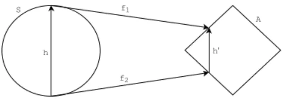
The first possible scenario for non-equivalent input spaces is the case where S1 and

S2 partially overlap so that there existx1 PS1zS2 andx2 PS2zS1 whileS1XS2 H.

Figure 2.5: An illustration of equivalence in mean modulo monotonicity.

In order to establish equivalence in mean, equivalence in mean modulo monotonic-ity, or equivalence in distribution of f1 and f2, one must first be able to establish a

homeomorphism h (tuning function) between S1 and S2. If this can be done, then

equivalence of each type can be determined as described in Section 2.2. If the home-omorphismh maps the atoms of the critical values off1 and f2 to one another, then

the models are topologically equivalent by Theorem 1. None of the forms of equiva-lence discussed above require the two models to have the same behavior on the set S1XS2.

If we look at the restrictions f1|S1_XS2 and f2|S1_XS1, it is possible to establish

equivalence of f1 and f2 on the set S1 XS2. For equivalence in mean, equivalence

in mean modulo monotonicity, and equivalence in distribution, one would only need to look at the behaviors of the maps restricted to this set. To establish topological equivalence on the set, one could look at the atoms of critical values of the restricted maps and, if they are isomorphic, then the maps are topologically equivalent when restricted to the intersection of the input spaces by Theorem 1. In we find f1|S1XS2

and f2|S1XS2 to be equivalent, then f1 and f2 are demonstrate partial equivalence.

(38)

are partially equivalent on S1 XS2, this can inform the nature of the discrepancy

between the two models.

Containment of Input Spaces

The second possible scenario for non-equivalent input spaces is the case where, with-out loss of generality, S1 S2.

Figure 2.6: An illustration of containment of input spaces.

In order to establish equivalence in mean, equivalence in mean modulo monotonic-ity, equivalence in distribution or topological equivalence for this case, the procedure is essentially the same as the case where S1 and S2 partially overlap.

If we look at the restriction f2|S1, it is possible to establish equivalence of f1

and f2 on S1. In we find f1 and f2|S1 to be equivalent, then f1 and f2 are partially

equivalent, as they are satisfy conditions for equivalence on the entire input space of

f1. If this is the case, the behavior of f2 on the set S2zS1 determines if the models

fully satisfy the conditions for equivalence.

If we find that f2pS2zS1q f2pS1q, then f2 is a more complex model in the

Kolmogorov sense thanf1 (see discussion of model complexity in section 2.4) and f1

is a more parsimonious representation of the system of interest.

If there exists yPf2pS2zS1q such thatyR f2pS1q, thenf2 is capable of capturing

(39)

Disjoint Input Spaces

The third possible scenario for non-equivalent input spaces is the case whereS1XS2

H.

Figure 2.7: An illustration of disjoint input spaces.

In order to establish equivalence in mean, equivalence in mean modulo monotonic-ity, equivalence in distribution or topological equivalence for this case, the procedure is essentially the same as the other cases of non-equivalent input spaces. In general, it is unlikely that two models with completely disjoint input spaces (i.e. having no inupt variables in common) will be equivalent.

For any set of non-equivalent input spaces, in the case whereS1 andS2 are of

dif-ferent dimensions (i.e. f1 has more input variables than f2), the two models cannot

be topologically equivalent, since one cannot establish a homeomorphism between S1 and S2. Letting S1 Rm and S2 Rn for m n, since S1 and S2 are simply

connected by construction, the (open) interiors of S1 and S2 are homeomorphic to

Rm andRn,respectively by the Riemann mapping theorem. As a result of invariance of domain (Brouwer, 1912) and the Jordan-Brouwer separation theorem (Alexander, 1922), _Rm _and

Rn are not homeomorphic. Hence, S1 and S2 cannot be

homeo-morphic, otherwise one could construct a homeomorphism between _Rm _and

Rn by composition.

(40)

2.4 Model Complexity

A related concept to model equivalence is that of model complexity. Some work has been done on quantifying the complexity of statistical models (Vanpaemel, 2009; Spiegelhalter et al., 2002), but there has been limited exploration of this topic as related to ABMs. A general discussion of the complexity of simulation models as well as advantages and disadvantages of increasing the level of detail of a simulation model is presented in Chwif et al. (2000). A major limitation at this point is that there is no widely accepted definition of what a complex model is, nor is there any general complexity measure of a given simulation model. When comparing two models, one may have an intuition as to when one model is more complex than another (specfically, this occurs when one creates a ‘reduced’ or ‘simplified’ version of an ABM, as described in chapter 6). In these cases and in less straightforward cases where two different models exist for the same system, having some metric for comparing the complexity of the models can be useful. Here, we propose two measures of complexity for simulation models.

A naive method for comparing model complexity is by comparing model run-time. For two models of a system with the same time step, the model which takes longer to simulate a fixed period of time is, in a sense, more complex than another.

The notion of Kolmogorov complexity (Gammerman and Vovk, 1999; Li and Vitaanyi, 2008) identifies the complexity of an object as the shortest program written in a fixed language which can produce the object. Given two models for a system in a particular language, one could use this concept to compare the complexity of two models using length of the programs. There is also the ability to incorporate an interpreter, which enables models to be translated between programming languages and, hence, the comparison of models in different languages.

(41)

Kolmogorov complexity of a model, which is useful for comparing the complexity of models for which the codes have similar structure.

A more formal approach for assessing model complexity is based in the infor-mation theoretic approach of model compression. Several compression algorithms exist, but the two most prominent lossless compression algorithms are Huffman cod-ing and Lempel-Ziv codcod-ing (Hufman, 1952; Ziv and Lempel, 1977, 1978). One can then use the compression ratio (uncompressed model size_{compressed model size} ) as a measure model complexity, as proposed by Khalatur et al. (2003) and Evans and Bush (2001). Considering model complexity in this way, the model with a higher compression ratio is the more complex model. An example of this approach is presented in chapter 6.

2.4.1 Irrelevant rules

Here, we make a proposition regarding the inputs for an ABM and examine its implications when applied to a model.

Proposition 2. Inclusion of an ‘irrelevant’ rule will not affect the emergent structure of an ABM.

To begin, one must define the emergent structure of interest for the model. Be-cause the mechanisms of ABMs can allow a rule/input to affect different output and model behavior, we refer to a rule as ‘irrelevant’ with respect to a specific emergent structure.

One can perform principal component analysis (PCA) (Jolliffe, 2005; Jackson, 1991; Forzani, 2006) on the set of inputs (possibly agent rules, if they can be rep-resented as continuous parameters) and regress the emergent behavior based on the principal components (Jolliffe, 1982; Martens and Naes, 1989; Mevik and Wehrens, 2007).

(42)

and X as the np set of inputs, then, instead of least squares regression:

YXβ ,

one first performs PCA on the (scaled) inputsX using the singular value decomposi-tionXU∆WT where ∆ is a diagonal matrix containing the non-negative singular values of X, and the columns of U and W are both sets of orthonormal vectors, which are the left and right singular vectors of X. The quantity W∆2_WT _{gives a} spectral decomposition of XTX. The score matrix T can be written as T XW, where W is the loadings matrix and the jth column of T gives the jth principal component of X. The principal component regression takes on the form

YTγ .

With the aim of excluding components that are not significant in explaining the emergent behavior of the model while simplifying analysis, Massy (1965) proposes two criteria for deleting components. The first method is to delete components with eigenvalues below some specified cutoff,λ0, as they are unimportant as predictors of

the original inputs,X.The second method is to delete the components for which the absolute value ofγ is below some specified cutoff,γ0, as they are relatively

unimpor-tant as predictors of the emergent behavior,Y.Although criteria for selectingλ0 and

γ0 are somewhat ad-hoc, Cangelosi and Goriely (2007) suggest choosingλ0 such that

λ0 °p

i1λi ¤ 0.05. Massy (1965) shows that, after scaling X, the γ’s can be viewed as

correlation coefficients betweenY and the principal components, so standard guide-lines for interpreting correlation coefficients (Rodgers and Nicewander, 1988) can be used to choose γ0. Both strategies will result in a regression of the form

YTγ ,

where T is the nk score matrix after the removal of pk principal components and γ is the corresponding set of coefficients.

(43)

To identify which of the original inputs,X, are relevant to predicting the emergent behavior, Y, based on the principal components, there are at least two strategies. One strategy, forward identification, as presented by King and Jackson (1999), is to identify as relevant the inputs which have the highest loading on each of the k

principal components used in the regression and deem the remaining pk inputs as irrelevant. A second strategy, backward elimination, as proposed by Krzanowski (1987), identifies the input with the highest loading on each of the pk principal components that were deleted as predictors from the regression, and selects these inputs as irrelevant.

Using this procedure, it is possible that multiple inputs may be identified as irrelevant with respect to a particular emergent behavior. Given the complex nature of most ABMs, this should not be surprising. Because the rules/inupts are identified as irrelevant only with respect to a specific emergent behavior, however, it does not mean these should be removed from the model entirely, because they still potentially contribute to other model functions and development of other emergent behavior.

The fact that emergent behavior is not affected by irrelevant rules is an important feature of ABMs, since it mitigates the risk of reducing simulation quality. While parsimony is an important consideration in model development, inclusion of an ir-relevant rule will not undermine the utility of the model. Adding an irir-relevant rule will, however, increase the complexity of a model (at least in the Komolgorov sense) and make the model less favorable, ceteris paribus, to a model without the rule.

Greenhouse Model

As an illustration of this concept, we examine an ABM of technology use among a community of greenhouse owners developed by Kasmire et al. (2013). Agents in this model are greenhouse owners, who make decisions about what technology to use to maxamize crop production, and technology markets, that collaborate with

(44)

one another to make improvements to existing technology. The emergent behavior we consider for this analysis is the total production of the greenhouse owners over a fixed period of time.

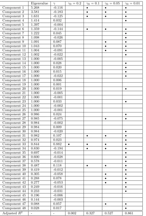
The model hasp48 input settings,X, that influence the behavior of technology markets and greenhouse owners. After running 100 simulations, we scale the columns of X and perform PCA and regression as described above. Table 2.4.1 gives the principal components’ eigenvalues,γ coefficients from regression and indicates which components were retained using different levels of γ0.

As we decrease γ0, the number of principal components retained increases and

the fit of the regression model improves, up to a certain point. The chosen values of γ0 result in regression models consisting of 1, 8, 16 and 36 principal components

as covariates, respectively. The regression model based on 36 principal components shows significantly better fit than the other models, pointing to the necessity of multiple factors in explaining the complex function of this ABM.

Of the criteria considered in this analysis, a value of γ0 0.01 is the most

conservative in terms of deleting principal components. As a result, this value will result in the fewest number of inputs being identified as irrelevant. This indicates the importance of the value ofγ0 in this procedure, especially in model development when

identifying an input as irrelevant could result in its removal from the ABM. Based on the four values of γ0 used above, we can examine which of the original 48 inputs

were identified as relevant with respect to the total production of the greenhouse owners, using both the forward and backward strategies discussed earlier in section 2.4.1. A summary of the model inputs and their relevance is given in Table 2.4.1.

The forward identification and backward elimination methods for classification of the original inputs agree in 78.6% of cases. All but one input was identified as irrelevant for some criteria, while there were five inputs that were identified as irrelevant based on all criteria. Four of the five inputs identified as irrelevant with

(45)

Table 2.1: Eigenvalues and γ coefficients for the 48 principal components of the Greenhouse model and indications of the components retained for values of γ0.

Ad-justedR2 _{is given for the four regression models to measure goodness-of-fit (adjusted}

R2 _{for regression using all 48 principal components is 0.863).}

Eigenvalue γ γ00.2 γ00.1 γ00.05 γ00.01 Component 1 5.268 -0.116 Component 2 3.581 -0.183 Component 3 1.631 -0.125 Component 4 1.414 0.032 Component 5 1.397 -0.004 Component 6 1.359 -0.144 Component 7 1.222 0.045 Component 8 1.098 -0.026 Component 9 1.091 0.087 Component 10 1.043 0.070 Component 11 1.004 -0.091 Component 12 1.002 -0.022 Component 13 1.000 -0.005 Component 14 1.000 0.028 Component 15 1.000 0.020 Component 16 1.000 0.015 Component 17 1.000 -0.022 Component 18 1.000 0.006 Component 19 1.000 0.001 Component 20 1.000 0.019 Component 21 1.000 -0.005 Component 22 1.000 -0.001 Component 23 1.000 0.033 Component 24 1.000 -0.002 Component 25 1.000 -0.001 Component 26 0.986 0.024 Component 27 0.985 -0.075 Component 28 0.984 -0.002 Component 29 0.984 0.009 Component 30 0.984 -0.020 Component 31 0.982 0.107 Component 32 0.974 0.023 Component 33 0.844 0.882 Component 34 0.830 -0.194 Component 35 0.697 -0.014 Component 36 0.600 -0.028 Component 37 0.578 -0.011 Component 38 0.487 0.118 Component 39 0.419 -0.012 Component 40 0.305 -0.058 Component 41 0.288 0.078 Component 42 0.277 -0.053 Component 43 0.249 -0.016 Component 44 0.233 -0.031 Component 45 0.196 -0.006 Component 46 0.144 -0.003 Component 47 0.088 0.057 Component 48 0.028 0.017 AdjustedR2 _- _- _0.002 _0.327 _0.527 _0.861

(46)

respect to the total greenhouse production (InfluenceRangeMain, TechA CO2Max, TechC HumMin, TechC LightMin) directly affect the behavior of technology markets and not greenhouse owners. Although these rules were found to be irrelevant with respect to total greenhouse production, they are central to the development of the technology markets and would likely be identified as relevant with respect to an emergent behavior based on technology improvement.

2.5 Discussion

The statistical theory related to ABMs is currently developing. While some theory and approaches for traditional models can be applied to ABMs, there are many fea-tures which are unique to ABMs and which require further investigation. Model val-idation protocol, assessments of model equivalence and model complexity for ABMs require the consideration of the multiple levels of behavior within the model to make determinations on these topics.

Model selection is a topic that remains to be thoroughly explored for ABMs. Elements from model selection for traditional statistical models such as predictive accuracy and error minimization can be incorporated into a model selection pro-cedure for ABMs, but often the lack of observed data and non-linearity of model behavior can limit the utility of such techniques (as discussed in chapter 3). While some of the theory on model complexity and model equivalence presented earlier in this chapter can be incorporated into a model selection protocol, more attention should be given to important elements in such a procedure.

(47)

Table 2.2: Original inputs which were identified as relevant with respect to total greenhouse production using forward identification (F) and backward elimination (B) methods, for values of γ0 p0.2,0.1,0.05,0.1q. Bullets () indicate variables

identifed as relevant and dashes (-) indicate irrelevant variables. A description of the inputs can be found in Kasmire et al. (2013).

γ00.2 γ00.1 γ00.05 γ00.01 Variable F B F B F B F B StubbornnessFactor - - - -InitialBankaccount - - - -CostPriceCooperativeMultiplicator - - - InfluenceRangeSec - - - -InfluenceRangeMain - - - -CostPriceRange - - - - - CostPriceMin - - - CostpriceMax - - - - - EnergyUseMin - - - EnergyUseMax - - - - -LifespanMin - - - LifespanMax - - - - - ImproveSameTechCounter - - - - - TechA TempMin - - - - - TechA CO2Max - - - -TechA HumMin - - - TechA LightMax - - - -TechB TempMax - - - TechB CO2Min - - - -TechB HumMin - - - TechB LightMin - - - -TechC TempMax - - - TechC CO2Max - - - TechC HumMin - - - -TechC LightMin - - - -TechD TempMax - - - -TechD CO2Max - - - -TechD HumMin - - - -TechD LightMin - - - VeggiesIdealTemp VeggiesIdealCO2 - - - - VeggiesIdealHum - - - - - VeggiesIdealLight - - - VeggiesPotentialGrowth - - - - - FlowersIdealTemp - - - FlowersIdealCO2 - - - - FlowersIdealHum - - - FlowersIdealLight - - - - - FlowersPotentialGrowth - - - ExternalTemp - - ExternalCO2 - - - - ExternalHum - - - - ExternalLight - - - FuelPrice - - VeggiesMarketPrice - - - FlowersMarketPrice - - - - VeggiesPurchasePrice - - - - - FlowersPurchasePrice - - - -

(48)

3

Gaussian Process Emulators

3.1 Overview

ABMs are often used to simulate complex real world processes. Running these sim-ulations is, in most cases, computationally taxing and cannot be carried out on the scale which we would like. Even in cases where the runtime is not a limiting issue for the ABM, generating thousands of runs is not an efficient method for perform-ing inference on the system beperform-ing modeled. To address this problem, we are able to utilize emulators. An emulator is a stochastic process that serves as a represen-tation of a simulator (in this case our ABM), which incorporates full probabilistic specification based on beliefs and knowledge. Using an emulator to serve as a sur-rogate for an ABM can be particularly useful in instances when the original model has a run time of several hours, and there is a need for simulations to run in real time. Such approaches have been investigated in the context of weather and envi-ronmental modelling (Margvelashvili, 2011) as well as transportation (Rasouli and Timmermans, 2013). Emulation in a Bayesian framework has been discussed in de-tail, notably in Kennedy and O’Hagan (2001), Craig et al. (2001), Bliznyuk et al. (2008) and Liu and West (2009).

(49)

3.2 Emulation of high-dimensional computer output

Some of the most prominent work in the utilization of emulators to model simulation output are Kennedy and O’Hagan (2000) and Kennedy and O’Hagan (2001). Here, I present an expansion on this methodology presented by Higdon et al. (2008) (dis-cussed in an earlier application in Higdon et al. (2004)), incorporating approaches developed by Santner et al. (2003).

Often, when the objective of an experiment is to understand and predict the behavior of complex systems and procedures, the subject of interest cannot be ob-served frequently enough to gather sufficient data to perform analyses. It is, however, possible to make use of computer models such as ABMs to simulate the process of interest. Naturally, some uncertainty will arise in the selection of certain inputs and parameters in our simulator, but this can be mitigated by utilizing actual observed data to guide the simulator and assist in performing inference.

To begin, suppose we have obtained nobservations of the system of interest. For

i1, ..., n, let the vectorxi represent the conditions under which theith ovservation of the system is made and define its dimension to be px. Let ypxiqdenote the actual

ith observation. (Note that the term ‘conditions’ will be problem-specific: In Higdon et al.’s study of implosion study, conditions specified the mass of the explosive used). The dimension of xi can vary depending on the system and experiment. Then, we have a simple model:

ypxiq ξpxiq pxiq (3.1) where ξpxiq is the response of the system under conditions xi and pxiq represents observation error. In many instances, systems will be well-enough understood that the errors can be treated as having a known distribution.

The ABM (simulator) will have certain calibration settingstwhich serve as inputs and affect the output. For ABMs, these calibrations will likely include, among other

(50)

things, the rules which determine agent behavior. While our goal is to model system behavior and observations, the values of the calibration settings are not known for our n actual observations. In this case, θ is used to represent the optimal, but unknown, values of these settings.

Letting ηpx,tq represent the ABM output under conditions x and calibration values t, the observed data y pypx1q, ..., ypxnqqT can now be modeled statistically:

ypxiq ηpxi,θq δpxiq pxiq (3.2) whereδpxiq is a stochastic term to account for systematic discrepancies between the ABM ηpxi,θq and the physical process ypxiq. This additive decomposition is based on Kennedy and O’Hagan (2001).

Again, because in many applications an ABM will be complex and computation-ally demanding, only a limited number of simulations can be obtained. Suppose we carry outmABM runs with conditions and calibration settingsx_j,t_j, producing out-put η pηpx₁,t₂, ..., ηpx_m,tmqqT_{. The ABM output can then be used as additional} data in setting up our emulator for analysis. Because of the complexity of the ABM, the function representing its output,η, is unknown. To address this uncertainty, we model η probabilistically in order to approximate ABM outputs for untried input values px,tq. Following O’Hagan (1978), Higdon et al. utilize a Gaussian Process model for ηpx,tq.

As a prior for ηpx,tqHigdon et al. proposed a Gaussian Process with a constant mean functionµpx,tqand a product covariance with power exponential form follwing Sacks et al. (1989). Recall from above that px dimpxq and define pt dimptq to be the dimension of the calibration settings. Thus, the covariance function will have