Harth, N. and Anagnostopoulos, C. (2018) Quality-aware Aggregation &
Predictive Analytics at the Edge. In: IEEE Big Data 2017, Boston, MA,
USA, 11-14 Dec 2017, pp. 17-26. ISBN
9781538627150 (doi:10.1109/BigData.2017.8257907)
This is the author’s final accepted version.
There may be differences between this version and the published version.
You are advised to consult the publisher’s version if you wish to cite from
it.
http://eprints.gla.ac.uk/149980/
Deposited on: 17 October 2017
Enlighten – Research publications by members of the University of Glasgow
Quality-aware Aggregation & Predictive Analytics at the Edge
Natascha Harth
School of Computing Science, University of Glasgow [email protected]
Christos Anagnostopoulos
School of Computing Science, University of Glasgow [email protected]
Abstract—We investigate the quality of aggregation and predictive analytics in edge computing environments. Edge analytics require pushing processing and inference to the edge of a network of sensing & actuator nodes, which enables huge amount of contextual data to be processed in real time that would be prohibitively complex and costly to transfer on centralized locations. We propose a quality-aware, time-optimized edge analytics model that supports communication efficient predictive modeling within the edge network. Our idea rests on the capability of edge nodes to intelligently decide when and which data to deliver and process in light of minimizing the communication overhead and maximizing the quality of analytics results. We provide mathematical modeling, performance and comparative assessment over real datasets showing its benefits in edge computing environments.
Keywords-Edge predictive analytics, quality of analytics, communication efficiency, optimal stopping theory.
I. INTRODUCTION
Focusing on the increase of sensing & computing devices in Internet of Things (IoT) environments, delivering data continuously towards centralized locations e.g., Cloud, is constrained by bandwidth, energy, computational power and data storage. Aggregation & predictive analytics at the edge of an (IoT) network is an emerging area [1] trying to overcome these constrains by analyzing data close to the sources. Analytics at the edge over dynamic data isdifferent from big data analytics over data at rest. It means carrying out the same kind of analysis, but moving more of it to the edge of the network, e.g., a car, an agricultural equipment in the field, or any other industrial device and exploiting only the local available resources. Pushing as much computing workload for analytics (e.g., regression/predictive models, outliers/concept drift detection), as close to the edge as possible brings serious benefits, particularly where commu-nication costs are high or where instant action/decision is needed. But, today’s edge capabilities are still relatively unsophisticated in light of quality of analytics, lacking anything like the computing power Cloud can provide.
We rest at the fact that pushing analytics towards the edge is feasible because of the increase of computational power on sensing & actuator devices. Their capabilities enables them to reduce network traffic and latency by supporting in-network real-time data analytics. However, analytics over contextual data at the edge should be imperatively pro-vided with high quality of outcomes, e.g., low prediction
errors, avoiding false alarms, taking into account efficient communication due to the above-mentioned constrains [1]. Within an edge network, it is deemed appropriate to intro-duce a methodology for providing quality aggregation and predictive analytics tasks departing from the traditional in-network data processing/delivery methods by exploiting the computing capability of the edge nodes.
Motivation: Let us consider the following motivating
scenario that demands high quality analytics & efficient communication at the edge for car driver mirco-sleep identi-fication [2]. In-car and driver mood-fatigue detection sensors locally sense the surrounding environment of the vehicle, road, and driver’s physiological, facial and driving behavior [2] and transmit data via 5G towards the Cloud for process-ing/classification and alert the driver/emergency services if irregular patterns are detected. We identify three cases: (a) the driver fell into a micro-sleep and the system identifies that; (b) the driver is awake while the system identifies a micro-sleep pattern; (c) the driver is awake and the system identifies that. Case (a) demands low latency and real-time reaction to prevent accidents with high certainty on the analytics outcome; using unreliable broadband for data transmission cannot support real-time identification leading to horrible consequences. Case (b) encounters a false alarm, e.g., due to missing or obsolete transmitting values, resulting in bad consequences, e.g., the driver got shocked by the risen alarm causing the car go off the road. In case (c) the car sensors continuously transmit data without any action occurrence, thus, resulting in humongous redundant values and unnecessary bandwidth consumption increasing latency. From such cases, it is challenging to support sophisticated decisions onwhenandwhichdata to process and deliver for supporting high quality of real-time analytics at the edge taking into account the induced communication overhead and latency. The research challenges this paper focuses on are: (1) deciding which data to communicate at the edge network withoutloosing quality of data and analytics outcomes at destination; (2) deciding whento deliver data in light of obtaining high quality of analytics; (3) reducing unnecessary communication between/among edge devices and/or Cloud for saving bandwidth and decreasing latency.
A. Related Work & Contribution
Many baseline approaches [3] (and the references therein) collectall data from IoT environments, e.g., Wireless Sen-sor Networks (WNS) to centralized locations for centrally performing analytics tasks requiring, thus, all devices to continuously sensing and communicating. However, due to bandwidth, latency and energy constrains alternative methodologies have been studied [4], [5], [6] especially for WSNs based on selective forwarding. In these approaches data are conditionally transmitted to central locations re-ducing communication overhead. However, such approaches focus only on communication efficiency and are unaware of the analytics tasks performed at the destination, thus, cannot be adopted to support high quality of analytics. Advanced selective forwarding methods [7], [8] deal with dynamic optimal decisions of finding the best time to deliver data in light of communication efficiency and reconstruction error minimization at the destination. Nonetheless, such optimal decision making is limited on communication overhead, not applied on the network edge and not taking into account its impact on the quality of advanced analytics like aggregation and predictive tasks. From the edge-analytics perspective, recent works [9], [10], [11] exploit the computational power of devices to launch (lightweight) algorithms directly at the data sources. However, such approaches are unaware of com-munication efficiency in the edge network as supported by the above-mentioned selective forwarding approaches. Our previous work [12] investigates the impact of a prediction-based selective forwarding decision, purely from the com-munication objective, on aggregation and predictive ana-lytics. This signals the necessity of introducing a hybrid and sophisticated decision making model onwhen&which data to process and deliver for trading between quality of (advanced) analytics and communication efficiency at the network edge. Our proposed method in this paper advances on time-optimized data forwarding and data processing decisions based on the historical patterns of data forwarding decisions and the predictive capability of the edge nodes to determine thebest timeand themost appropriatedata to deliver in light of maximizing the quality of aggregation and predictive analytics tasks at the destination being, in parallel, communication efficient. This is achieved based on a quality-aware, intelligent monitoring scheme over the cumulative reconstruction error at the destination under the principles of the Optimal Stopping Theory (OST) [13]. Ourcontribution is summarized as follows:
• an optimal, quality-aware decision making model deter-mining when and which data to deliver in the network edge in light of maximizing the quality of analytics by being communication efficient;
• mathematical analysis based on the principles of the
theory of optimal stopping [13] and incremental meth-ods for evaluating the optimal decision in real-time;
• two real-time model variants exploiting the compu-tational capabilities of the collaborating edge devices over real contextual data streams;
• comparative & performance assessment with aggre-gation and linear regression models using statistical & information theoretic metrics comparing our model with the methodologies [12], [4], [5], [6] following the selective forwarding scheme;
The paper is organized as follows: Section II discusses the rationale and provides fundamental definitions for the quality analytics metrics, while Section III presents the overall approach and problem formulation. Section IV elaborates on the solution fundamentals, while Section V reports on the performance and comparative assessment. Finally, Section VI concludes the paper with future research directions.
II. RATIONALE& FUNDAMENTALS A. Rationale
We abstract an edge network architecture through Edge Nodes (ENs) forming a layer between Sensing & Actuator Nodes (SANs) and the Cloud. Several SAN are connected to each EN, e.g., cloudlet, sink node in a WSN. Since ENs are located close to the SANs, contextual data should be efficiently transferred to them in real-time. The fundamental desiderata to materialize analytics at the edge are: (D1) the autonomous nature of SANs to locally perform sensing and determine whether and which data to transfer to ENs or not in light of minimizing the required communica-tion (overhead) at the expense of accurate and quality analytics tasks performed on ENs; (D2) the capability of ENs to locally reconstruct undelivered data and perform aggregation/predictive analytics tasks. We assume a tree-like topology in which a SAN i is connected with its EN j. We notate the neighborhood of EN j as the set of SANs
Nj ={1, . . . , nj}, i.e., i∈ Nj. We assume a discrete time
domain t ∈ T = {1,2, . . .} such that SAN i, at every
time instance t ∈ T, senses a d-dimensional row vector
xt = [x1t, . . . , xdt] ∈ Rd of contextual parameters, e.g.,
temperature, humidity, air pollutant chemical compounds. Hereinafter, we refer to xt∈Rd as context vectorat time t
which forms the communication between SAN iand ENj. A sliding windowWis specified by a fixed-size temporal extent N > 0 by appending new context vectors and discarding older ones on the basis of their appearance. At time t ∈ T, a sliding window W is a sequence of
all context vectors observed from t −N to t− 1, i.e.,
W = (xt−N,xt−N+1, . . . ,xt−1) and is most widely used
in continuous analytics [14], [15]. Aggregation analytics are evaluated over W, which change over time as the window slides. There are three categories of aggregation functions: distributive, algebraic and holistic [16]; notably MAX and
MIN are distributive,AVGis algebraic computed from SUM
andCOUNT, andQUANTILE,MEDIANare holistic. For in-stance,AVGis defined overW as:h(W) = N1 Ptk=t−Nxk.
One the most used predictive analytics models is the mul-tivariate linear regression [17]. Given a W with vectors
xt = [xint , youtt ] ∈ Rd representing input-output pairs
within the lastN measurements, the linear regression model estimates the current coefficientw ∈Rd, which interprets
the current dependency ofxin withyout:
w= arg min w0∈Rd 1 N N X t=1 ytout−(xint )>w0 2 (1) The predicted output yˆout provided by the actual linear
model w over W is yˆout = (xin)>w and the Root Mean
Square Error (RMSE) over npredictions is defined as:
= 1 n n X k=1 (youtk −yˆkout)2 !1/2 . (2)
The methodologies in [12], [4], [5], and [6] adopt a selec-tive forwarding rule to decide whether to deliver a context vector in the edge network or not in light of minimizing the communication overhead defying the quality of analytics tasks. Such methodologies are based on an Instantaneous Decision Making (IDM) using only (i) the current vector
xt and (ii) the expected (predicted) vector xˆt. To apply
this methodology in our context, SAN iis equipped with a vector prediction algorithmfi(xt−1, . . . ,xt−N), which uses
the recent pastN ≥1 sensed vectors stored in windowW
of sizeN to predict the future vectorxˆt at timet: ˆ
xt=fi(xt−1, . . . ,xt−N) =fi(W). (3)
SANiafter sensing xt predictsxˆt with prediction error:
et=d−
1
2kxt−xˆtk, (4)
wherekxk= (Pdk=1x2
k)1/2is the Euclidean norm ofxand
d−1/2 is a normalization factor to ensure that e
t ∈ [0,1],
given that x ∈ [0,1]d is scaled in the d-dimensional unit cube; each dimensionxk, k= 1, . . . , dranges in[0,1]. Such
prediction capability yields SAN able to decide whether to send x to its EN or not for processing based on aθ-based IDM rule:
• Case I If predicted xˆt differs from actual xt w.r.t.
decision thresholdθ∈(0,1), i.e.,et> θ, SANisends
xt to ENj.
• Case II Otherwise, i.e., et ≤θ, SAN idoes not send
xt to ENj and ENj is responsible for reconstructing
the undelivered vector locally.
In Case I, ENj receives the actualxtfrom SANi. In Case
II, ENj should adopt a reconstruction function ˜
xt=gj(ut−1, . . . ,ut−M) =gj(W), (5)
of the recent M ≥ 1 vectors u from its window W = (ut−M, . . . ,ut−1)to reconstruct the undeliveredxt, notated
byx˜tusing only historical vectors. The vectorsuin the EN’s
W correspond to either the actual x from SANi (Case I)
or the past locally re-constructed vectors x˜ from gj (Case
II):ut=xtifet> θ(Case I); otherwiseut= ˜xt=gj(W)
(Case II). The reconstruction error at ENj is then: at=
0 Case I,
kxt−x˜tk Case II.
(6) The aggregation & regression analytics functions are running on ENjfor eachsliding windowWcontainingM received and/or re-constructed vectors from the SANsi∈ Nj
depend-ing on cases I and II. We now introduce thediscrepancies of the analyticson EN due to the fact that EN does not always receive the actual vectors from SAN.
B. Definitions
Definition 1(Aggregation Analytics Discrepancy). Given a
pair (SANi, ENj), the aggregation discrepancyγ between the analytics output on EN j derived from aggregation function h over its window W and the actual analytics output on SANiover windowW∗, which contains the actual
context vectors (ground truth) is:γ=kh(W)−h(W∗)k.
The discrepancy γ denotes how much the aggregation results over W with vectors u on EN j differ from the aggregation results over W∗ with actual vectors x, should
SAN i have sent them all to EN j. In Case I we obtain γ = 0, while in Case II, γ ≥ 0 since EN j needs to re-construct undelivered vectors. We require to tolerate a low γin light of communication efficiency.
Definition 2(Regression Performance Discrepancy). Given
a pair (SANi, ENj), the regression discrepancyδis defined as the difference of the RMSE derived from the linear modelw estimated over ENj’s window W and the RMSE ∗derived from the ground truth linear modelw∗ estimated over the actual SANi’s vectors in W∗:δ=|−∗|.
Definition 3 (Model Fitting Discrepancy). Given a pair
(SANi, ENj), the model fitting discrepancyδ0is defined as the distance δ0 =kw−w∗k from the model w estimated over EN j’s window W and the ground truth model w∗
estimated over the actual SANi’s vectors inW∗.
The δ discrepancy measures the difference in the quality of the predictive performance of the predictive analytics (linear regression analytics) performed at ENj. The RMSE ∗ refers to the prediction w.r.t. w∗ over the actual pairs (xin, yout). Since ENj may not receive all the actual pairs
due to Case II, the derived model w results to a RMSE 6=∗.
The δ0 discrepancy measures the distance of the derived
linear model at ENj from the ground truth model at SAN i. Due to Case II, the model fitting achieved in ENj might be different (coefficients-wise) from the ground truth linear model fitting. We require to tolerate a low δ in terms of prediction performance and a lowδ0in terms of linear model fitting by being communication-efficient.
C. Problem Fundamentals
IDM attempts to increase the communication efficiency by saving significant network bandwidth but at the expense at analytics discrepancies. Fundamentally, IDM disregards the history of analytics discrepancies that ENs are experiencing. The vector forwarding decision is purely based on the current prediction error on SANs and does not take into consideration the past predictions. Obviously, the analytics discrepancies are unknown to EN since not all the actual vectors are sent for communication efficiency. On the other hand, such discrepancies are unknown to the SANs because, even if the actual vectors are sensed locally, SANs are not equipped with reconstruction and analytics functions. The only information a SAN has is a series of its prediction errors {et}. We will show that based on this series our
approach provides high quality of analytics while being communication efficient.
There are two major concerns in IDM:(C1) If θ is relatively high, SAN i scarcely updates EN j with actual vectors. Hence, ENj loses significant information, which is expected degrading analytics results. We encounter the same situation if the prediction erroretis relatively small; if for a
lowθ we encounteretθ, ENj does not follow the data
stream. This is happening e.g., when the predictorfiof SAN
iis very accurate. This is counterintuitive, since we desire to have an accurate predictorfi, but its instantaneous outcome
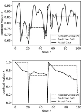
for decision making leads to the situation of information loss on ENj. Figure 1 (upper) shows the case wherefipredictor
(here, exponential smoothing) at SANiproduces predictions close to the actual data, thus, resulting in no communication and thus information loss at EN j, which re-constructs the data withgj(adopting exponential smoothing). (C2) If there
are certain outliers or novel cases/significant events in SAN i, SAN i delivers the associated vectors to ENj and then transits back to the state of non delivering vectors to ENj. In this situation, ENj accumulates most of the time outliers and novel vectors and, again, the re-constructed data do not follow the in-between actual data; see Figure 1 (lower).
Departing from IDM, given a decision thresholdθ∈(0,1) at SAN i, we will derive sufficient conditions for a novel, time-optimized, analytics discrepancy-aware decision mak-ing, where the vector forwarding decision is a function of both the desired error bound and correlation among data. When θ is very tight or the correlation is not significant, SAN i always has to forward its vectors to EN j. Due to the characteristics and inherent dynamics of SANs’ data, e.g., underlying data distribution evolves over time, predic-tion techniques may not work efficiently for a set of less predictable data. Moreover, there might be dependencies among data from neighboring SANs (data locality in Nj),
thus, EN j is capable of learning those dependencies in a communication-efficient way, as will be shown later.
0 20 40 60 80 100
time t
0.65 0.70 0.75 0.80 0.85 0.90 0.95co
nte
xt
va
lue
x
Reconstruction EN Prediction SAN Actual Data 0 20 40 60 80 100time t
0.0 0.2 0.4 0.6 0.8 1.0co
nte
xt
va
lue
x
Reconstruction EN Prediction SAN Actual DataFigure 1: The actual data sensed at SAN, the predicted data at SAN and the reconstructed data at EN vs. time demonstrating (upper) concern C1 and (lower) concern C2.
III. QUALITYANALYTICS-AWAREDECISIONMAKING A. Overall Approach
As IDM is not capturing the variability of the data stream inside EN, it results in information loss of the actual SAN’s data. Our approach departs from IDM, at the first instance, by taking into consideration past IDM decisions, i.e., decisions purely based on either et > θ or et ≤ θ.
Our approach elaborates on historical prediction error-aware decision making, which takes into consideration IDM deci-sions made at past time instances τ < t and the current decision at time t to decide on vector forwarding. Our method quantifies this historical context by accumulating the prediction errors eτ : τ ≤t with eτ ≤θ from which
forward decisions were taken. We encounter the past non-forward decisions as useful information in our method since this cumulative error on SAN i relates to the cumulative reconstruction error on ENj, thus, influencing the quality of analytics, as proved later. The non-forward decision indicates that the error is tolerable w.r.t. θ, however, its cumulation before a forward decision results to information loss, thus, cumulation of reconstruction error on the EN. Our idea is to exploit even those relatively small discrepancies for decision making and to tolerate up to a certain extent this cumulation. Nonetheless, in IDM, it is not instantly obvious the impact of the error cumulation on the quality of analytics at EN. We enforce SANinot only to track the
current prediction error at t but also the cumulative error up to t. Obviously, SAN i cannot monitor the expected reconstruction error at EN j to take a decision at t; recall that only the expected prediction error (up tot) is available to SANi. Based only on this information, the challenge is to monitor the behavior of the cumulative prediction error at SAN investigating which is its relation with the expected reconstruction error at EN, and up to which discrepancy tolerance this cumulative error is allowed to be in order to forward vectors from SAN i to EN j. We show that by monitoring the expected prediction error at SANi suffices to take more sophisticated and certain decisions on vector forwarding/non-forwarding.
Consider the case SAN i decides not to forward xt
to EN j and let us define ˆxt = ˜xt +ρt, where ρt is
the vector discrepancy of the predicted vector at SAN i and the reconstructed vector at EN j, given that et ≤ θ
and E[kρk] < ∞. Our target is to relate the conditional
expectation of the prediction error E[e|e ≤ θ] with the
expected reconstruction error E[a] given that SAN i does
not forward context vectors to ENj. We obtain that:
E[a] = E[kx−˜xk|e≤θ]P(e≤θ) + 0·P(e > θ)
= E[k(x−xˆ) + (ˆx−x˜)k|e≤θ]P(e≤θ)
≤ E[kx−ˆxk|e≤θ]P(e≤θ) +E[kρk
e≤θ]P(e≤θ)
≤ (E[e|e≤θ] +E[kρke≤θ])P(e≤θ) (7)
We obtain from (7) that the expected reconstruction error is bounded at least by the conditional expectation of the prediction error given that SANi does not forward vectors to EN, which is known at SAN i and the conditional expectation of the discrepancy E[kρke ≤ θ] derived by
the intrinsic difference of the reconstructed and predicted vectors. Interestingly, if SAN and EN adopt the same al-gorithm for prediction and reconstruction, e.g., exponential smoothing, then ρ can be directly known to SAN. Based on this outcome, our idea is that SAN tracks the cumulative sum of prediction errors for decision making as this reflects the cumulative reconstruction error shown in (7).
Consider now the event {et > θ} where SAN forwards
xt to EN thus there is on reconstruction error. Our method
takes also into account this decision to deal with a more sophisticated decision making since et> θ might not only
reflect the capability of the prediction algorithm but also the fact that the sensed data on SAN is rather unpredictable with significant peaks or outliers or even events that are of high importance. This knowledge cannot be derived instantly adopting IDM. Instead, a continuous (not necessarily strictly sequential) observations of events {et > θ} is deemed
appropriate to be taken into consideration for decision mak-ing. Our method proceeds with the quantification of these significant events by cumulating the scaled lower bound of the error excess w.r.t. θ, i.e., through a cumulative sum of quantities λθ for each event {et > θ} with λ > 0. As it
will be shown, the value of λ and the priority of vector forwarding upon the event{et> θ}leads to two variants.
Our method attempts to smooth the re-constructed data stream on the EN by taking into consideration (i) the cumulative prediction error avoiding concern C1 and (ii) the cumulation of events avoiding concern C2. This is achieved by optimally deciding on vector forwarding combining the error cumulation in cases {et ≤ θ} and the significance
of events in cases {et > θ}. This leads to a model which
drastically departs from IDM methods attempting to deal with the concerns C1 & C2.
B. Real-Time Decision Making Model
Our model optimally postpones vector forwarding in light of reducing communication and on the other hand increasing the quality of analytics. The problem is to identify when SAN should take a forward decision at t based on the current et, the cumulation of prediction errors and events
occurrences up to t. Given a fixed θ, which is application specific, if SAN delays to forward vectors to EN, we gain communication efficiency but EN cannot re-construct the data, thus, degrading the quality of analytics. If SAN forwards data with a high rate, we achieve high quality analytics at the expense of communication overhead. We seek a stochastic decision making model to deal with this trade-off by maximizing the delay tolerance (thus saving communication) at the expense of quality of analytics. Based on the conditional expectation of the prediction error at SAN, which is an upper bound of the expected reconstruc-tion error on EN (see (7)), we define the stochastic indicator Ztwhose value depends onet=kxt−xˆtk:
Zt=
λθ ifet> θ,
et ifet≤θ.
(8) A valueZt=λθindicates an event which cannot be
accu-rately predicted byfi at SAN w.r.t.θor signals a significant
peak or outlier/novelty att. A value Zt=et≤θ indicates
the acceptable error in term of quality tolerance, which is accumulated also at EN. In both cases, the cumulation of Zt values at t = 0,1, . . . enforces SAN to decide on
vector forwarding based on the history of {et ≤ θ} and
{et> θ}. We abstract this cumulative enforcement through
the cumulative sum of either prediction errors or tolerances up to t, i.e., St =
Pt
τ=0Zτ. Since the quantity St up to
tprovides information to SAN whether to further postpone vector forwarding or not, we define the reward tolerance functionat timetas:
Yt=βtSt=βt t X
τ=0
Zτ, (9)
with tolerance discount factor β ∈ (0,1) acting as an adviser on delaying vector forwarding or not.Ytrepresents
the stochastic tolerance for non-forward decisions up to t. The idea is to postpone vector forwarding as much as
possible, thus saving communication, but not to degrade the analytics quality at EN. β → 1 suggests SAN to further postpone vector forwarding in light of minimizing the communication, whileβ→0suggests SAN to proceed with vector forwarding at an earlier stage in light of minimizing the reconstruction error at EN. Based on the randomness of the events (randomness of Zt and St), SAN tries to
find theoptimal vector forwarding timet∗ to maximize the expectation of Yt,E[Yt], given fixedβ andθ. Formally:
Problem 1. Find the optimal vector forwarding timet∗ at
which the supremum of the expectation ofYtis attained: sup
t≥0E
[Yt]. (10)
SAN tracks the Zt values at t= 0,1. . ., and decides to
forward xt at time t∗, which maximizes E[Yt]. Based on
the value of λ∈ {0,1} we contribute with two variants of our method to cope with both C1 and C2 and provide the trade-off between quality analytics and communication.
IV. QUALITY-AWAREOPTIMALVECTORFORWARDING A. Solution Fundamentals
We first prove that the optimal forwarding time t∗ for Problem 1 exists provided in Theorem 1 based on the principles of OST [13] and provide an optimal forwarding rule for evaluating it at Theorem 2. Then, we report on the two proposed variants.
Theorem 1. The optimal vector forwarding time for
Prob-lem 1 exists.
Proof:Based on the principles of OST [13], to prove the existence oft∗ we need to prove that the conditions A1 and A2 for Yt in (9) are satisfied: (A1)lim suptYt≤Y∞ = 0
almost surely and (A2) E[suptYt] < ∞. A1 implies that
with the elapse of time (t → ∞) the reward should go to zero, i.e., Y∞ = 0, since no vector delivery with indefinite
horizon is useless due to extremely high reconstruction error at EN; Y∞ = 0 represents the reward of an endless non
delivery phase. A2 implies that the expected reward under any policy is finite. We first focus on the supremum limit of Ytnotated bylim suptYt, i.e., the limit ofsuptYtast→ ∞
orlimt→∞(sup{Yk :k≥t}). Note,Ztare non-negative and
from the strong law of numbers(1tPtk=1Zk)→E[Z]:
Yt=tβt(St/t) =tβt(1/t) t X
k=1
Zk∼tβtE[Z]a.s.→ 0,
that islimt→∞suptYt= 0. Moreover, we haveY∞= 0 by
definition, thus, A1 is satisfied. For A2, we have sup t Yt= sup t βt t X k=1 Zk ≤sup t t X k=1 βkZk≤ ∞ X k=1 βkZk. Hence, E[sup t Yt]≤ ∞ X k=1 βkE[Z] =E[Z] β 1−β <∞. Therefore, it is shown that the optimal forwarding time in (10) exists.
Theorem 2. SAN decides to forward vectorxt∗ at time t∗:
t∗ = inf{t≥1| t X k=1 Zk≥ β 1−βE[Z]}. (11)
Proof: Since Ytare non-negative, Problem 1 is
mono-tone[18] thus the optimal time t∗ is obtained by the one-stage look-ahead optimal rule(1-sla):
t∗= inf{t≥1|Yt≥E[Yt+1]}.
The adoption of 1-sla is optimal since suptYt has finite
expectation (equal toE[Z]1−ββ ) andlim suptYt= 0almost
surely as proved in Theorem 1. Hence, t∗ is estimated through the principle of optimality; suppose thatSt=sand
SAN decides that it is optimal to forward a vector. Then, the current reward ofβtsis at least as large as any expected
E[(1−ββ )
t+τ(s+S
τ)], which means that:s(1−E[(1−ββ ) τ])≥ E[(1−ββ )
τS
τ] for all times τ. This must hold true for all
s0≥s, thus, the optimal timet∗for somes0must be of the
formt∗= inf{t≥1|St≥s0}. That is, SAN forwards at the
firsttfor whichSt≥s0. Now, the tolerance for forwarding
s0, must be the same as the tolerance for continuing using
the 1-sla that forwards the first time the sum of tolerances is positive. That is,s0 must satisfy the equation
s0=E[( β
1−β)
τ(s
0+Sτ)],
withτ = inf{t≥1|Sτ >0}. SinceY is non-negative, we
obtain τ ≡ 1 and Sτ ≡ Y [18] and then replacing with
s0 = 1−ββ E[Y] we obtain: t∗ = inf{t ≥ 1|Ptk=1Zk ≥ β
1−βE[Z]}.
B. Evaluation of the Optimal Vector Forwarding Time Theorem 2 provides us with the optimal forwarding time t∗ for SAN. At each time t SAN observes the events
{et ≶ θ}, evaluates Zt andSt. If the criterion (11) holds
true then SAN forwards x to EN and resets the sum to zero starting a new ‘era’ of optimal vector forwarding. The triggering of (11) requires the knowledge ofE[Z] at SAN,
which is now associated with the conditional expectation of the prediction errorE[e|e≤θ]as discussed in Section III-A, which is known to SAN. We contribute with an incremental mechanism to estimateE[Z]based on the expected
predic-tion error on SAN. Specifically we obtain that
E[Z] = E[Z|e > θ]P(e > θ) +E[Z|e≤θ]P(e≤θ)(12)
= λθ−
Z θ
0
whereI(θ) =R0θ(λθ−e)p(e)deandp(e)is the Probability Density Function (PDF) of the prediction error in SAN. Notably, the criterion (11) is based on the estimation ofI(θ), which involves estimation of p(e). The approximation of p(e)att, notated bypˆ(t)(e), is based on incremental Kernel
Density Estimation (KDE) from the sequencee1, . . . , et:
ˆ p(t)(e) = 1 t t X k=1 Kh(e−ek), (13)
where Kh(u) is a kernel function, unimodal, symmetric,
non-negative that centers at zero and integrates to unity while the windowhcontrols the degree of smoothing of the estimation. The PDF ofeis then estimated incrementally as:
ˆ
p(t)(e) = t−1 t pˆ
(t−1)(e) +1
tKh(e−et) (14) withpˆ(1)(e) =Kh(e−e1). The integral I(θ)can be then
incrementally estimated based on pˆ(t−1)(e)andetatt >1
based on the recursion:
I(t)(θ) = t−1 t I (t−1)(θ) +1 t Z θ 0 (θ−u)Kh(u−et)du (15)
Whenetis obtained by SANonlythe evaluation ofq(t)(e) =
1
t Rθ
0(θ−u)Kh(u−e)duis needed for checking the criterion
(11) with initial I(1)(θ) = q(1)(e
1) at time t = 1. There
are certain kernels Kh that can be adopted here, e.g.,
Epanechnikov and Gaussian kernel. The Gaussian kernel is mostly used due to its convenient mathematical properties and, especially, when dealing with PDF estimation. We adopt the Gaussian Kh(u) = √21πhe−
1 2(uh)
2
where the optimal value of h is h∗ = 1.06 minˆσ,1.Rˆ34T−15 [19], where σˆ is the standard deviation ofe, Rˆ is the interquartile range, andT is the number of training error values. Based onKh∗,
SAN easily calculates q(t)(e
t)1 and evaluates the criterion
(11) for vector forwarding inO(1) throughI(θ)in (13). C. Quality-Aware Model Variants
We propose two variants depending on the value of λ, which plays a significant role on decision making. With λ = 1, we obtain the pure Optimal Vector Forwarding (OVF) variant, which usesθas the least tolerance value ifet
exceedsθin (8). OVFalwaysincreases the cumulative sum Steven if the predictorf in SAN produces accurate forecast
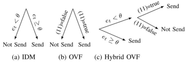
w.r.t.θor not. This presents astrictvariant which takes into consideration even the relatively small prediction errors for deciding on vector forwarding. Figure 2 (b) shows the OVF decision tree, which is purely based onStand a forwarding
decision is triggered w.r.t. (11) compared to IDM (Figure 2 (a)). With λ = 0, we obtain a variant which imposes a penalty only when the predictor f in SAN forecasts correctly the expected context and acts immediately when
1Due to space limitations, the formulate ofq(t)(e
t)withh∗is omitted. Not Send et < θ Send e t ≥ θ (a) IDM Not Send (11)=f alse Send (11)=true (b) OVF Send (11)=true Not Send (11)=f alse et< θ Send et≥ θ (c) Hybrid OVF
Figure 2: The decision trees for IDM and variants OVF and HOVF. OVF is triggered based on (11); HOFV combines both decision trees of IDM and OVF.
the prediction error exceeds θ. In this case, St does not
always monotonically increase thus making a forwarding decision based on the inherent prediction capability of SAN. This variant, called as Hybrid OVF (HOVF), combines both the pure OVF in the case where{et< θ}, thus, accumulating
only the tolerances due to the prediction capability of the SAN (coping with C1), and the IDM in the case where the current prediction error exceeds θ, thus, capturing immedi-atelyany significant event/outlier/novelty (coping with C2). Figure 2(c) shows the HOVF decision tree fusing decisions of OVF for C1 and IDM for C2.
Both variants require a vector prediction algorithm fi at
SAN i following the evolving nature of the data streams and a reconstruction algorithmgj at ENj that supports the
analytics tasks for the pair(i, j). We are seeking to reduce the computational power for prediction and reconstruction at SAN and EN thus using a small fraction of their computing power we adopt the multivariate exponential smoothing [20], used for time series forecast, as an ideal predictor with computational complexity O(d) in a d-dimensional space2. Exponential smoothing weighs the current vector with the historic vectors and is adopted as the function fi
for predicting ˆx and as the function gj for re-constructing ˜
x. At timet, a smoothed vectorstis calculated by using the
current vectorxt and the previous smoothed vectorst−1:
st=αxt+ (1−α)st−1, (16)
initializing withs0=x0 andα∈[0,1]. A higherαdenotes
more importance to the current vector and less importance to the historic vectors; normally,α= 0.7 [20]. The calculated smoothed vector st−1 = [s1,t−1, . . . , sd,t−1] refers to the
predicted vectorxˆt: xˆt =fi(W) =st−1 with the window
W= (st−1)at SANicontaining only the recent smoothed
vector. ENj, at timet either receivesxtor nothing. In the
former case ENjinserts the deliveredxtinto its windowW
(which is associated with SANi∈ Nj) discarding the oldest
vector, i.e., ut =xt. In the latter case EN j re-constructs
the undelivered vector with the available vectors u reside currently in itsW using exponential smoothing gj(W).
V. PERFORMANCE& COMPARATIVEASSESSMENT A. Experimental Setup & Analytics Quality Metrics
We compare the performance of the OVF and HOVF variants with the models in [12], [4], [5], and [6], which implement the IDM methodology, over real contextual data described in [21]. The dataset contains T = 104 context
vectors in a 12-dimensional (d = 12) real data space corresponding to sensing air quality parameters reflecting 12 SANs of an edge network connecting with EN. For ex-amining the reconstruction and aggregation analytics (exper-imenting with theAVG aggregation function, i.e., h(W)≡
AVG), all context vectors are normalised and scaled, i.e., each parameterx∈Ris mapped to x−µσ with mean valueµ
and varianceσ2and scaled in [0,1], thus vector x∈[0,1]d.
For examining the discrepancy in the regression analytics (in terms of performance and model fitting), after vector noram-lisation, we divided the 12 air quality sensors to four SANs, where in each SAN two sensors serve as thexin while the
remaining sensor serves as the responseyout; we added the
constant 1 to xinto allow intercept in the linear regression
model. The regression task at EN is therefore to predict the value of the 3rd sensor in each SAN using the first two. The discrepancy in the regression RMSE is achieved by 10-fold cross validation. The thresholdθ∈ {10−5, . . . ,0.3}ranging from sensitive to less sensitive quality of data capturing a range of context-aware applications, while the OVF (HOVF) factor β ranges in {0.1, . . . ,0.999} for investigating the impact of the forwarding tolerance on the quality of ana-lytics. For all SANs and the EN, the exponential smoother (predictor and re-constructor) adopts α= 0.7 as suggested in [20], while the window at each SAN is N = 1(due to exponential smoothing) and at EN,M = 10, for each SAN. Our target is to compare OVF (HOVF) with IDM vari-ants in terms of communication overhead, reconstruction error, quality of aggregation tasks, and quality of predic-tive analytics (regression performance and model fitting). We measure the percentage of communication, i.e., context vectors transmitted by each model for each pair (SANi, EN j) against the baseline solution, which forwards all actual vectors from SANs to EN. In terms of analytics quality, we examine the reconstruction error a due to undelivered vectors and the aggregation analytics outcome γ adopting the Symmetric Mean Absolute Percentage Error (SMAPE) per SAN. We use SMAPE as a quality metric due to its unbiased properties [22] representing a percentage value in [0,100]defined as: SMAPE = 100T PTt=1 at
kxtk+kx˜tk and
SMAPE= 100T PTt=1 γt
kh(W)k+kh(W∗)k. Moreover, we adopt
Kullback-Leibler (KL) divergence as a quality metric to measure the theinformation lossEN experienced due to the applied models over each reconstructed vector dimension ˜
xfrom the actual dimension xafter estimating their PDFs p(˜x)andp(x), respectively, defined by:KL(p(˜x)kp(x)) = R1
0 p(˜x) log
p(˜x)
p(x)dx.KL indicates the amount of information
lost when EN j approximates the actual vectors at SANs i due to undelivered vectors. For assessing the quality of predictive analytics, we measure the discrepancy δ in the linear prediction performance w.r.t. RMSE and the model fitting discrepancyδ0 in the actual and approximated linear models as defined in Section II-B.
B. Experimental Evaluation & Results
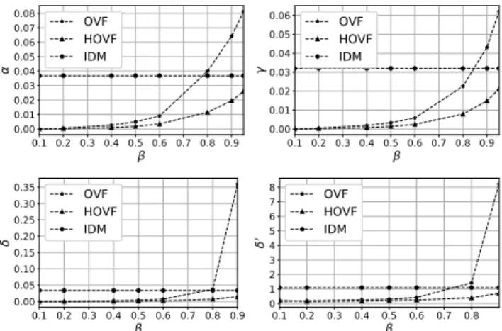
We identified during evaluation that the tolerance discount factor β is of high influence for the two optimal vector forwarding variants. In contrast, IDM does not depend onβ and only variates with changing the thresholdθ. Considering a fixedθvalue, which is application-specific, for all models OVF, HOVF and IDM, we examine the quality of analyt-ics at EN in terms of reconstruction error a, aggregation analytics γ, regression performance δ and model fitting δ0 discrepancies as the tolerance factorβ increases. As shown in Figure 3 increasing inβ results in increasinga,γ,δand δ0values for OVF and HOVF; IDM remains constant during all variations of β. A high β value refers to more tolerant OVF variants since they decide to further postpone vector forwarding in light of communication efficiency; however at the expense of quality of analytics. Specifically, OVF adopt-ing β >0.8 produces for all performance metrics a higher discrepancy than IDM. However, by adopting β ≤ 0.8, OVF benefits of lower analytics discrepancies compared to IDM reflecting its flexibility of being less tolerant in terms of analytics quality while being communication efficient w.r.t. IDM. The HOVF variant achieves a better trade-off between tolerance and communication efficiency than the OVF and IDM models considering both concerns C1 and C2 simultaneously. Specifically, HOVF obtains an asymptotic behavior towards IDM with increase of tolerance in light of being communication efficient in all metrics. Interestingly, the analytics discrepancies for HOVF are with all values of β below the IDM, indicates that HOVF is deemed an appropriate method to be adopted for high quality analytics tasks w.r.t. IDM and OVF given a fixedθ; similar results are obtained for otherθvalues, which are not presented here due to space limitations. Even OVF can be preferred over IDM havingβ≤0.8achieving higher quality analytics outcomes. Besides the consideration of the analytics discrepancy, we also have to evaluate the information loss at EN with increas-ing the tolerance factor β (to achieve less communication overhead) with respect to how the reconstructed data PDFs at EN diverge from the actual data PDFs at SANs due to optimal vector forwarding decisions. Figure 4 (upper-left) illustrates that with the raise of β, the information loss, measured by KL metric, increases, which means that EN is less able to approximate the undelivered actual vectors of SANs. By adopting the IDM model as an upper bound of KL divergence value to compare the OVF and HOVF variants against, we observe that HOVF does not exceed this value of the IDM model even if the tolerance factor
is high (β → 1). This denotes the capability of HOVF to optimally decide not only when to forward vectors to SAN but also which vectors helping SAN to accurately capture the statistical characteristics of the actual vectors at SANs. Similar behavior is achieved by OVF having β≥0.8; this differentiates HOVF from OVF in determining not only when but also which vector to deliver as reflected by the treatment of the concerns C1 and C2. Both optimal variants provide edge applications with the flexibility of achieving high quality of analytics, satisfiable capture of the statistical characteristics, and communication efficiency by tuning the tolerance factor β given a pre-determined application-specific accuracy thresholdθ.
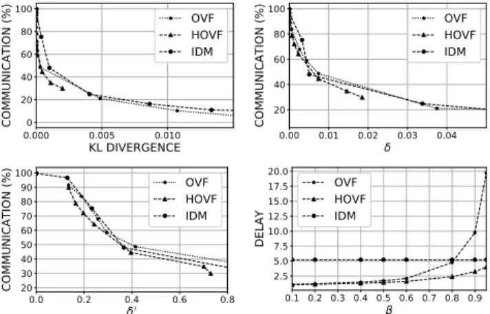
Figure 4 (upper-right) examines the induced (%) of com-munication for θ ∈ {0.01,0.06} for all models against the tolerance factor β. Obviously, as β → 1 both opti-mal forwarding models reduce the communication between SANs and EN, where IDM is not flexible to tune this percentage. It is interesting to mention that the HOVF variant exhibits an asymptotic behavior towards the IDM with an increase of β (for both θ values), thus, liaising this with its quality of analytics performance in Figures 3 and 4 (upper-left), demonstrates the successful trade-off between quality of analytics and communication efficiency. The HOFV variant provides us with the flexibility of obtaining high analytics quality while being communication efficient, which are the fundamental desiderata in edge analytics as discussed in Section II-A, while the OVF variant can support both desiderata having β ∈ (0.5,0.8). Figures 4 (lower-left/right) and 5 (upper-(lower-left/right) show the trade-off (%) of communication against reconstruction error a, aggregation discrepancyγ, KL and regression discrepancyδfor OVF and HOVF varyingβ from the lowest to highest withθ= 0.06; for IDM varyingθfrom the lowest to highest. Both variants outperform the efficiency of IDM. Therefore, by adopting HOVF not only decrease the communication overhead and provides less information loss on EN, but also guarantees better quality of analytics at EN. Finally, Figure 5 (lower-right) shows the expected intermediate time between two consecutive forwarding decisions, i.e., the expected delay for vector forwarding, for all models against β having θ= 0.06for IDM. HOVF assumes the lowest delay in vector forwarding, since it attempts to forward the most appropriate vectors for achieving high quality of analytics, as discussed above. Interestingly, asβ→1, the expected delay of HOVF approaches that of IDM indicating that even both models assume quite similar forwarding rates, HOVF intelligently choses to forward the best vectors for guaranteeing high an-alytics quality compared to the quality-unaware IDM. OVF appears more communication efficient especially for high β values at the expense of quality of analytics, while IDM remains inflexible in adapting to communication overhead constraints and accuracy of analytics results.
0.1 0.2 0.3 0.4 0.5 0.6 0.7 0.8 0.9 β 0.00 0.01 0.02 0.03 0.04 0.05 0.06 0.07 0.08 α OVF HOVF IDM 0.1 0.2 0.3 0.4 0.5 0.6 0.7 0.8 0.9 β 0.00 0.01 0.02 0.03 0.04 0.05 0.06 γ OVF HOVF IDM 0.1 0.2 0.3 0.4 0.5 0.6 0.7 0.8 0.9 β 0.00 0.05 0.10 0.15 0.20 0.25 0.30 0.35 δ OVF HOVF IDM 0.1 0.2 0.3 0.4 0.5 0.6 0.7 0.8 β 0 1 2 3 4 5 6 7 8 δ ′ OVF HOVF IDM
Figure 3: (Upper-left) reconstruction errora vs.β; (upper-right) aggregation discrepancy forAVGγvs.β; (lower-Left) regression discrepancy δ vs. β; (lower-right) model fitting discrepancyδ0 vs.β. Fixed thresholdθ= 0.06.
0.1 0.2 0.3 0.4 0.5 0.6 0.7 0.8 0.9 β 0.000 0.002 0.004 0.006 0.008 0.010 0.012 0.014 0.016 K L DI V ER G EN C E OVF HOVF IDM 0.1 0.2 0.3 0.4 0.5 0.6 0.7 0.8 0.9 β 20 40 60 80 100 C O M M U N IC A TI O N ( % ) OVF OVF(θ=0.1) HOVF HOVF(θ=0.1) IDM IDM(θ=0.1) 0.1 0.2 0.3 0.4 0.5 0.6 0.7 0.8 0.9 SMAPE for α (%) 20 30 40 50 60 70 80 90 100 C O M M U N IC A TI O N ( % ) OVF HOVF IDM 1 2 3 4 5 SMAPE for γ (%) 20 40 60 80 100 C O M M U N IC A TI O N ( % ) OVF HOVF IDM
Figure 4: (Upper-left) KL divergence vs. β (θ = 0.06); (upper-right) (%) communication vs.β for IDM, OVF and HOVF with θ = {0.01,0.06}; Trade-off for OVF, HOVF and IDM withθ = 0.06 and all β between (%) communi-cation and (lower-left) reconstruction errora, (lower-right) aggregation discrepancyγ.
VI. CONCLUSIONS& FUTUREWORK
We propose a novel, quality-aware and time-optimized decision making model for achieving high quality edge analytics while being communication efficient. We introduce the fundamental quality metrics and provide two variants exploiting the sensing & computational capabilities of nodes to perform on-line decision making. The edge nodes are enhanced to intelligently decide when and which data to deliver for guaranteeing high quality of data reconstruction, aggregation and linear regression analytics. We provide mathematical analyses based on the principles of optimal stopping theory, while evaluating and comparing the mod-els performance with other methodologies following the
0.000 0.005 0.010 KL DIVERGENCE 0 20 40 60 80 100 C O M M U N IC A TI O N ( % ) OVF HOVF IDM 0.00 0.01 0.02 0.03 0.04 δ 20 40 60 80 100 C O M M U N IC A TI O N ( % ) OVF HOVF IDM 0.0 0.2 0.4 0.6 0.8 δ′ 20 30 40 50 60 70 80 90 100 C O M M U N IC A TI O N ( % ) OVF HOVF IDM 0.1 0.2 0.3 0.4 0.5 0.6 0.7 0.8 0.9 β 2.5 5.0 7.5 10.0 12.5 15.0 17.5 20.0 DE LA Y OVF HOVF IDM
Figure 5: Trade-off for OVF, HOVF and IDM between (%) communication and left) KL divergence, (upper-right) regression discrepancyδ, (lower-left) model fittingδ0; (lower-right) expected delay vs. β (θ= 0.06).
instantaneous decision making paradigm. Our approach is deemed appropriate to edge analytics being flexible to cope with the trade-off quality & communication overhead. Our future research agenda includes leveraging edge analytics by pushing predictive modeling & analytics to sensing/actuator devices expecting limited data transmission.
ACKNOWLEDGEMENT
This research is funded by the EU H2020 GNFUV Pro-ject/Action RAWFIE-OC2-EXP-SCI, under the EC Future Internet Research Experimentation (FIRE+) initiative.
REFERENCES
[1] M. Satyanarayanan, P. Simoens, Y. Xiao, P. Pillai, Z. Chen, K. Ha, W. Hu, and B. Amos, “Edge analytics in the internet of things,” IEEE Pervasive Computing, vol. 14, no. 2, pp. 24–31, 2015.
[2] W. Tu, L. Wei, W. Hu, Z. Sheng, H. Nicanfar, X. Hu, E. C.-H. Ngai, and V. C. M. Leung.
[3] L. G. Rioset al., “Big data infrastructure for analyzing data generated by wireless sensor networks,” in IEEE Big Data Congress, 2014, pp. 816–823.
[4] A. Manjeshwar and D. P. Agrawal, “Teen: Arouting protocol for enhanced efficiency in wireless sensor networks,” in Proceedings of the 15th International Parallel & Distributed Processing Symposium. IEEE, 2001, p. 189.
[5] ——, “Apteen: A hybrid protocol for efficient routing and comprehensive information retrieval in wireless sensor net-works,” inIEEE IPDPS ’02, 2002, pp. 48–.
[6] H. Jiang, S. Jin, and C. Wang, “Prediction or not? an energy-efficient framework for clustering-based data collection in wireless sensor networks,” IEEE Trans. on Parallel and Distributed Systems, vol. 22, no. 6, pp. 1064–1071, 2011.
[7] N. Cheng, N. Lu, N. Zhang, T. Yang, X. S. Shen, and J. W. Mark, “Vehicle-assisted device-to-device data delivery for smart grid,” IEEE Trans. on Vehicular Technology, vol. 65, no. 4, pp. 2325–2340, 2016.
[8] C. Anagnostopoulos, “Time-optimized contextual information forwarding in mobile sensor networks,” J. Parallel and Dis-tributed Computing, vol. 74, no. 5, pp. 2317–2332, 2014. [9] G. Kamath, P. Agnihotri, M. Valero, K. Sarker, and W.-Z.
Song, “Pushing analytics to the edge,” inIEEE GLOBECOM, 2016, pp. 1–6.
[10] C. Anagnostopoulos, “Quality-optimized predictive analyt-ics,” Applied Intelligence, vol. 45, no. 4, pp. 1034–1046, 2016.
[11] M. Gabel, D. Keren, and A. Schuster, “Monitoring least squares models of distributed streams,” in21th ACM SIGKDD KDD, 2015, pp. 319–328.
[12] N. Harth, C. Anagnostopoulos, and D. Pezaros, “Predictive intelligence to the edge: Impact on edge analytics,”Evolving Systems, 2017.
[13] G. Peskir and A. Sirjaev,Optimal stopping and free-boundary problems. Birkhuser Basel, 2006.
[14] M. Dallachiesa, G. Jacques-Silva, B. Gedik, K.-L. Wu, and T. Palpanas, “Sliding windows over uncertain data streams,” KAIS, vol. 45, no. 1, pp. 159–190, 2015.
[15] K. Patroumpas and T. Sellis, “Maintaining consistent results of continuous queries under diverse window specifications,” Information Systems, vol. 36, no. 1, pp. 42–61, 2011. [16] J. Gray, S. Chaudhuri, A. Bosworth, A. Layman, D. Reichart,
M. Venkatrao, F. Pellow, and H. Pirahesh, “Data cube: A relational aggregation operator generalizing group-by, cross-tab, and sub-totals,” Data Mining & Knowledge Discovery, vol. 1, no. 1, pp. 29–53, 1997.
[17] M. Kuhn and K. Johnson, Applied predictive modeling.
Springer, 2013, vol. 26.
[18] H. Robbins, D. Sigmund, and Y. Chow, “Great expectations: the theory of optimal stopping,”Houghton-Nifflin, vol. 7, pp. 631–640, 1971.
[19] B. W. Silverman, Density estimation for statistics and data analysis. Chapman and Hall, London, 1986, vol. 26. [20] J. Durbin and S. J. Koopman, Time series analysis by state
space methods. OUP Oxford, 2012, vol. 38.
[21] S. De Vito, E. Massera, M. Piga, L. Martinotto, and G. Di Francia, “On field calibration of an electronic nose for benzene estimation in an urban pollution monitoring scenario,”Sensors and Actuators B: Chemical, vol. 129, no. 2, pp. 750–757, 2008.
[22] C. Tofallis, “A better measure of relative prediction accuracy for model selection and model estimation,” J. Operational Research Society, vol. 66, no. 8, pp. 1352–1362, 2015.