Fast Inference for Intractable Likelihood Problems
using Variational Bayes
David Gunawan
∗Minh-Ngoc Tran
†Robert Kohn
‡Abstract
Variational Bayes (VB) is a popular statistical method for Bayesian in-ference. The existing VB algorithms are restricted to cases where the likeli-hood is tractable, which precludes their use in many interesting models. Tran et al. (2015) extend the scope of application of VB to cases where the like-lihood is intractable but can be estimated unbiasedly, and name the method “Variational Bayes with Intractable Likelihood (VBIL)”. This paper presents a version of VBIL, named Variational Bayes with Intractable Log-Likelihood (VBILL), that is useful for cases, such as big data and big panel data models, where only unbiased estimators of thelog-likelihoodare available. In particular, we develop an estimation approach, based on subsampling and the MapReduce programming technique, for analysing massive datasets which cannot fit into a single desktop’s memory. The proposed method is theoretically justified in the sense that, apart from an extra Monte Carlo error which can be controlled, it is able to produce estimators as if the true log-likelihood or full data were used. The proposed methodology is robust in the sense that it works well when only highly variable estimates of the log-likelihood are available. The method is illustrated empirically using several simulated datasets and a big real dataset based on the arrival time status of U. S. airlines.
Keywords. Pseudo Marginal Metropolis-Hastings, Debiasing Approach, Big Data, Panel Data, Difference Estimator.
1
Introduction
Given an observed dataset y and a statistical model with a vector of unknown pa-rametersθ, a major aim of statistics is to carry out inference about θ, i.e., estimate the underlying θ that generated y and assess the associated uncertainty. The likeli-hood functionp(y|θ), which is the density of the datayconditional on the postulated model and the parameter vectorθ, is the cornerstone of many statistical procedures. Most of the popular likelihood-based methodologies, such as Maximum Likelihood Estimation, Markov chain Monte Carlo (MCMC), Importance Sampling and Vari-ational Bayes, require exact evaluations of the likelihood p(y|θ) at each value of θ.
∗School of Economics, UNSW Business School, [email protected]
†Business Analytics, University of Sydney Business School, [email protected] ‡School of Economics, UNSW Business School, [email protected]
In many modern statistical applications, however, the likelihood function is either analytically intractable or computationally intractable, which makes it difficult to use likelihood-based methodologies.
An important situation in which the log-likelihood is computationally intractable is Big Data (Wang et al., 2015), where the log-likelihood function, under the inde-pendence assumption, is a sum of a very large number of terms that is too expensive to compute. Large panel data models (Fitzmaurice et al., 2011) are another example where the log-likelihood is both analytically and computationally intractable as it is a sum of many terms, each of which is the log of an integral over the random effects and cannot be computed analytically.
There are several methods in the literature that work with an intractable like-lihood. A remarkable approach is the pseudo-marginal Metropolis-Hastings (PMMH) algorithm (Andrieu and Roberts, 2009), which replaces the likelihood in the Metropolis-Hastings ratio by its non-negative unbiased estimator and is able to generate sam-ples from the posterior. Like standard Metropolis-Hastings algorithms, PMMH is extremely flexible. However, this method is highly sensitive to the variance of the likelihood estimator, the chain might get stuck and mix poorly if the likelihood esti-mates are highly variable (Flury and Shephard, 2011). This is because the asymptotic variance of PMMH estimators increases exponentially with the variance of likelihood estimator (Pitt et al., 2012). The PMMH method can be computationally expensive and is not parallelizable, which makes it unsuitable for Big Data applications.
This paper develops fast and efficient methodologies for statistical inference based on VB, with a special focus on computational efficiency and challenging situations such as Big Data and in particular Big Panel Data - a mainstream area of research in statistics and its related fields in the next decade. The existing VB algorithms are restricted to cases where the likelihood is tractable, which precludes the use of VB in many interesting models. Tran et al. (2015) extend the scope of application of VB to cases where the likelihood is intractable but can be estimated unbiasedly, and name the method “Variational Bayes with Intractable Likelihood” (VBIL). Their method works with non-negative unbiased estimators of the likelihood, and is useful in cases such as state space models and small panel data models, where it is easier and more efficient to obtain unbiased estimates of the likelihood than the log-likelihood. This paper presents a version of VBIL, called the Variational Bayes with Intractable Log-Likelihood (VBILL), that is useful for cases, such as big data and big panel data models, where only an unbiased estimator of the log-likelihood is available. Working with an unbiased estimator of the log-likelihood, which is a sum under the independence assumption of observations, has the advantage of being able to use subsampling techniques from the survey sampling literature to obtain efficient estimates of the log-likelihood (Quiroz et al., 2015). It is important to note that both PMMH and VBIL require the likelihood estimator to be non-negative almost surely, which rules out many interesting applications where an unbiased likelihood estimator exists but can take on negative values (Jacob and Thiery, 2015). VBILL does not impose any constraints on the sign of the log-likelihood estimator.
Our paper also makes use of the recent MapReduce programming technique and develops an approach for analysing massive datasets which do not fit into a single desktop’s memory. The implementation of MapReduce uses the divide and combine idea where the data is divided into small chunks, each chunk is processed separately
and the chunk-based results are then combined to construct the final estimates. Under some regularity conditions, Battey et al. (2015) show that the information loss due to the divide and combine procedure is asymptotically negligible when the full sample size grows, as long as the number of chunks is not too large. In finite-sample settings, however, the resulting estimators are sensitive to how the data are divided. It is important to note that our final estimator is mathematically justified and independent of the data chunking, as we use the divide and combine procedure mainly to obtain an unbiased estimator of the log-likelihood.
The link between the precision of the log-likelihood estimator to the variance of the VBILL estimator is also studied. This helps us to understand the properties of our estimator when working with an estimated log-likelihood compared to the case where the log-likelihood is available. It is shown that the asymptotic variance of VBILL estimators increases linearly with the variance of the unbiased log-likelihood estimator. Unlike PMMH, our proposed methodology still works well when only highly variable estimators of the log-likelihood are available as shown in some simu-lated and real data examples.
The paper is organised as follows. Section 2 introduces the VBILL algorithm that works with an unbiased estimator of the log-likelihood. In particular, we describe an efficient scheme based on subsampling to approximate accurately the posterior distribution in Big Data. Section 3 discusses some theoretical properties of the pro-posed method. Section 4 applies the propro-posed method to analysing the US Airlines big dataset. Section 5 outlines applications of VBILL to big panel data models and presents some simulation studies. Section 6 concludes. An appendix discusses vari-ance reduction methods, the natural gradient and exponential families, and provides proofs.
2
Variational Bayes with Intractable Log-Likelihood
(VBILL)
Let p(θ) be a prior, and π(θ)∝ p(θ)p(y|θ) the posterior distribution defined on the space Θ ⊂ Rd. In almost all cases the posterior π(θ) does not have a standard
form which makes it difficult to perform inference about θ. Variational Bayes (VB) is increasingly used as a computationally effective method for approximating the posterior distribution π(θ) (Bishop, 2006; Ormerod and Wand, 2010; Nott et al., 2012). VB approximates the posterior by a distribution qλ(θ) within some easily
accessible class, such as an exponential family, with parameter λchosen to minimise the Kullback-Leibler divergenceKL(qλkπ) betweenqλ(θ) and π(θ),
KL(λ) =KL(qλkπ) :=
Z
qλ(θ) log
qλ(θ)
π(θ)dθ.
Let ˆl(θ) = ˆl(θ, γ) be an unbiased estimator of the log-likelihood l(θ) = log p(y|θ), whereγ denotes all the random variables used to compute ˆl(θ). Denote byg(γ|θ) the density ofγ. The gradient of the Kullback-Leibler divergence between the variational
distributionqλ(θ) and the posterior π(θ) =p(θ)p(y|θ)/p(y) is ∇λKL(qλkπ) = ∇λ Z qλ(θ) log qλ(θ) π(θ)dθ = Z
qλ(θ)∇λ[logqλ(θ)] (logqλ(θ)−log (p(θ)p(y|θ)))dθ
= Eθ∼qλ{∇λ[logqλ(θ)] (logqλ(θ)−log (p(θ))−log (p(y|θ)))} = Eθ∼qλ(θ),γ∼g(γ|θ) n ∇λ[logqλ(θ)] logqλ(θ)−log (p(θ))−ˆl(θ, γ) o .
By generating θ ∼ qλ(θ) and γ ∼ g(γ|θ), i.e. computing the estimate ˆl(θ), we are
able to obtain an unbiased estimator ∇\λKL(qλkπ) of the gradient ∇λKL(qλkπ).
Therefore, we can use stochastic optimisation to optimise KL(λ). The following is the basic algorithm.
Algorithm 1. • Initialize λ(0) and stop the following iteration if the stopping
criterion is met.
• For t = 0,1, ..., compute λ(t+1) =λ(t)−a
t∇\λKL λ(t)
.
The sequence{at, t≥0}is the learning rate and should satisfyat>0,Ptat=∞
and Pta2
t <∞. We choose at = 1/(1 +t) in this paper. It is also possible to train
at adaptively. Algorithm 1 is parallelisable within each iteration as the gradient is
estimated by importance sampling. The performance of Algorithm 1 mainly depends on the variance of the noisy gradient V∇\λKL(λ). As in Tran et al. (2015), we employ a range of methods, such as control variates and factorisation to reduce the variance of the gradient estimator. We also employ the natural gradient that takes into account the geometry of the variational density, which makes the convergence faster (Amari, 1998; Hoffman et al., 2013). The details can be found in Tran et al. (2015) and in the Appendix 7.1.
2.1
Stopping Criterion and Marginal Likelihood Estimation
The log of the marginal likelihood can be expressed aslogp(y) =LB(λ) +KL(λ), (2.1) where the lower bound LB(λ) is
LB(λ) :=Eθ∼qλ(θ)[logp(θ)−logqλ(θ)] +Eθ∼qλ(θ),γ∼g(γ|θ)
ˆ
l(θ, γ). (2.2) The first term in equation (2.2) is often computed in closed form, while the sec-ond term can be easily estimated unbiasedly by samples generated θ ∼ qλ(θ) and
γ ∼ g(γ|θ). It is clear from equation (2.1) that minimising KL(λ) is equivalent to maximising the lower bound LB(λ). As in Tran et al. (2015), the updating al-gorithm is stopped if the change in an average value of the lower bounds over a window of K iterations LB λ(t) = (1/K)PK
k=1dLB λ(
t−k+1), is less than some
lower bound LB(λ) is often used as a good approximation of the log of marginal likelihood logp(y), which is an important quantity for model selection (Sato, 2001; Nott et al., 2012). Note in general it is not clear ifKL≈0 at convergence, but LB is still useful for model selection because in general LB(M1) is relatively larger than
LB(M2) if model M1 is closer to the true model than M2.
2.2
VBILL with Data Subsampling and the Difference
Esti-mator
Lety ={yi, i = 1, ..., n}be the data set. We assume that the likelihood is p(y|θ) =
Qn
i=1p(yi|θ). Then the log-likelihood is given by
l(θ) :=
n
X
i=1
li(θ), where li(θ) = logp(yi|θ). (2.3)
We are concerned with the case where the log-likelihood is computationally in-tractable. This is the case of Big Data, where n is so big that computing the full sum overn terms is not practical. Another situation is a panel data model, where n
may not be too big but computing eachli(θ) is very expensive. It will be cheaper to
obtain an unbiased estimator ˆl(θ) of the log-likelihoodl(θ) based on a small random subset of the full data y. Here, we propose using VBILL with data subsampling and the difference estimator. Quiroz et al. (2015) use simple random sampling from the survey sampling literature combined with the difference estimator to obtain an unbiased estimator of the log-likelihood. This estimator subtracts an approximation
wi(θ) of the log-likelihood contribution li(θ) from each log-likelihood contribution
to obtain a new population with elements that are roughly of the same size. Write the log-likelihood as
l(θ) = X i∈F wi(θ) + X i∈F [li(θ)−wi(θ)] = w+d. with w:=X i∈F wi(θ), d:= X i∈F di(θ), di(θ) =li(θ)−wi(θ),
where the set F ={1,2, ..., n}is the index set of all observations in the full dataset. Here,w=Pi∈Fwi(θ) is known for a givenθand the difference estimator is obtained
by estimating d. In our case, the wi(θ) are evaluated once at θ = θ, where θ
is obtained using Maximum Likelihood, simulated Maximum Likelihood, etc; this could be based on the full data set or, for speed, a representative subset. Sincewi(θ)
is an approximation ofli(θ), the quantityli(θ)−wi(θ) should have roughly the same
size for all i. We can therefore use simple random sampling with replacement (SIR) to estimated b dm = 1 m m X i=1 ndui,
where u = (u1, ..., um), ui ∈ F, is the m ×1 vector of indices obtained by doing
to show that
Edbm=d. Therefore, the difference estimator
blm(θ) :=w+dbm (2.4)
is an unbiased estimator of log-likelihoodl(θ). It is much cheaper to computeblm(θ)
than the full data log-likelihood l(θ). This therefore provides a fast and highly efficient computational method for Big Data. The Appendix 7.2 presents an approach to estimate the variance Vblm(θ)
.
3
Convergence Properties
Suppose that the equation ∇λKL(λ) = 0 has the unique solution λ∗. Let bλM be
the estimator of λ∗ obtained by Algorithm 1 after M iterations, and eλ
M be the
corresponding estimator obtained when the exact log-likelihood is available. Denote
ζ∗(θ) =∇λ[logqλ(θ)]
λ=λ∗and denote byE∗(·) andV∗(·) the expectation and variance
operators with respect toqλ∗(θ). For simplicity, we consider the case thatλ is scalar;
the case with a multivariateλcan be obtained using Theorem 5 of Sacks (1958). We obtain the following results whose proof is in the Appendix.
Letσ2(θ) :=V(bl(θ, γ)|θ).
Theorem 1. Suppose that the regularization conditions in Theorem 1 of Sacks (1958) hold. (i) Then, √ M(bλM −λ∗) d → N0, cλ∗V \∇λKL(λ∗) , as M → ∞, (3.1) where cλ∗ is a positive constant that is independent of the random variables involved
in estimating ∇λKL(λ∗).
(ii) Let σ2
asym(bλM) =cλ∗V \∇λKL(λ
∗) be the asymptotic variance of bλ
M as M→ ∞.
Similarly, let σ2
asym(eλM) be the asymptotic variance ofλeM. Then,
σasym2 (bλM) =σasym2 (eλM) + cλ∗ S E∗ n ζ∗2(θ)σ2(θ) o . (3.2)
whereS is the number of samples(θi,γi)used to compute the noisy gradient∇\λKL(λ).
Tran et al. (2015) obtain similar results under the assumption that the variance of log of the estimated likelihoodV(logpb(y|θ)) is constant. We do not require such an assumption for Theorem 1 to hold. However, it is easier to understand the meaning of the results in Theorem 1 if we assume, for pedagogical purpose, that the number of quasi-random number in γ is tuned such that the variance of the log-likelihood estimatorσ2(θ) =Vlog\p(y|θ)is a constant σ2. Then, it follows from equation (3.2)
that the variance of VBILL estimators increases only linearly withσ2. This suggests
that VBILL still works well when only highly variable estimates of the log-likelihood are available.
4
Application: the US airlines data
The airline on-time performance data from the 2009 ASA Data Expo is used as an example to demonstrate our proposed methodology with a massive dataset that exceeds the memory (RAM) of a single computer. This dataset was used by Wang et al. (2015) and Kane et al. (2013). It consists of the flight arrival and departure details for all commercial flights within the USA, from October 1987 to April 2008. The full sample ignoring the missing values is 22,347,358 observations.
The response variable of the logistic regression model is late arrival, which was set to 1 if a flight was late by more than 15 minutes and 0 otherwise. There are three covariates. The two binary covariates are: night (1 if departure occurred at nights and 0 otherwise) andweekend(1 if departure occurred on weekends and 0 otherwise). One continuous covariatedistanceis also included, which is the distance from origin to destination (in 1000’s of miles).
We first compare the performance of VBILL with data subsampling and the difference estimator to MCMC for a subset of one million observations from the full dataset. The MCMC chain consists of 30000 iterates with 10000 burn-in iterates. For the VBILL algorithm, the variance of the log-likelihood estimator Vˆlm(θ)
can be set to a large value, as long as it is not too large for the stochastic search procedure to fail to converge. Given a prespecified maximum varianceVmax, the subsample size
mis adapted so that Vˆlm(θ)
is never larger thanVmax. The strategy is to increase
m whenever Vˆlm(θ) > Vmax until V ˆ lm(θ)
< Vmax. The formula to calculate the
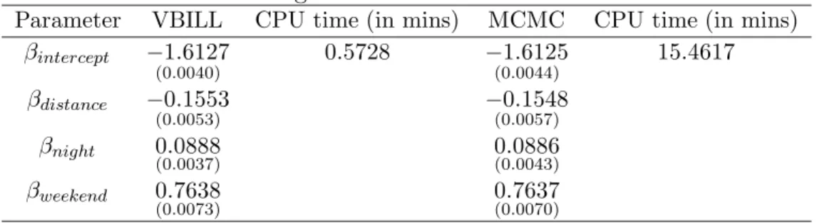
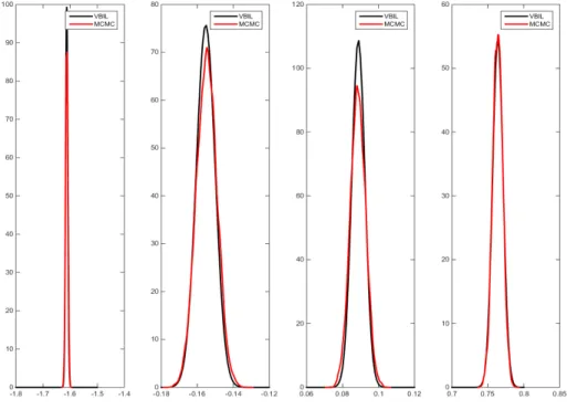
variance Vˆlm(θ) is given in Appendix 7.2. We set Vmax= 1000 in this example after some experiment. VBILL uses around 1% of the full one million observations on average at each iteration and converges within a few iterations. This example is run on a single desktop with 4 local processors. Table 1 shows the estimates of the posterior mean and posterior variance (shown in brackets) as well as the running time for both VBILL and MCMC methodologies. As shown, the VBILL estimates are very close to the “gold standard” MCMC estimates, but VBILL is 27 times faster than MCMC in this small data example. Figure 4.1 also shows that the posterior density estimates from VBILL and MCMC are very close to each other.
Table 1: Logistic Model Estimation Results
Parameter VBILL CPU time (in mins) MCMC CPU time (in mins) βintercept −1.6127 (0.0040) 0.5728 −1.6125 (0.0044) 15.4617 βdistance −0.1553 (0.0053) −(00.1548.0057) βnight 0.0888 (0.0037) 0.0886(0.0043) βweekend 0.7638 (0.0073) 0.7637(0.0070)
Figure 4.1: Comparisons of estimates of VBILL and MCMC for the Logistic model
We now run the VBILL for full dataset that exceeds the memory of a single desktop computer. We use the MapReduce programming technique in Matlab to process this big dataset. MapReduce is available in the R2014b release of Matlab. The MapReduce function requires three input arguments:
• A datastore function for reading the dataset into the “map” function in a chunk-wise fashion.
• A map function calculates the quantities of interest for each individual chunk of data. The MapReduce calls the map function one time for each chunk of the dataset stored in datastore.
• A reduce function aggregates outputs from the map function and produces final results.
We apply the MapReduce programming technique to estimate the log-likelihood unbiasedly. The datastore function splits the full dataset intoK chunks, each fits into the memory of a single desktop computer. The log-likelihood in equation (2.3) is decomposed correspondingly as l(θ) = K X k=1 l(k)(θ),
wherel(k) is the log-likelihood contribution based on data chunkk. Recall thatbl
m(θ)
is the unbiased log-likelihood estimator based on a random subset of size m from the full dataset. In the same vein, we denote by blmk(θ) the unbiased estimator of
l(k)(θ), based on a random subset of size m
k from data chunk k. The mk’s satisfy
m1+...+mK=m, typically mk=m/K. The map function is used to calculate the
chunk based estimate blmk(θ) for each chunk k in the same manner as described in Section 2.2. The reduce function aggregates all the chunk-based unbiased log-likelihood estimates into the full data based unbiased log-log-likelihood estimate
blm(θ) = K X k=1 blmk(θ). (4.1) It is obvious that Eblm(θ) =PKk=1Eblmk(θ) =PKk=1l(k)(θ) =l(θ). We note this
method is computer-memory efficient in the sense that the full dataset does not need to remain on-hold, and provides a highly efficient computational method for Big Data. It is important to note that our VBILL estimator is mathematically justified and independent of data chunking, as the estimatorblm(θ) in equation (4.1)
is guaranteed to be unbiased.
This example is run on an Intel Core i7 3.6 GHz desktop supported by the Matlab Parallel Toolbox with 4 local processors and the MapReduce built-in function. Given the maximum variance of the log-likelihood estimator Vmax= 1000, we use
approxi-mately 5% of the data in each subset. The VBILL algorithm converges within a few iterations. The CPU times taken to run the VBILL is 178.10 minutes. Although we use MapReduce to estimate the difference estimator and hence to obtain unbiased estimator of the log-likelihood so that the statistical properties of our estimator are still mathematically justified, we note that the time taken is a lot larger than the 1 million observations case. This is due to the communication cost between each data subset every time we estimate the difference estimator ˆdm. The communication
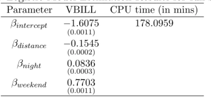
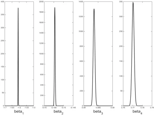
cost can be reduced by having a smaller number of subsets K. Figure 4.2 shows the marginal posterior density estimates of the parameters, which are bell shaped with very small variance as expected with a very large dataset. Table 2 shows the param-eter estimates from the logistic model for the full sample. This example confirms that the VBILL methodology with data subsampling and the difference estimator is useful for Bayesian inference in Big Data.
Table 2: Logistic Model Estimation Results for full sample
Parameter VBILL CPU time (in mins) βintercept −1.6075 (0.0011) 178.0959 βdistance −0.1545 (0.0002) βnight 0.0836 (0.0003) βweekend 0.7703 (0.0011)
Figure 4.2: Marginal Posterior Estimates for the Logistic model for the full sample
5
Application: Big Panel Data Models
In random effects panel data models withn panels{y1,...,yn}, the likelihood is
p(y|θ) = n Y i=1 p(yi|θ) = n Y i=1 Z p(yi|αi,θ)p(αi|θ)dαi. (5.1)
It is clear that with a very large number of panels, it is very expensive to compute the likelihood p(y|θ) at each value of θ. Here, the likelihood is intractable, but can be estimated unbiasedly using importance sampling (IS). Suppose that p(yi|θ) is
estimated unbiasedly by IS as b pnk(yi|θ) = 1 nk nk X j=1 wα(ij) , wα(ij) = pyi|α (j) i ,θ pα(ij)|θ gα(ij)|θ,yi , (5.2) whereα(ij)∼gα(ij)|θ,yi
forj= 1,..,nk and for some proposal density g(αi|θ,yi) such
that V(w)<∞ and nk is the number of important samples. However, in order to use the VBILL algorithm, we need an unbiased estimator of the log-likelihood contribution li(θ). It is clear that logpbnk(yi|θ) is a biased estimator of li(θ). This section describes two approaches to obtain unbiased or nearly unbiased estimators of the log-likelihoodli(θ).
5.1
Exact Debiasing Approach
General methods to obtain unbiased estimators from a sequence of biased estimators, referred to as “exact debiasing approach”, have been developed by McLeish (2012) and Rhee and Glynn (2015).
Letλ be an unknown constant that we want to estimate and let ζk, k= 0,1,...be
a sequence of biased estimators of λ, such that it is possible to generate ζk for each
k. We are interested in constructing an unbiased estimator λb of λ, i.e. E(bλ) =λ, based on the ζk’s, so that bλ has a finite variance. We now present the debiasing
approach, proposed independently by McLeish (2012) and Rhee and Glynn (2015), for constructing such a bλ. The basic idea is to introduce randomization into the sequence {ζk,k= 0,1,2,...}to eliminate the bias.
Proposition 1. [Theorem 1 of Rhee and Glynn (2015)]: Suppose that T is a non-negative integer-valued random variable such that P(T≥k)>0 for any k= 0,1,2,..., and that T is independent of the ζk’s. Let $k:= 1/P(T≥k). If
∞ X k=1 $kE (ζk−1−λ)2 <∞, (5.3) then b λ=ζ0+ T X k=1 $k(ζk−ζk−1) (5.4)
is an unbiased estimator of λ and has the finite variance
Vbλ= ∞ X k=1 $k E (ζk−1−λ)2−E (ζk−λ)2 −E (ζ0−λ)2 <∞. (5.5) Unbiased estimators obtained using current debiasing approach can take negative values with a positive probability, even if their expectations are known to be non-negative. See Jacob and Thiery (2015) for a detailed discussion. This debiasing estimator may not be suitable for PMMH and VBIL since they require that the likelihood estimator must be non-negative almost surely.
Although bλ is an unbiased estimator of λ, its variance can be large. We can reduce this variance by averaging over replications of λb, bλ=bλ1+...+bλnrep
/nrep, with the λbi independent replications of bλ. Doing this also gives us an estimate of
Vλb, b Vλˆ= 1 nrep−1 nrep X i=1 ˆ λi−λˆ 2 .
Then Vbbλ=Vbbλ/nrep is an estimator of the variance of bλ.
We now apply this exact debiasing approach to obtain unbiased estimators ˆli(θ)
of li(θ). Assume that the proposal density g in equation (5.2) is sufficiently heavy
tailed so that
σi2(θ) =
V(w)
p(yi|θ)2
Then i,nk:= √ nk b pnk(yi|θ) p(yi|θ) − 1 /σi(θ)
has zero mean and unit variance, and is approximately normal N(0,1) as nk grows.
Letζk= logpbnk(yi|θ), ζk−li(θ) = log 1+σi(θ)i,nk √n k = σi(θ)i,nk √n k − σ2 i(θ)2i,nk 2nk +σ 3 i(θ)3i,nk 3nk√nk +... (5.6) So (ζk−li(θ))2= σ2 i(θ)2i,nk nk − σ3 i(θ)3i,nk nk√nk +... (5.7) Therefore, when nk is large enough
E (ζk−li(θ))2 =σ 2 i(θ) nk +o n−1 k .
Letτ be a number such that 0< τ <1. Define
nk=d
1
τkPr(T≥k+1)e (5.8)
withdxebeing the smallest integer that is larger than or equal tox. Then, condition (5.3) is satisfied. Therefore, ˆli(θ) :=ζ0+ T X k=1 $k(ζk−ζk−1) is an unbiased estimator of li(θ).
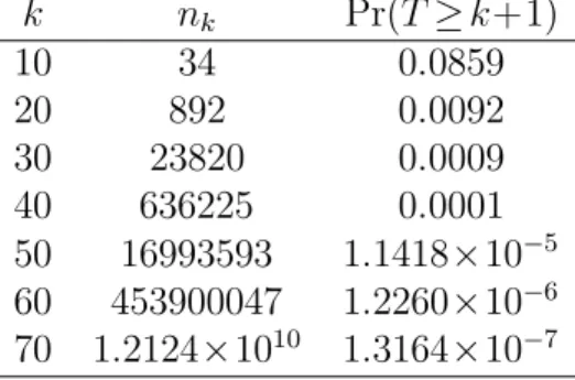
Choosing Distribution for T. A possible choice of the distribution of T is a negative binomial distribution Pr(T=k) =ρ(1−ρ)k, k= 0,1,... for 0< ρ <1. Then
$k= 1/Pr(T≥k) = 1/(1−ρ)k. The number of importance samples nk for each of the
ζk from equation (5.8) is
nk=d
1
τk(1−ρ)k+1e.
Ifk is large, thennk can be so large that it can freeze the computer. Table 3 shows
the number of importance samplesnk for differentkand the probability Pr(T≥k+1)
when τ= 0.9 and ρ= 0.2. When k= 40, nk is too large to handle and it happens
once every 10000 iterations. It is important to make nk increase slowly while the
condition in Proposition 1 is still guaranteed. One way to solve this problem is by constructing the distributionT carefully.
Table 3: nk when τ= 0.9 andT is negative binomial with parameters 1 and ρ= 0.2 k nk Pr(T≥k+1) 10 34 0.0859 20 892 0.0092 30 23820 0.0009 40 636225 0.0001 50 16993593 1.1418×10⁻⁵ 60 453900047 1.2260×10⁻⁶ 70 1.2124×10¹⁰ 1.3164×10⁻⁷
In Proposition 1, T can be any non-negative integer-valued random variable such that Pr(T ≥k)>0 for any k= 0,1,2,.... The idea here is to construct distribution
T such that the number of important samples nk increases slowly and is not too
large to handle computationally. We propose one possible approach to construct such distribution. We define the distribution of T as a mixture:
Pr(T=k) =wPr(T1=k)+(1−w)Pr(T2=k).
LetK be a reasonably large number, but not too large for computational cost con-sideration. The idea here is to use the K biased estimators ζ1,...,ζK to build the
unbiased estimators ˆli(θ). The first distribution Pr(T1=k) is truncated so that its
values lie within the interval [0,K]. The distribution of T1 is given by:
Pr(T1=k) = ( 1 k1+β/ PK l=1l1+1β, k= 1,...,K 0 k > K and Pr(T1≥k)= 1−Pkh−=11 1 h1+β PK l=1l1+1β , k= 1,...,K 0 k > K
where β is small, for example 0.01. The distribution of T2 is negative binomial
distributionNB(1,ρ), whereρ is chosen such that the probability of getting largek
is very small. So,
Pr(T≥k) = wPr(T1≥k)+(1−w)Pr(T2≥k)
= wPr(T1≥k)+(1−w)(1−ρ)k.
The nk can be computed using the following formula
nk=d
1
τkwPr(T
1≥k+1)+(1−w)(1−ρ)k+1
e
for some values of 0< τ <1. The first component in the denominator controls the rate of nk. Without this component, nk increases exponentially. Table 4 shows the
τ=0.95, ρ=0.99, w=0.9,K=20, andβ=0.01. Using this setup,T still has a chance of being K, then
nK=d
1
τK(1−w)(1−ρ)K+1e
can be large. We can define nK=nK−1 and condition (5.3) still holds.
Table 4: nk when K= 20, w= 0.9,τ= 0.95, ρ= 0.99, β= 0.01 k nk Pr(T1≥k+1) Pr(T2≥k+1) Pr(T≥k+1) 5 4 0.3613 10−12 0.3251 10 11 0.1832 10−22 0.1649 19 216 0.0137 10−40 0.0123 20 2.7895e+43 0 10−42 10−43
5.2
Taylor Correction Approach
Although the exact debiasing approach provides us with an exactly unbiased esti-mator of the log-likelihood, the estiesti-mator might have a high variance and be com-putationally expensive to compute. A fast alternative is to use the Taylor correction approach. From equation (5.6), i,n∼ N(0,1) as n is large, so E 3i,n
≈0 and thus, E(logˆpn(yi|θ)−li(θ)) =−σ2i(θ) 2n +O n −2, where σ2 i(θ) =nV(ˆpn(yi|θ))/p(yi|θ)2. Therefore, eli(θ) := log ˆpn(yi|θ)+b σ2 i(θ) 2n is an
ap-proximately unbiased estimator of li(θ) with a bias of order n−2. Although this
method only provides us with a nearly unbiased estimator of li(θ), the bias term
decreases to zero very fast with the number of samplesn and the variance ofeli(θ) is
in general much smaller than the variance of the exact unbiased estimatorbli(θ).
5.3
Simulation Study: Random Effects Panel Data Model
The proposed VBILL estimator with data subsampling and the difference estimator is written in Matlab. The examples with moderate data are run on an Intel Core i7 3.6 GHz desktop supported by the Matlab Parallel Toolbox with 4 local processors. The bigger data example is run on a high performance cluster with 12 local processors. The performance of VBILL with data subsampling and the difference estimator is compared to pseudo-marginal MCMC (PMMH) simulation (Andrieu and Roberts (2009)), which still generates samples from the posterior when the likelihood in the Metropolis-Hastings algorithm is replaced by its unbiased estimator. The likelihood in the panel data context is a product of n integrals over random effects. Each integral is estimated unbiasedly using importance sampling (IS), with the number of importance samples chosen such that the variance of unbiased likelihood estimator is approximately 1, for the optimal PMMH as suggested by Pitt et al. (2012). Each MCMC chain consists of 30000 iterates with another 10000 iterates used as burn in iterates.Panel data are generated from the following logistic model with random effects:
p(yit|β, αi) =Binomial(1, pit),
and
Logit(pit) =β0+β1xit+αi (5.9)
for i= 1,...,n and t= 1,...,5, αi∼N(0,τ2). For the moderate simulation study, we
generate two datasets of n= 400 and n= 1000, and β= (−1.5,1.5)0, τ2= 1.5, and
xit∼U(0,1).
We use the variational distributionqλ(θ)=q(β)q(τ2), whereq(β) is ad=2-variate
normal N(µ,Σ) and q(τ2) is an inverse gamma distribution IG(a,b). We then run
VBILL with data subsampling and difference estimator for both exact debiasing and the Taylor correction approach. For the difference estimator,wi(θ)≡logbp yi|θ
, with
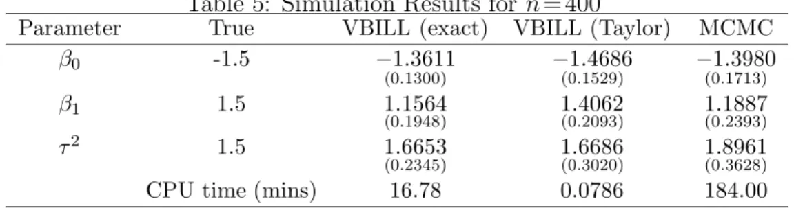
θ a simulated maximum likelihood (SML) estimate of θ. Table 5: Simulation Results forn= 400
Parameter True VBILL (exact) VBILL (Taylor) MCMC
β0 -1.5 −1.3611 (0.1300) −(01.4686.1529) −(01.3980.1713) β1 1.5 1.1564 (0.1948) 1.4062(0.2093) 1.1887(0.2393) τ2 1.5 1.6653 (0.2345) 1.6686(0.3020) 1.8961(0.3628)
CPU time (mins) 16.78 0.0786 184.00
Table 6: Simulation Results for n= 1000
Parameter True VBILL (exact) VBILL (Taylor) MCMC
β0 -1.5 −1.5205 (0.1104) − 1.5514 (0.0939) − 1.4694 (0.1021) β1 1.5 1.6619 (0.1565) (01.6722.0.1445) 1.6228(0.1553) τ2 1.5 1.3853 (0.1375) 1.2724(0.1670) 1.4580(0.1824)
CPU time (mins) 22.8204 0.0647 1330
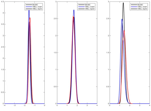
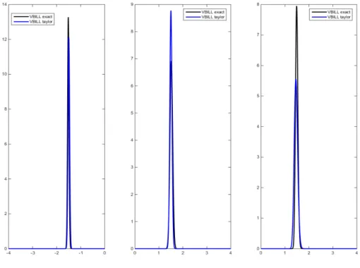
Tables 5 and 6 show the estimates of the posterior mean and posterior variance (shown in brackets) ofβ0,β1, andτ2 for the three methodologies MCMC, VBILL with
exact debiasing, and VBILL with the Taylor series correction. All the estimates are close to their true values. In Table 5 where n= 400, VBILL seems to underestimate the posterior variances compared to the “gold standard” MCMC estimates, while in Table 6 where n= 1000, VBILL estimates the variance more accurately. Figure 5.1 and 5.2 plot the VBILL estimates and MCMC estimates of the marginal posteriors
π(β0), π(β1), andπ(τ2). These two figures show that the VBILL marginal posterior
estimates using both the bias correction approaches are very close to the MCMC estimates especially when the number of panels is 1000. This confirms that with a large number of panels or observations and a small number of parameters, we know that the posterior π(θ) is approximately normal, so the VBILL variational distribution q(β) =N(µ,Σ) should be a very accurate approximation of π(θ) as can be seen from Figure 5.2.
We note that the VBILL with the exact debiasing approach takes a much longer time to run compared to VBILL with Taylor correction, with a not much difference in the resulting marginal posterior estimates. On average at each iteration, VBILL with exact debiasing and with the Taylor series correction use around 8% and 1.5% of the full dataset, respectively. The variance of the exactly unbiased estimator is large in this example so it is computationally more expensive to reduce the variance toVmax.
Figure 5.2: Simulation Results for n= 1000 panels
Large Panel Data Example
This section describes a scenario where it is difficult to use the PMMH method. We consider a large data case with the number of panels n= 10000. The PMMH method will not work since the variance of unbiased estimator of the likelihood is very large and it requires a huge number of importance samples in order to target the optimal variance of 1. So, if an optimal PMMH procedure is run on our computer to generate 40000 iterations, it would take 124,530 minutes. We run the VBILL based on the exact debiasing and Taylor correction, with the maximum variance Vmax set
to 5000 and 1000, respectively, which require approximately 20% and 5% of the full dataset on average in each iteration of the VBILL procedure. This is because the exact debiasing approach produces an unbiased estimator of the log-likelihood with a larger variance, thus it requires a bigger subsample size to keep the variance below the maximum variance. Both VBILL methods converge after a few iterations. Table 7 summarizes the results. Figure 5.3 plots the variational approximations of the marginal posteriors, which are bell shaped as expected with a very large dataset. The two debiasing correction approaches produce very similar results, however, the CPU time for VBILL with the Taylor correction is much smaller than the VBILL with the exact debiasing approach. This makes VBILL with the Taylor correction suitable for the big panel data models.
Table 7: Simulation results: large dataset application to the logistic model with random effects)
Parameter True VBILL (exact) VBILL (Taylor)
β0 -1.5 −1.5166 (0.0301) −(01.4940.0329) β1 1.5 1.5174 (0.0577) 1.5002(0.0455) τ2 1.5 1.4917 (0.0025) 1.4618(0.0052)
CPU time (in mins) 452.43 1.18
Figure 5.3: Simulation results: large dataset application to the logistic model with random effects
6
Conclusions
We have proposed the VBILL algorithm with data subsampling and the difference estimator, which is useful for Bayesian inference in big data and big panel data models. For panel data examples, our proposed algorithms, especially the VBILL algorithm with the Taylor series correction, are much faster than PMMH and produce estimates that are very close to PMMH. Furthermore, the proposed methodology works well when the log-likelihood estimates are highly variable. We also make use of the advanced MapReduce programming technique to develop an approach to analyse massive datasets which cannot fit into a single desktop’s memory. Our estimator is mathematically justified and independent of data chunking.
7
Appendix
7.1
Variance Reduction Methods
The performance of Algorithm 1 depends greatly on the variance of the noisy gradi-ent. This section describes control variate methods to reduce this variance.
Control Variate
Denote bh(θ,γ) := logp(θ)+bl(θ,γ) and let θs∼qλ(θ) and γs∼g(γ|θs) for s= 1,...,S, be
S samples from the variational distributionqλ(θ)g(γ|θ). For any numberci, consider
\ ∇λiKL(λ) = 1 S S X s=1 ∇λi(logqλ(θs)) logqλ(θs)−bh(θs,γs)−ci
which is still an unbiased estimator of ∇λiKL(λ), whose variance can be reduced by an appropriate choice of ci. Similar ideas are considered in the literature; see Tran
et al. (2015), Paisley et al. (2012); Ranganath et al. (2014). The optimal ci that
minimizes the variance of ∇\λiKL(λ) is given by,
ci= cov∇λi(logqλ(θ)) logqλ(θ)−bh(θ,γ) ,∇λi(logqλ(θ)) V(∇λi(logqλ(θ))) , (7.1) which can be estimated by samples (θs,γs)∼qλ(θ,γ). The samples used to estimate
ci must be independent of the samples used to estimate the gradient to ensure the
unbiasedness of the gradient estimator. In practice, the ci can be updated
sequen-tially as follows. At iterationt, we use theci computed in the previous iterationt−1
to estimate the gradient ∇\λiKL λ
(t), which is estimated using new samples from
qλ(t)(θ,γ). We then update the ci using this new set of samples. Doing this reduces
computational cost since no extra samples are needed to be generated in updating
ci and the unbiasedness of the gradient estimator is achieved.
Exponential Family and Natural Gradient
Suppose that the variational distribution qλ(θ) belongs to an exponential family of
the form,
qλ(θ) = exp
T(θ)0λ−Z(λ),
whereT(θ) is the vector of sufficient statistics and λis vector of natural parameters. Then, as shown in Tran et al. (2015),
∇λKL(λ) =IF(λ)λ−H(λ). Here H(λ) =Eθ,γ b h(θ,γ)∇λ(logqλ(θ))
and IF(λ) = covqλ(T(θ),T(θ)) is the Fisher information matrix and can be computed in closed form in most cases. The vector
method can be used to reduce the variation in estimating H(λ). Given S samples (θs,γs), the ith element is estimated unbiasedly by:
b Hi(λ) = 1 S S X s=1 bh(θs,γs)−ci ∇λi(logqλ(θ)), where ci=
covbh(θ,γ)∇λi(logqλ(θ)),∇λi(logqλ(θ))
V(∇λ
i(logqλ(θ)))
.
Using the natural gradient in minimising the Kullback-Leibler divergence is in general more efficient and reliable than the traditional gradient (Amari, 1998; Tran et al., 2015). If the variational distribution qλ(θ) has the exponential family form, the
natural gradient is given by
∇λKL(λ)natural=λ−IF(λ)−1H(λ).
Using the natural gradient, and assuming that the variational distributionqλ(θ) has
the exponential family form, the algorithm 1 becomes,
Algorithm 2. • Initialize λ(0) and stop the following iteration if the stopping
criterion is met.
• For t= 0,1,..., compute λ(t+1)= (1−a
t)λ(t)−atIF λ(t)
−1b
H λ(t).
7.2
Estimating the variance of the unbiased log-likelihood
estimator
b
l
m(
θ
)
The estimator of the log-likelihood from a data subsample of sizemis of the following form, blm(θ) =w+dbm, dbm= 1 m m X i=1 ndui
with ui independently and uniformly distributed on the index set{1,...,n}. So
Vblm(θ)=V(dbm) = n2 mV(dui) = n2 mσ 2 pop, where σpop2 = 1 n n X i=1 d2i − 1 n n X i=1 di !2
can be considered as the population variance of the entire population {d1,...,dn}.
Given observations {du1,...,dum}, this population variance can be estimated by the sample variance b σ2pop= 1 m−1 m X j=1 duj − 1 m m X i=1 dui !2 = 1 n2(m−1) m X j=1 nduj −dbm 2 .
The variance ofblm(θ) is estimated by
b Vblm(θ)= n2 mbσ 2 pop= 1 m(m−1) m X j=1 nduj −dbm 2 .
7.3
Proof of Theorem 1
Proof of Theorem 1. (i) Algorithm 1 is the Robbins-Monro procedure for finding the root λ∗ of the equation ∇
λKL(λ) = 0. So (3.1) follows from Theorem 1 of Sacks
(1958).
(ii) We denote by ∇^λKL(λ∗) the noisy gradient obtained when the log-likelihood is
available. Then, noting that E∗(ζ∗(θ)) = 0, the constant cin (7.1) is c=Eθ,γ{ζ∗(θ) 2(logq λ∗(θ)−logp(θ)−bl(θ, γ))} E∗ζ∗(θ)2 = E∗{ζ∗(θ)2(logq λ∗(θ)−logp(θ)−l(θ))} E∗ζ∗(θ)2 =ec.
We note that ec is the control variate constant we would use to compute ∇^λKL(λ∗)
if the log-likelihood was known. By the law of total variance, V \∇λKL(λ∗) = 1 SVθ,γ n ζ∗(θ)(logqλ∗(θ)−logp(θ)−bl(θ, γ)−c) o = 1 SE∗ n ζ∗2(θ)σ2(θ)o+ 1 SV∗ n ζ∗(θ)(logqλ∗(θ)−logp(θ)−l(θ)−c) o = 1 SE∗ n ζ∗2(θ)σ2(θ)o+ 1 SV∗ n ζ∗(θ)(logqλ∗(θ)−logp(θ)−l(θ)−ec) o = 1 SE∗ n ζ∗2(θ)σ2(θ)o+V ^∇λKL(λ∗) . Therefore, σasym2 (bλM) =cλ∗V \∇λKL(λ∗) =σasym2 (eλM) + cλ∗ S E∗ n ζ∗2(θ)σ2(θ) o .
References
Amari, S. (1998). Natural gradient works efficiently in learning. Neural computation, 10(2):251–276.
Andrieu, C. and Roberts, G. (2009). The pseudo-marginal approach for efficient Monte Carlo computations. The Annals of Statistics, 37:697–725.
Battey, H., Fan, J., Liu, H., Lu, J., and Zhu, Z. (2015). Distributed estimation and inference with statistical guarantees. Technical report. arXiv:1509.05457v1. Bishop, C. M. (2006). Pattern Recognition and Machine Learning. New York:
Springer.
Fitzmaurice, G. M., Laird, N. M., and Ware, J. H. (2011). Applied Longitudinal Analysis. John Wiley & Sons, Ltd, New Jersey, 2nd edition.
Flury, T. and Shephard, N. (2011). Bayesian inference based only on simulated like-lihood: Particle filter analysis of dynamic economic models. Econometric Theory, 1:1–24.
Hoffman, M. D., Blei, D. M., Wang, C., and Paisley, J. (2013). Stochastic variational inference. Journal of Machine Learning Research, 14:1303–1347.
Jacob, P. and Thiery, A. H. (2015). On non-negative unbiased estimators. Annals of Statistics, 43(2):769–784.
Kane, M. J., Emerson, J., and Weston, S. (2013). Scalable strategies for computing with massive data. Journal of Statistical Software, 55 (14):1–19.
McLeish, D. (2012). A general method for debiasing a Monte Carlo estimator. Monte Carlo Methods and Applications, 17:301–315.
Nott, D. J., Tran, M. N., and Leng, C. (2012). Variational approximation for het-eroscedastic linear models and matching pursuit algorithm. Statistics and Com-puting, 22(2):497–512.
Ormerod, J. T. and Wand, M. P. (2010). Explaining variational approximations. American Statistician, 64:140–153.
Paisley, J., Blei, D., and Jordan, M. (2012). Variational Bayesian inference with stochastic search. In International Conference on Machine Learning, Edinburgh, Scotland, UK.
Pitt, M. K., Silva, R. S., Giordani, P., and Kohn, R. (2012). On some properties of Markov chain Monte Carlo simulation methods based on the particle filter.Journal of Econometrics, 171(2):134–151.
Quiroz, M., Villani, M., and Kohn, R. (2015). Scalable MCMC for large data prob-lems using data subsampling and the difference estimator. Technical report, Stock-holm University. http://arxiv.org/abs/1507.02971v2.
Ranganath, R., Gerrish, S., and Blei, D. M. (2014). Black box variational inference. In International Conference on Artificial Intelligence and Statistics, volume 33, Reykjavik, Iceland.
Rhee, C. H. and Glynn, P. W. (2015). Unbiased estimation with square root conver-gence for sde model. Operation Research, 63(5):1026–1043.
Sacks, J. (1958). Asymptotic distribution of stochastic approximation procedures. The Annals of Mathematical Statistics, 29(2):373–405.
Sato, M. (2001). Online model selection based on the variational Bayes. Neural Computation, 13(7):1649–1681.
Tran, M.-N., Nott, D., and Kohn, R. (2015). Variational Bayes with intractable likelihood. Technical report, University of Sydney. arXiv:1503.08621.
Wang, C., Chen, M. H., Schifano, E., Wu, J., and Yan, J. (2015). A survey of statis-tical methods and computing for big data. Technical report. arXiv:1502.07989v1.