Bayesian inference for quantiles and conditional means in log-normal models

(1)

Alma Mater Studiorum

Università di Bologna

DOTTORATO DI RICERCA IN SCIENZE STATISTICHE CICLO XXXII Settore Concorsuale: 13/D1 Settore Scientico Disciplinare: SECS-S/01

Bayesian inference for quantiles and

conditional means in log-normal models

Presentata da: Aldo Gardini

Coordinatrice Dottorato: Supervisor:

Prof.ssa Alessandra Luati Prof. Carlo Trivisano

(2)

(3)

Abstract

The main topic of the thesis is the proper execution of a Bayesian inference if log-normality is assumed for data. In fact, it is known that a particular care is required in this context, since the most common prior distributions for the variance in log scale produce posteriors for the log-normal mean which do not have nite moments. Hence, classical summary measures of the posterior such as expectation and variance cannot be computed for these distributions.

The thesis is aimed at proposing solutions to carry out Bayesian inference inside a mathematically coherent framework, focusing on the estimation of two quantities: log-normal quantiles (rst part of the thesis) and conditioned expec-tations under a general log-normal linear mixed model (second part of the thesis). Moreover, in the latter section, a further investigation on a unit-level small area models is presented, considering the problem of estimating the well-known log-transformed Battese, Harter and Fuller model in the hierarchical Bayes context. Once the existence conditions for the moments of the target functionals pos-terior are proved, new strategies to specify prior distributions are suggested. Then, the frequentist properties of the deduced Bayes estimators and credible intervals are evaluated through accurate simulations studies: it resulted that the proposed methodologies improve the Bayesian estimates under naive prior set-tings and are satisfactorily competitive with the frequentist solutions available in the literature. To conclude, applications of the developed inferential strategies are illustrated on real datasets.

The work is completed by the implementation of an R package named BayesLN which allows the users to easily carry out Bayesian inference for log-normal data.

(4)

List of Figures

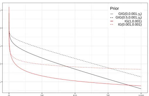
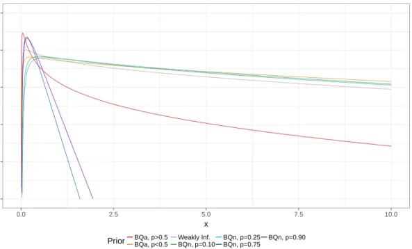
1.1 Plot of the density function of a log-normal distribution with ξ = 0 and dierent values ofσ2_{. . . 10} 2.1 Plots of the GIG density function with dierent values of the parameters. . . 19 2.2 Comparison SMNG density and log-density changing the parameters. . . 24 2.3 Plots of GH and SMNG densities with the same parameters . . . 28 3.1 Log density of the weakly informative GIG distributions proposed and of the

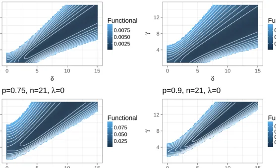
most common vague inverse gamma (IG) priors. . . 42 3.2 Behaviour of the target functional for _θˆQB

p with respect to the parameters γ andδ . . . 44 3.3 Behaviour of thetarget functional for _θˆQB

0.5 and θˆ RQB

0.5 with respect to the pa-rametersγ andδ. . . 45 3.4 Comparison of log-densities of dierent GIG priors. A random sample of size

n= 21generated from a log-normal having σ2 _{= 0}_.₅_{is used. . . 47} 4.1 Comparison between the at improper prior onξ(dashed lines) and the NGIG

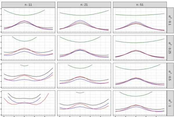
prior (solid lines). The changes of the CRMSE and relative bias with respect toξ0 are shown for the scenarios withn= 11andn= 21withσ2 = 0.5. The results for quantiles0.1,0.5and 0.9are reported. . . 60 4.2 Comparison at the dierent quantile levels among the considered estimators

in terms of CRMSE and RB. For the sample sizes of 11 and 21 the variance is xed equal to 0.25, 0.5, 1. . . 66 4.3 Kernel density plots of the posterior standard deviation distributions of the

ˆ

θBn p and θˆ

QBa

p estimators at dierent quantiles p. The case σ2 = 0.5 and

n = 21 is reported. The vertical lines show the square root of the Monte Carlo variances averages of the estimators . . . 67 4.4 Average width of the Bayesian credible interval compared to the frequentist

condence interval. The trend with respect to the sample size n is reported at dierent quantiles p. . . 72 4.5 Relative RMSE and relative bias of various estimators of the target quantity

θp(˜x), withp= 0.10. . . 74

(8)

4.6 Relative RMSE and relative bias of various estimators of the target quantity θp(˜x), withp= 0.50. . . 75 4.7 Relative RMSE and relative bias of various estimators of the target quantity

θp(˜x), withp= 0.90. . . 76 4.8 Frequentist coverages of the credible intervals. The nominal coverage is0.90. . 77 4.9 Average widths of the Bayesian credible intervals at dierent quantiles and

combinations ofσ2 _and _n_{. . . 78} 4.10 Comparison between the distributions obtained in the three dierent Bayesian

approaches adopted for the example in environmental monitoring. . . 80 4.11 Comparison between the distributions obtained in the three dierent Bayesian

approaches adopted for the example about lifetime data. . . 84 4.12 Posterior distribution of the median estimator in the example about lifetime

data. . . 85 4.13 Posterior density of the regression coecient β1 under dierent prior

distri-butions for the varianceσ2_{. . . 88} 4.14 Estimated conditional quantiles of the annual peak ow with dierent

meth-ods and dierent probability levels. The shaded area represents the 90% credible interval for the weakly informative prior setting. . . 89 6.1 Trends of the mean estimate, RMSE, frequentist coverage and average interval

width are reported for each area and for the three considered scenarios. . . . 126 6.2 Traceplots of the overall mean θm under the three priors considered for the

whole dataset (left) and for the sub-sample of the rst6 workers (right). . . . 129 A.1 Curve of the Bessel K function with dierent ordersν. . . 142 D.1 Relative RMSE and relative bias of various estimators of the target quantity

θp(x0), withp= 0.25. . . 151 D.2 Relative RMSE and relative bias of various estimators of the target quantity

θp(x0), withp= 0.75. . . 152 D.3 Relative RMSE and relative bias of various estimators of the target quantity

(9)

List of Tables

1.1 Results of the MCMC exercise involving the estimation of mean (θ1,0.5), me-dian (θ0.5) and quantiles (θ0.1,θ0.9) for the toy example. . . 13 1.2 Results of the MCMC exercise involving the estimation of global mean (θm)

and group means (θc(νl)) under a one way random eect ANOVA model, considering the toy dataset. . . 14 4.1 RRMSE and RB for the estimator of quantile p = 0.1. θˆ_0.1QBn is subjected to

dierent prior settings onξ. . . 57 4.2 RRMSE and RB for the estimators of quantilep= 0.5. θˆ_0.5QBnand θˆ_0.5RQBw are

subjected to dierent prior settings onξ. . . 58 4.3 RRMSE and RB for the estimator of quantile p = 0.9. θˆ_0.9QBn is subjected to

dierent prior settings onξ. . . 59 4.4 RRMSE and RB for Bayes estimators of quantiles 0.05 and 0.25. A guesss2

0 ofσ2 _{is included in the choice of the hyperparameters. . . 61} 4.5 Root MSE and relative bias for Bayes estimators of quantile 0.75 and 0.95.

A guesss2

0 of σ2 is included in the choice of the hyperparameters. . . 62 4.6 RRMSE and RB of estimators for θp with respect to dierent sample sizesn

and quantilesp, with σ2 _{= 0}_.₂₅_{. . . 64} 4.7 RRMSE and RB of estimators for θp with respect to dierent sample sizesn

and quantilesp, withσ2 _{= 1}_{. The Bayes estimator}_θˆB

p is the estimator under relative quadratic loss for the median and the one under quadratic loss for the others. . . 65 4.8 Monte Carlo standard deviation of the estimator _θˆBn

p in the sample space and square root of the expectation of the posterior variance distribution at dierentn,σ2_,_p_{. . . 68} 4.9 Performances of dierent estimators of the target functional θp in case of

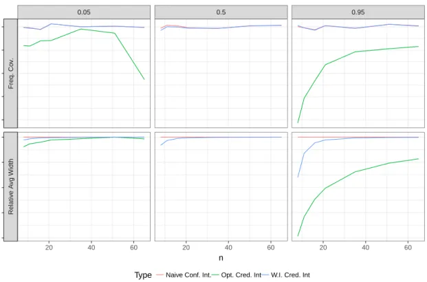
misspecied log-normal distribution. Dierent generating distribution and various samples sizes are considered. . . 70 4.10 Comparison between the condence interval (Conf. Int.) and the Bayesian

credible interval (Cred. Int.) in terms of coverage (Cov.), with the nominal level xed at0.95, and average width. Dierent combinations ofσ2 _and _n_at dierent quantiles are reported. . . 71

(10)

4.11 Point estimates of θ0.95with dierent methods. The standard error estimates are reported too if available. . . 79 4.12 Estimates of θ0.95with dierent methods: naive (θˆ0.95), Longford (Qˆ0.95), the

Bayes estimators under weakly informative prior (_θˆQBw

0.95 ), MSE-optimizing prior (_θˆQBn

0.95 ) and the approximately optimal prior (θˆ QBa

0.95). . . 83 4.13 Estimates of θp with dierent methods atp∈ {0.01,0.1,0.5}. The estimates

of the standard errors are reported. . . 85 4.14 Condence intervals and credible intervals (95%): LCL for the quantiles0.01

and0.1, two sided for the median. . . 86 4.15 Estimates of θp with dierent methods at p ∈ {0.80,0.90,0.98,0.99}. The

estimates of the standard errors are reported. . . 87 6.1 Bias and RMSE for the considered estimators of θm in the dierent scenarios. 121 6.2 RABias and RRMSE for the considered estimators of the group-specic

ex-pectations in the dierent scenarios. . . 122 6.3 Coverage and average width for the credible intervals of θm and averaged for

the group-specic expectations. . . 123 6.4 For each scenario, the estimates properties averaged with respect to areas

having the same sample size nd are reported for the dierent methods con-sidered. . . 127 6.5 Averaged RRMSE and bias obtained with the EB and HB with GIG prior

methods using the AAGIS data for design-based simulation. . . 128 6.6 Point estimates and posterior standard deviations (for Bayesian methods) of

the model parameters, global expectation and conditioned expectations are reported for both the analysis carried out on the complete dataset and the reduced one. . . 130 6.7 Point estimates and posterior standard deviations (for Bayesian method) of

the model parameters and the target expectations are reported. . . 136 D.1 Root MSE and relative bias of estimators for θp with respect to dierent

sample sizes n and quantiles p, with σ2 _{= 0}_.₅ _{. The Bayes estimator} _θ_ˆB p is the estimator under relative quadratic loss for the median and the one under quadratic loss for the others. . . 149 D.2 Root MSE and relative bias of estimators for θp with respect to dierent

sample sizes n and quantiles p, with σ2 _{= 2} _{. The Bayes estimator} _θ_ˆB p is the estimator under relative quadratic loss for the median and the one under quadratic loss for the others. . . 150 D.3 Frequentist properties of the estimators_θˆB,GIG

m andθˆB,GIGc (νj)obtained with GIG priors havingλ= 0.5. . . 154 D.4 Frequentist properties of the estimators_θˆB,GIG

m andθˆB,GIGc (νj)obtained with GIG priors havingλ= 2. . . 155

(11)

Introduction

The use of the logarithmic transformation in statistics has a long tradition. One of its main applications is the normalization of samples for which the Gaussian assumption is unreliable in the original scale. In fact, after the introduction of the analysis of variance method, whose starting point could be considered the paper by Fisher and Mackenzie (1923), the necessity to generalize this revolutionary technique to non-normal data emerged. In this sense, the log-transformation appears in the paper by Cochran (1938) among other transformations aimed at making experimental data suitable to apply the analysis of variance method, i.e. homoscedasticity and normality (with a particular focus on skewed distributions). In this paper, Cochran writes: The transformation to logs. equalizes the variance when it is pro-portional to the square of the mean; it is thus a much more powerful transformation than the square root or the inverse sine.

Another example of early use of the logarithmic transformation by applied scientists is the paper by Williams (1937). He focuses on the fact that log-transforming the data is appealing when the the goal of the statistical analysis is the estimation of the geometric mean: back-transforming the arithmetic mean estimated on the log-transformed data, an estimate of the geometric mean of the original data is obtained (McAlister, 1879). Few years later, a dierent perspective of the idea of data transformation is provided in the paper by Finney (1941), that could be seen as the starting point of the inference on log-normal distribution. In eect, he noted that, if the log-transformation is performed, then a crucial step of the inferential procedure is represented by the back-transformation to the original data scale. In particular, he presented the rst proposal of an ecient estimator for the arithmetic mean of the original data, exploiting the properties of the log-normal distribution.

The popularity of the log-transformation further increased thanks to the well known proce-dure introduced by Box and Cox (1964). In fact, the logarithm represents a particular case of the proposed data transformation algorithm.

Unfortunately, in applied sciences (but also among statisticians), there is a huge misunder-standing about the adoption of the logarithmic transformation in data analysis. Probably, the main source of confusion is represented by the following wrong procedure: (1) transform-ing the data, (2) applytransform-ing the well-known normal methods on the log-transformed sample and

(12)

then (3) naively back-transform the results to the original data scale, ignoring basic concepts as Jensen's inequality. On the other hand, if the real interest of the analysis is to produce inference about key quantities of the original data scale (i.e. the scale of the untransformed data), then the idea of transformation should be abandoned, passing to the more coherent idea of carrying out a proper and careful inference on skewed data whose logarithm is nor-mally distributed (Finney, 1941), and the log-normal (Crow and Shimizu, 1987) distribution might represent a convenient assumption.

This particular distribution is frequently used in several applied elds like economics, envi-ronmental sciences, biostatistics and engineering, in order to analyse dierent kind of data (Limpert et al., 2001).

1.1 The log-normal distribution

0.0 0.2 0.4 0.6 0.8 0 2 4 6 x f(x) σ2_: ₂ ₁ _0.5

Figure 1.1: Plot of the density function of a log-normal distribution withξ= 0and dierent values

ofσ2_.

A brief overview of the log-normal distribution is provided in order to introduce the pro-tagonist of this thesis and to x the notation. If a random variableX is assumed normally distributed:

X ∼ N ξ, σ2

, (1.1)

(13)

distributed:

Z _∼log_N(ξ, σ2). (1.2)

The probability density function (gure 1.1) is: fZ(z) = √ 1 2πσz exp − 1 2σ2(logz−ξ) 2 , z >0. (1.3)

The family of functionals which includes the most important quantities that characterize the distribution is:

θa,b= exp

aξ+bσ2 . (1.4)

It provides the arithmetic mean if a= 1, b = 0.5; the median when a= 1, b = 0 and the mode with a= 1, b =₋1. More generally, each raw moment can be expressed choosing a couple of values fora andb.

On the other hand, the functional that denes the quantiles of the log-normal distribution is the following:

θp= exp

ξ+ Φ−1₍_p₎_σ _, _(1.5)

whereΦ−1₍_p₎_{is the inverse of the standard normal cumulative distribution function, i.e. the}

p-th quantile of the standardized Gaussian distribution which corresponds to probabilityp. To complete the general characterization of the distribution, the variance of a log-normal random variable is:

V[Z] =

eσ2−1e2ξ+σ2, (1.6)

from which follows that the coecient of variation does not depend on the mean in the log-scaleξ:

CV[Z] =peσ2

−1. (1.7)

Finally, another useful quantity to report is the distribution skewness:

eσ2 + 2 peσ2

−1. (1.8)

1.2 Log-normal distribution in Bayesian inference: a

motivat-ing example

As outlined before, one of the most critical points of making inference with the log-normal assumption is the back-transformation of the results which are obtained in the Gaussian framework to the original data scale, without neglecting the achievement of ecient estima-tors.

The study of appropriate and ecient estimators for crucial quantities related to the log-normal distribution is an active research eld in statistics. A lot of papers about the esti-mation of the mean have been published (Zhou, 1998; Shen et al., 2006); also the quantiles estimation has received some attention (Longford, 2012). Moreover, in many applications linear mixed models with the response variable log-normally distributed are used, and the

(14)

problem of estimating quantities in the original data scale has not been extensively faced, yet.

Even if it could be supposed that these inferential issues might be easily overcame in the Bayesian framework sampling directly from the posterior distributions of the target func-tional, other problems related to the posteriors obtained with the widespread normal con-jugate analysis are often ignored.

In eect, proposing the usual Bayes estimator under the quadratic loss function (i.e. the posterior mean), the niteness of the posterior moments must be assured at least up to the second order, to obtain the posterior variance too. This step is often overlooked, but it is crucial to perform a coherent Bayesian analysis. Furthermore, this issue could be masked if the estimation is performed through MCMC methods (Sun and Speckman, 2005; Ghosh et al., 2018).

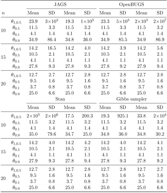
When an improper prior is xed, a lot of care is usually taken in the properness of the posterior distribution. However, the Bayes estimators of log-normal functionals do not exist with the usual priors, both improper and proper (like the inverse gamma). For example, in the context of the log-normal mean, this issue was highlighted by Zellner (1971), and interesting solutions were proposed by Rukhin (1986) and Fabrizi and Trivisano (2012). To provide the general idea of the way in which the non-existence of the posterior moments aects the usual inference based on MCMC methods, a simple simulation exercise is shown as motivating example. Firstly, a random sample from a log-normal distribution with pa-rameters ξ = 2 and σ2 _{= 1} _{is considered as dataset and samples from the posterior of the} target quantities are generated using dierent tools: JAGS through rjags (Plummer, 2016), OpenBUGS (Spiegelhalter et al., 2007), Stan (Carpenter et al., 2017) and implementing the Gibbs samples exploiting the conjugacy of the estimated model, since the conjugate normal-inverse gamma prior is assumed at this stage.

For each method, two independent posterior samples of size1,000,000are generated, after a burn-in period of100,000iterations. The quantities included in the exercise are the sample mean, the median and the quantiles that correspond to p = 0.1 and p = 0.9. All the traceplots of the chains evidenced the convergence to a unique stationary distribution. The mean and standard deviation of the posterior distributions are reported in table 1.1 for three dierent sample sizes n.

Then, the simple one way ANOVA random eect model with J balanced groups having sample sizeng is considered for the response variable logarithm:

log(yij) =µ+νj+εij, i= 1, ..., ng, j= 1, ..., J;

νj ∼ N(0, τ2); εij ∼ N(0, σ2).

(1.9)

In this case, to generate the toy dataset, the parameters are xed as µ = 1, σ2 _{= 1} _and

τ2 _{= 1}_{. Following the indications in Gelman (2006), half-t priors with 3 degrees of freedom} are specied for the scale parameters:

σ∼half−t3,

τ _∼half₋t3.

(15)

JAGS OpenBUGS

n Mean SD Mean SD Mean SD Mean SD

10 θ1,0.5 23.9 3×103 19.3 1×103 23.3 5×103 2×103 2×107 θ0.5 11.5 3.3 11.5 3.2 11.5 3.3 11.5 3.2 θ0.1 4.1 1.4 4.1 1.4 4.1 1.4 4.1 1.4 θ0.9 34.9 86.4 34.8 36.0 34.9 85.5 34.9 86.9 15 θ1,0.5 14.2 16.5 14.2 4.0 14.2 3.9 14.2 5.6 θ0.5 10.5 2.1 10.5 2.1 10.5 2.1 10.5 2.1 θ0.1 4.1 1.1 4.1 1.1 4.1 1.1 4.1 1.1 θ0.9 27.8 9.3 27.8 9.3 27.8 9.2 27.9 9.4 20 θ1,0.5 12.7 2.7 12.7 2.8 12.7 2.8 12.7 2.8 θ0.5 9.5 1.6 9.5 1.6 9.5 1.6 9.5 1.6 θ0.1 3.7 0.8 3.7 0.8 3.7 0.8 3.7 0.8 θ0.9 25.0 6.6 25.0 6.6 25.0 6.6 25.0 6.6

Stan Gibbs sampler

Mean SD Mean SD Mean SD Mean SD

10 θ1,0.5 2×103 2×106 17.5 200.3 19.3 925.1 33.8 2×104 θ0.5 11.5 3.2 11.5 3.2 11.5 3.2 11.5 3.2 θ0.1 4.1 1.4 4.1 1.4 4.1 1.4 4.1 1.4 θ0.9 35.0 79.6 34.7 25.0 34.8 36.0 34.8 30.2 15 θ1,0.5 14.2 4.0 14.2 4.2 14.2 4.0 14.2 4.1 θ0.5 10.5 2.1 10.5 2.1 10.5 2.1 10.5 2.1 θ0.1 4.1 1.1 4.1 1.1 4.1 1.1 4.1 1.1 θ0.9 27.9 9.3 27.8 9.4 27.8 9.3 27.8 9.2 20 θ1,0.5 12.7 2.8 12.7 2.8 12.7 2.8 12.7 2.7 θ0.5 9.5 1.6 9.5 1.6 9.5 1.6 9.5 1.6 θ0.1 3.7 0.8 3.7 0.8 3.7 0.8 3.7 0.8 θ0.9 25.0 6.6 25.0 6.6 25.0 6.6 25.0 6.6

Table 1.1: Results of the MCMC exercise involving the estimation of mean (θ1,0.5), median (θ0.5)

and quantiles (θ0.1,θ0.9) for the toy example.

In this framework, if the goal of the analysis is to predict the group-level mean for the original data scale, the functional considered is:

θc(νl) = exp µ+νj+ σ2 2 , j= 1, ..., J. (1.11)

(16)

to estimate is: θm= exp µ+σ 2₊_τ2 2 . (1.12)

Also in this case, two independent posterior samples are drawn for the target functionals and the posterior means and standard deviations are reported in table 1.2.

JAGS Stan

Mean SD Mean SD Mean SD Mean SD

ng= 3 J = 4 θc(ν1) 8.3 900.1 10.5 2×103 9.3 817.9 785.3 7×105 θc(ν2) 4.3 1×103 14.5 9×103 3.6 308.2 3×104 3×107 θc(ν3) 36.6 329.5 50.0 8×103 39.4 2×103 5×104 5×107 θc(ν4) 9.8 357.1 17.2 6×103 11.5 983.3 2×105 2×108 θm 2×1014 1×1017 1×1023 9×1025 3×10129 2×10132 1×1072 1×1075 ng= 5 J = 4 θc(ν1) 3.8 37.4 3.8 3.4 3.7 3.0 3.8 3.6 θc(ν2) 6.0 20.9 6.0 4.3 6.0 5.1 6.0 4.3 θc(ν3) 21.8 106.9 21.7 32.3 21.6 14.3 21.7 14.8 θc(ν4) 3.4 9.3 3.4 3.2 3.4 2.7 3.3 2.8 θm 3×1028 3×1031 5×108 4×1011 4×1067 4×1070 7×10125 Inf ng= 3 J = 10 θc(ν1) 5.2 2.7 5.2 2.7 5.2 2.7 5.2 2.7 θc(ν5) 3.2 1.9 3.2 1.9 3.2 1.8 3.2 1.8 θc(ν10) 3.2 1.8 3.2 1.8 3.2 1.8 3.2 1.8 θm 7.7 21.3 7.7 9.2 8.1 250.3 7.8 43.9

Table 1.2: Results of the MCMC exercise involving the estimation of global mean (θm) and group

means (θc(νl)) under a one way random eect ANOVA model, considering the toy dataset.

By looking at the tables containing the simulation exercise results, the motivations for the research illustrated in this thesis emerge. Remarking that all the numbers reported in table 1.1 and table 1.2 are, in any way, nite values found estimating a quantity that is not nite under the considered prior settings, the numerical instability of the MCMC estimation outcomes are evident with small sample sizes. This instability manifests itself in two distinct ways: disproportionately large estimates are found for the considered posterior summaries, otherwise dierent values (often apparently reliable) for the same quantity are estimated in dierent runs of the algorithm. Unfortunately, these warnings vanish with the sample size increase and the user is led to believe in the estimates validity.

1.3 Work summary

As hinted before, the issues aecting the Bayesian estimation of the log-normal mean were faced by Fabrizi and Trivisano (2012) and Fabrizi and Trivisano (2016), wherein the log-normal linear model was considered. The core of their proposal consists of specifying a generalized inverse Gaussian (GIG) prior for the variance in the log-scale σ2_{. In this way,}

(17)

existence conditions for the posterior moments of the target functionals to estimate were found and a careful inferential procedure in the Bayesian framework was proposed.

The aim of this work is to ll the gap which is present in the literature approaching the esti-mation of log-normal quantiles (both unconditional and conditional) and of the log-normal linear mixed model form a Bayesian perspective, proposing a mathematically coherent in-ferential procedure.

The thesis is divided into two parts. In the rst one, the quantile estimation problem is faced. In particular, in chapter 2, a new distribution is derived and its properties are reported, and in chapter 3 it is shown that this distribution is crucial in the posterior inference on the target functionalθp and the Bayes estimators are derived; then, in chapter 4, they are rst evaluated in a simulation study and then applied to real data.

The second part about the estimation of the log-normal mixed model is organized with a similar scheme: in chapter 5, the mathematical framework to solve the inferential problem is developed, whereas in chapter 6, a simulation study is carried out and the proposed methods are applied to real data.

Moreover, a particular care to computational aspects was taken in order to facilitate and encourage the practitioners to use the developed methods: an R package named BayesLN is implemented, whose manual is reported in appendix E. It is aimed at enclose functions useful in carrying out a proper Bayesian analysis under the log-normality assumption for data. The methods developed in Fabrizi and Trivisano (2012) and Fabrizi and Trivisano (2016) are implemented in the package too.

(18)

Inference on log-normal quantiles

(19)

The SMNG Distribution

Before addressing the focus on the main topic of this part, that is the Bayesian estimation of log-normal quantiles, some preliminary results are required. The chapter is organized as follows: an introduction to the generalized inverse Gaussian (GIG) distribution is provided in section 2.1, whereas a new family of normal mean-variance mixtures is presented in section 2.2. In section 2.3, the new distribution with the GIG as mixing distribution is derived and its properties are studied, in section 2.4 it is compared to the generalized hyperbolic distribution and its exponential transformation is considered in section 2.5. Finally, some computational details are provided in section 2.6.

2.1 Generalized Inverse Gaussian Distribution

The generalized inverse Gaussian, a general positive real valued distribution, is characterized by the following probability density function:

fX(x) = γ δ λ 1 2Kλ(δγ) xλ−1exp −1₂ δ2 x +γ 2_x , x >0; (2.1) where Kν(x) is the Bessel K function (see appendix A.2). The three parameters (λ, δ, γ) could assume values within the following ranges:

General case: λ_∈R, δ >0, γ >0;

Limiting case I:λ >0, δ→0, γ >0; Limiting case II:λ <0, δ >0, γ→0.

By considering the relation (A.7), it is evident that the rst limiting case corresponds to the gamma distribution, whereas the second one leads to the inverse gamma distribution. Other known distributions might be deduced with particular values of the parameters, like the exponential distribution and the inverse Gaussian distribution (Paolella, 2007).

(20)

On the other hand, the GIG distribution is strictly connected to the positiveα-stable distri-bution. The α-stable distribution represents a very exible 4-parameters distribution that is largely characterized by the so called stability parameterα, whose value controls the tail heaviness. Usually, the density of this family of distributions is not available in closed form and the law is dened in terms of characteristic function. The positiveα-stable distribution is deduced when the skewness parameter assumes the value 1, implying the complete pos-itive skewness. It is possible to prove that the GIG distribution can be obtained starting from the positive α-stable one by applying determined mathematical transforms aimed at obtaining lighter tailed distributions and by considering the caseα = 1/2 (Meyers, 2010). It is possible to considerλas the shape parameter, δ a scale parameter, whereasγ controls the tail heaviness. Figure 2.1 gives an idea of the GIG behaviour with respect to dierent parameter values. In particular, the role of γ is emphasized by plotting the log-density function: it is clear that the lower the value of γ is, the tail of the distribution is heavier. The GIG distribution has all the moments dened for γ > 0, because of its exponential decay in the tail, and they assume the form:

EXj= δ γ j Kλ+j(δγ) Kλ(δγ) . (2.2)

Besides, the moment generating function for the general case is:

MX(r) = γ p γ2₋₂_r !λ Kλ(δ p γ2₋₂_r₎ Kλ(δγ) , r < γ2 2 . (2.3)

Another useful quantity to report in order to characterize the distribution is the mode:

M o(X) = (λ−1) +

p

(λ−1)2₊_δ2_γ2

γ2 ; (2.4)

which is particularly appealing since it is the unique synthetic measure of the GIG distribu-tion that is free of BesselK functions, and hence it is easily tractable. A detailed analysis of the distribution properties could be found in Jorgensen (1982).

2.1.1 The Extended GIG distribution

The power transformation of a GIG random variable is of interest. Let us consider a ran-dom variable X _∼ GIG(λ, δ, γ), then the transformed variable Y = X1θ is distributed as an extended GIG (EGIG) distribution with parameters (λ, δ, γ, θ). The properties of this distribution were studied in Silva et al. (2006): its probability density function can be eas-ily obtained by applying the random variable transformation formula, and the moments immediately follow from the (2.2) withEYj=E

h

Xjθ

i

(21)

0.0 0.5 1.0 1.5 0 5 10 15 x f(x) λ: −1 0 1 0.0 0.1 0.2 0.3 0 5 10 15 x f(x) γ: 1 0.8 0.5 0.0 0.1 0.2 0.3 0 5 10 15 x f(x) δ: 1 3 5 −10.0 −7.5 −5.0 −2.5 0.0 0 5 10 15 x log[f(x)] γ: 1 0.8 0.5

Figure 2.1: Plots of the GIG density function with dierent values of the parametersλ, δandγ. In each plot the other parameters are xed equal to 1. To point out the impact ofγon the tail the log-density is also reported for that parameter.

2.2 Just another normal mean-variance mixture

A widespread and exible family of distributions, which is employed to model data en-dowed with particular features (e.g. multi-modality, heterogeneity, marked skewness and heavy tails) that cannot usually be captured by standard density functions, is the normal mean-variance mixture. The main properties of these distributions were rstly studied in Barndor-Nielsen et al. (1982), but it is still an open research eld (Yu, 2017). A funda-mental paper, that is considered to be the starting point of the idea of mixture distribution, is the one by Barndor-Nielsen (1977), where the author derived the generalized hyperbolic (GH) distribution to model the wind blown sand particle size (see appendix B.1).

In general, the univariate probability distributions belonging to this family are obtained choosing a mixing density g(_·)for the random variableW, that is a non-negative real-valued distribution, and dening the random variable:

X =µ+βW+√W Z, (2.5)

whereµ, β _∈Rare constants. Furthermore, Z is distributed as a standard normal and it is

independent of the mixing variable W. The aim of a random variable dened in this way is to gain exibility in modelling by introducing variability both in the mean and in the variance of a Gaussian distribution.

(22)

From this general denition, it is possible to obtain several mixture distributions by consid-ering dierent mixing distributions. In fact, the GH case cited above is characterized by the assumption thatW is distributed as a GIG. On the other hand, also the normality assump-tion, executed by setting Z ∼ N(0,1), might be relaxed employing other distributions like the skew normal (Arslan, 2015).

In this section, a new family of distributions strictly related to the normal mean-variance mixture is introduced. It could be named scale-mean mixture of normal distribution and, to my knowledge, it has not received any attention in the literature.

Denition 2.1. Considering two independent distributions Z _{∼ N}(0,1) and W _∼ g(_·), non-negative real valued random variable, then the distribution dened as:

X =µ+β√W +√W Z, (2.6)

µ, β _∈R, is a scale-mean mixture of normal distribution.

A random variable dened in this way, has the following conditional distribution: X_|W =w_{∼ N} µ+β√w, w

; (2.7)

and it is similar to the standard Gaussian mean-variance mixture, since it simply introduces a lower degree of variability in the mean. In fact, the term √W appear in the (2.7) instead of W, which characterizes the usual normal mean-variance mixture.

2.3 A new mixture with GIG as mixing distribution

In this section, the scale-mean mixture of normal distribution is considered in the case W ∼GIG. A parallel result to the one related to the GH distribution is deduced and the derived distribution is labelled as SMNG, which synthesizes a Scale-Mean mixture of Normal distribution assuming a GIG distribution on the scale.

Theorem 2.1 (SMNG Distribution). Let consider the following scale-mean mixture of nor-mal distribution:

X_|W =w_{∼ N} µ+β√w, w

, W _∼GIG(λ, δ, γ); (2.8)

then the random variable X marginally assumes a SMNG distribution with parameters

(λ, δ, γ, µ, β), under the conditions δ, γ > 0. Besides, the probability density function of

X can be expressed: (i) in integral form:

fX(x) =c(λ, δ, γ, β) Z ∞ 0 t−2λexp −1 2 [(x−µ)2+δ2]t2+ +γ 2 t2 −2β(x−µ)t dt; (2.9)

(23)

(ii) as an innite sum: fX(x) =c(λ, δ, γ, β) +∞ X i=0 [β(x₋µ)]i i! Kλ−i+1 2 γpδ2_{+ (}_x₋_µ₎2_× γ p δ2_{+ (}_x₋_µ₎2 !λ−i+1₂ ; (2.10) where: c(λ, δ, γ, β) = γ δ λ √ 2πKλ(δγ)e −β2 2 . (2.11)

Proof. (i) To nd the marginal density function of X, the following integral needs to be solved: fX(x) = Z ∞ 0 fN(x|w)fGIG(w)dw = γ δ λ 2√2πKλ(δγ) Z ∞ 0 wλ−12−1exp −1₂ (x₋µ₋β√w)2 w + +δ 2 w +γ 2_w dw. (2.12)

By using simple algebra it can be noted that: (x−µ−β√w)2 w = (x−µ)2 w − 2β(x−µ) √ w +β 2_. _(2.13)

If this expression is plugged into the integral and the change of variablew=t−2 _{is performed} (dw=₋2t−3_d_t_{), the result of equation (2.9) is deduced.}

(ii) To obtain the innite sum, it is required to recognize that the integral in (2.9) is the kernel of the Laplace transformation of the EGIG density function with parameters

−λ+1₂,pδ2_{+ (}_x₋_µ₎2_{, γ,}₂, whose moments are known (see section 2.1.1) and can be used as follow: fX(x) = γ δ λ e−β 2 2 √ 2πKλ(δγ) K₋_λ+1 2(γ p δ2_{+ (}_x₋_µ₎2₎ (p δ2_{+ (}_x₋_µ₎2_/γ₎−λ+1₂ Z ∞ 0 ertfEGIG(t)dt, (2.14) wherer=β(x−µ).

To complete the proof and get the (2.10) it is necessary to expand the exponential inside the integral. Since the series and the integral are bounded, the summation and the integral can be exchanged: Z ∞ 0 ertfEGIG(t)dt= +∞ X i=0 ri i! Z ∞ 0 tifEGIG(t)dt. (2.15)

(24)

It is possible to recognize that the obtained integrals inside the sum are the moments of order iof the EGIG distribution. By substituting their expressions the nal result is obtained. Unfortunately, it is not possible to obtain a representation of the SMNG density function without an integral or an innite sum. In fact, the integral in (2.9) cannot be expressed in term of known special functions and it is not possible to apply the formula (A.10), i.e. the multiplication theorem of the Bessel K function to the innite sum in (2.10) because of the fractional index in the order.

Even if the convergence of the series (2.10) is a consequence of the equivalence with the convergent integral (2.9), it is also possible to prove it analytically. In fact, considering the standard ratio test, the equivalence (A.5) and the approximation (A.8), the generic term of the sum with j_→+_∞ and ν=₋λ+j+1₂ is:

aj = [β(x₋µ)]j j! r 2 π e δ2_{+ (}_x₋_µ₎2 2 !ν ν−ν−12. (2.16) Consequently, the ratio test assumes the form:

aj+1 aj → 1 j q j 2 + 1−λ −λ+ j+1₂ −λ+₂j + 1 !j₂+1−λ = 0, j_→+_∞, (2.17) and the series is absolutely convergent.

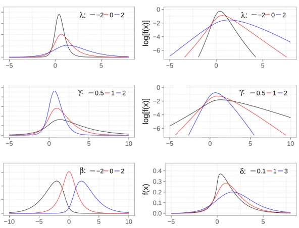
2.3.1 Meaning of the parameters

The inuence of the ve parameters is really similar to the ones of the GH distribution. Figure 2.1 is aimed at giving an idea of the implications that dierent parameters values have on the SMNG density function. The parameterµ operates on location and it induces a shift for the density. Then, it is possible to say that γ inherits its role in the GIG distribution and it is a shape parameter: smaller values imply heavier tails, as it is possible to see observing the log-density plots. Its strict connection to the tail heaviness is also evident from its involvement in the moment generating function existence condition, as will be investigated in the following sections. Another parameter that inuences the tails is λ. On the other hand, β is an asymmetry parameter, whereas δ is the scale parameter: with smaller values the distribution is more concentrated around the peak.

Another useful result about the parameters is the behaviour of the SMNG distribution with respect to changes in location and scale.

Proposition 2.1 (Location-scale behaviour). IfX∼SM N G(λ, δ, γ, µ, β)and two constant

a_∈R\ {0}, b∈R are considered, then:

aX +b∼SM N G λ,|a|δ, γ |a_|, β, aµ+b . (2.18)

(25)

Proof. To prove this result, it is sucient to obtain the density function of the transformed random variable: faX+b(x) =a−1fX x₋b a ;λ, δ, γ, β, µ . (2.19)

After simple algebra and a change of variable into the integral, it is possible to get:

faX+b(x) = γ a2_δ λ √ 2πKλ(aδa−1γ) e−β 2 2 Z ∞ 0 z−2λ_× ×exp −1₂ (x₋b₋aµ)2+a2δ2 z2+ γ 2 a2_z2+ −2β(x₋b₋aµ)z dz (2.20) Fixing _δ˜ ₌ _|_a_|_δ_, _˜_γ ₌ γ

|a| and µ˜ = aµ+b and comparing the previous density in (2.9)

it is clear that it is again the density function of a SMNG distribution with parameters

λ,˜δ,˜γ, β,µ˜.

2.3.2 Moment generating function and moments of the distribution The general results that can be obtained for the conventional cases of normal mean-variance mixtures (Hammerstein, 2010) do not hold for the SMNG distribution because of the par-ticular form of the density function. Therefore, it is necessary to algebraically deduce the quantities that characterize the distribution, beginning from the moment generating func-tion.

Theorem 2.2 (SMNG Moment Generating Function). Considering a random variableX∼ SM N G(λ, δ, γ, µ, β), it has a moment generating function of the form:

MX(r) =eµr γ √ γ2₋_r2 λ Kλ(δγ) +∞ X i=0 (rβ)i i! δ p γ2₋_r2 !₂i K_λ+i 2 δpγ2₋_r2_, (2.21) that is dened if r < γ.

Proof. To get simpler computations, the case µ = 0 is considered. Recalling the integral form of the density function (2.9), using the denition of moment generating function:

MX(r) = γ δ λ √ 2πKλ(δγ) e−β 2 2 Z +∞ −∞ erx Z ∞ 0 t−2λ× ×exp −1 2 [x2₊_δ2_]_t2₊γ2 t2 −2βxt dtdx. (2.22)

(26)

0.0 0.2 0.4 0.6 0.8 −5 0 5 f(x) λ: −2 0 2 0.0 0.1 0.2 0.3 0.4 0.5 −5 0 5 10 f(x) γ: 0.5 1 2 0.0 0.1 0.2 0.3 −10 −5 0 5 10 x f(x) β: −2 0 2 −6 −4 −2 0 −5 0 5 log[f(x)] λ: −2 0 2 −6 −4 −2 0 −5 0 5 10 log[f(x)] γ: 0.5 1 2 0.0 0.1 0.2 0.3 0.4 −5 0 5 x f(x) δ: 0.1 1 3

Figure 2.2: Comparison of the SMNG density with dierent values of the parameters. In the legend the varying parameters are showed, the other are xed equal to1with the exception ofµ= 0. For

λandγalso the logarithm of the density is reported.

By applying Fubini's theorem and after a change of variable it is possible to recognize the integral of the Gaussian distribution moment generating function. It can be solved using the formula 3.323.2 in Gradshteyn and Ryzhik (2014):

MX(r) = γ δ λ √ 2πKλ(δγ)e −β₂2 Z ∞ 0 t−2λ−1_exp −1 2 δ2_t2₊ γ2 t2 × × Z +∞ −∞ exp −z 2 2 + z(r+βt) t dzdt= = γ δ λ Kλ(δγ) Z ∞ 0 t−2λ−1exp −1₂ δ2t2+γ 2₋_r2 t2 − 2rβ t dt. (2.23)

The latter integral is convergent ifr < γand, through another change of variable, an integral with the same structure as the one in (2.14) is obtained. Therefore, if the same procedure used to prove the statement (ii) of Theorem 2.1 is applied, the (2.21) can be deduced (up to the term eµr_).

(27)

Finally, the result can be extended to anyµby applying Proposition 2.1 and the formula of the moment generating function of a linearly transformed random variable. In order to derive a generic expression for the SMNG distribution moments, it is useful to start from the particular case µ= 0.

Proposition 2.2 (SMNGj-th Moment). IfZ _∼SM N G(λ, δ, γ, β,0), then thej-th moment assumes the following form:

EZj=      2_γδ j 2 Kλ+j₂(δγ) Kλ(δγ) Γ(j+1₂ ) √ π Φ −2j, 1 2;− β2 2 j even β2δ γ j₂ K_λ₊j 2 (δγ) Kλ(δγ) √ 2Γ(₂j+1) √ π Φ 1−j 2 , 3 2;− β2 2 j odd (2.24)

where Φ(_·,_·;_·) is the Kummer's M conuent hypergeometric function (see appendix A.3). Proof. Thej-th moment of Z is dened as:

EZj= γ δ λ √ 2πKλ(δγ) Z +∞ −∞ zp Z +∞ 0 t−2λ_exp −1 2 (zt₋β)2₊ +γ 2 t2 +δ 2_t2 dxdt= (2.25) = γ δ λ √ 2πKλ(δγ) Z +∞ 0 t−2λ_exp −1 2 γ2 t2 +δ 2_t2 × × Z +∞ −∞ zj_exp −1 2 (zt₋β)2 dz dt; (2.26)

by Fubini's theorem. With the substitution zt=y, in the inner integral the j moment of a N(β,1)can be recognized.

Recalling that thej-th moment of a Gaussian distribution with meanµ and varianceσ2 _is dened as (Winkelbauer, 2012): E[Yj] = (iσ)jexp −µ 2 4σ2 Dj −iµ σ , (2.27)

whereDν(x)is the Parabolic Cylinder function (see appendix A.4), then applying the inte-gral representation (A.4) to the (2.26) it is obtained:

EZj= δ γ j 2 K_λ+j 2 (δγ) Kλ(δγ) (i)jexp −β 2 4 Dj(−iβ). (2.28) By using the expression ofDν(x) as a function of the Kummer'sM function (A.15) and by applying the Euler reection formula (A.2) to the gamma functions the nal form (2.24) is

(28)

Then, if a generic SMNG distribution is considered, through Proposition 2.2 it is possible to get an expression for the moments of the formE(X−µ)j. However, the following lemma

gives the possibility to use this particular result in order to compute both the raw moments

EXjand the central moments E h

(X−E[X])j i

of any SMNG distribution. Lemma 2.1. For any constant aand b and any positive integer j, it is true that:

E(X−b)j= j X l=0 j l (a−b)j−lE h (X−a)li. (2.29)

Proof. See Scott et al. (2011).

After the general denition of the moments and of the moment generating function, the characterization of the distribution can be completed writing the expected value:

E[X] =µ+β δ γ 1₂ K λ+1 2(δγ) Kλ(δγ) ; (2.30)

and the variance:

V[X] =β2 δ γ   Kλ+1(δγ) Kλ(δγ) − K2 λ+1₂(δγ) K2 λ(δγ)  + + δ γ Kλ−1(δγ) +Kλ+1(δγ) 2Kλ(δγ) − λ γ2. (2.31)

These expressions could be deduced by applying theE[·]andV[·]operators to the formulation

in (2.6) or through the moment generating function. 2.3.3 Particular cases

Since the GIG distribution includes two important limiting cases, which coincide with the inverse gamma and the gamma distributions, it is interesting to explore the resultant mixture distributions.

Inverse Gamma as mixing distribution

If the GIG distribution hasλ <0andγ _→0, then the random variable is an inverse gamma

W ∼IG(α, θ): fW(w) = θα Γ(α)w −α−1_e−θw−1 , w >0. (2.32)

In this case, the integral (2.9) simplies and it is possible to recognize the integral form of the parabolic cylinder function (A.14). Therefore, the marginal density function of the

(29)

SMNG reduces to: fX(x) = θα_{Γ (2}_α_{+ 1)}_D −2α−1 β(µ−x) √ (x−µ)2_+2θ √ 2πΓ(α) [(x₋µ)2_{+ 2}_θ_]α+1₂ × ×exp β2₍_µ₋_x₎2 4 [(x₋µ)2_{+ 2}_θ_]− β2 2 , (2.33) whereθ= δ2

2 and α=−λif the parametrization of (2.8) is considered.

In agreement with the existence condition of the SMNG moment generating function (see theorem 2.2), it turns out that in this particular case MX(r) is not dened.

Gamma as mixing distribution

If the limiting case I of the GIG distribution is examined, i.e. λ >0andδ _→0, the gamma distribution of parametersλand ν = γ₂2 is the mixing distribution and the density ofX is:

fX(x) = √ 2νλ √ πΓ(λ)e −β2 2 +∞ X i=0 [β(x−µ)]i i! Kλ−i+1 2 √ 2ν|x−µ|× √ 2ν |x₋µ_| !λ−i+1 2 . (2.34)

It has the same structure of the (2.10) and the existence conditions of the moment generating functions remain the same as in the general case.

2.4 Comparison with the GH distribution

The distribution considered in Theorem 2.1 denes a real-valued random variable that has a similar behaviour with respect to the GH distribution. First of all, if it is xed β = 0 the SMNG distribution assumes the same limiting case of the GH, i.e. the symmetric GH distribution.

Since the two distributions depend on 5 parameters that have the same meaning, it is interesting to observe the changes in the densities taking equal parameters sets. In gure 2.3, the main dierence between the two distributions clearly appears: the right tail (left in case of negativeβ) is considerably lighter for the SMNG distribution.

In eect, the density of a GH distribution in the tails is: fGH(x) =c|x|λ−1exp

n

−pγ2₊_β2_|_x_|₊_βxo_, _|_x_{| → ∞} _(2.35) that denes a distribution with semi-heavy tails; whereas the tails of the SMNG distribution, recalling the (A.9), have the following law:

fSM N G(x) =c_|x_|λ−1expn₋γ_|x_|+√γβ_|x_|12

o

(30)

0.0 0.1 0.2 0.3 −5 0 5 10 15 x f(x) β=1 SMNG GH 0.00 0.05 0.10 0.15 0.20 0.25 −5 0 5 10 15 x f(x) β=3 SMNG GH −6 −4 −2 0 −5 0 5 10 15 x log[f(x)] β=1 SMNG GH −10.0 −7.5 −5.0 −2.5 0.0 −5 0 5 10 15 x log[f(x)] β=3 SMNG GH

Figure 2.3: Plots of GH and SMNG densities and log-densities with the same parameters xed: the casesβ = 1andβ = 3are reported. The other parameters are xed equal to1 with the exception

ofµ= 0.

Therefore, for each β >0and it is possible to conclude that:

fGH(x0)> fSM N G(x0), ∀x0 > M, (2.37) where M is a large positive number. The same holds for the left tail with β < 0 and M negative. On the other hand, if the left tail with β >0 is considered, then the GH density decays faster than the SMNG density.

2.5 The log-SMNG distribution

In the subsequent parts of this work, the distribution of the exponential transformation of a SMNG distributed random variable is of interest. This kind of distribution can be dened as follow.

Denition 2.2 (Log-SMNG distribution). If X _∼ SM N G(λ, δ, γ, β, µ), then the random variable Y = exp_{X_} assumes a log-SMNG distribution. Equivalently, the log-SMNG tribution might be dened as the random variable whose logarithmic transformation is dis-tributed as a SMNG.

(31)

Therefore, a continuous distribution that assumes positive values only is faced. With a simple application of the random variable transformation formula, it is possible to deduce the key properties that characterize the distribution.

Proposition 2.3 (Log-SMNG characterization). If X _∼ SM N G(λ, δ, γ, β, µ) and Y = exp_{X_}, then Y possesses:

(i) probability density function:

fY(y) = 1

yfX(log[y]), (2.38)

where fX(·) is dened in the (2.9) or (2.10);

(ii) expectation and j-th central moment (dened if γ > j):

E[Y] =eµ γ √ γ2₋₁ λ Kλ(δγ) +∞ X i=0 (β)i i! δ p γ2₋₁ !₂i K_λ+i 2 δpγ2₋₁_, (2.39) E[Yj] =ejµ γ √ γ2₋_j2 λ Kλ(δγ) +∞ X i=0 (jβ)i i! δ p γ2₋_j2 !₂i K_λ+i 2 δpγ2₋_j2_. _(2.40)

Proof. (i) The result follows from the simple application of the random variable transfor-mation formula.

(ii) Given that Y = exp{X}, then E[Yj] = E[exp{jX}]. It is the moment generating

function of the SMNG distribution dened in the (2.21) evaluated in j. Consequently, the existence of the moments of the log-SMNG is regulated by the same existence condition of

the SMNG moment generating function.

2.6 Computational notes and software implementation

In order to use the two distributions described in this chapter, R (R Core Team, 2017) functions needed to be implemented. In particular, to generate random samples from the SMNG distribution, the mixture specication in (2.8) was exploited. Therefore, to obtain an independent sample of sizen the following steps were executed:

generate a sample of n independent realizations from a GIG distribution using the function rgig(), included in the R package ghyp (Breymann and Lüthi, 2013); use rnorm() to generate from the resultant normal distribution.

Another function implements the SMNG density function. This is a tricky task because of the numerical instability of the two formulations given in Theorem 2.1. In fact, with high

(32)

values of the parametersδ, γ, β, numerical problems might be detected both for the function based on integrate() and the innite sum, that includes a ratio of Bessel K functions. To overcome this issue, the best solution is to implement the sum in (2.10) with the option expon.scaled=TRUE of the function besselK(), that returns exp{x}Kν(x). In this way, the eventual problems related to the numerical underow caused by the ratio of two Bessel K functions with elevate arguments can be avoided. Besides, an easy way to implement a stopping rule for the innite sum consists in putting a test in order to evaluate the magnitude of each term with respect to the partial sum. However, a function that produces the density through the integral representation was implemented too.

Then, to get the cumulative distribution function: FX(x) =

Z x

−∞

fX(t)dt, (2.41)

a numerical integration procedure was employed through the integrate() function. Finally, the computation of the quantiles represents a famous problem of numerical inversion. In fact, the quantile α that corresponds to a probability p is the solution of the non-linear equation:

FX(α)−p= 0. (2.42)

To solve it, the standard uniroot() procedure was employed (Lange, 2010).

The same ideas were used to implement the key functions related to the log-SMNG distri-bution, by applying the simple exponential transformation to the generated sample and the formula (2.38) for the density.

All these functions are implemented in R and included in the developed package BayesLN. The standard R denominations are adopted: dSMNG and dlSMNG evaluate the SMNG and the log-SMNG density functions, pSMNG and plSMNG the cumulative functions, qSMNG and qlSMNG the quantiles and, nally, rSMNG and rlSMNG allow to generate random numbers form the distributions. Moreover, the SMNG moments are implemented in the function SMNGmoment, whereas the function that evaluates the moment generating function is SMNG_MGF.

(33)

Bayesian inference for the log-normal

quantiles

The estimation of log-normal quantiles can be of interest in many applications. For example, in environmental monitoring and occupational health analyses, it is common to estimate extreme quantiles in the right tail of a skewed distribution from small samples (Bullock and Ignacio, 2006; Gibbons et al., 2009; Krishnamoorthy et al., 2011), or to compare a xed legal exposure limit to an extreme quantile (or to its upper condence limit, UCL) estimated from a sample that could be small. Under these conditions, the tools available in the current literature, that mainly consist of the exponentiation of standard frequentist results obtained in the log-scale, can produce unecient point and interval estimators with poor coverage or low precision and can be signicantly improved. The proposed methodology improves current methods, especially in the analysis of small samples. The estimation of quantiles is relevant in several other applied elds like the analysis of lifetime data (Lawless, 2003) or ood frequency analysis (Stedinger, 1980; Hamed and Rao, 1999).

The estimation of log-normal quantiles has received little attention so far. In the frequentist literature, Longford (2012) identies a class of estimators depending on two constants that he determines with the aim of minimizing the frequentist mean square error (MSE); he overlooks relevant inferential problems such as interval estimation.

In this chapter the problem of Bayesian estimation of log-normal quantile is studied with a particular focus on the posterior moment niteness. In section 3.1 an overview on the already developed methods for the log-normal quantile estimation is provided. All the mathematical details to obtain a rigorous Bayesian inferential framework are presented in section 3.2, while in section 3.3 the hyperparameter specication strategy is discussed. Finally, the methodology is extended to the conditional quantile estimation problem in section 3.4.

(34)

3.1 Estimation of log-normal quantiles: current state of the

art

3.1.1 Non-parametric estimation

A non-parametric approach for the quantile estimation is often adopted. Even if the cor-nerstone on this work is the log-normality distributional assumption, it is worth to consider this estimation procedure that is commonly used also with small sample sizes.

There exist a lot of dierent methods easily accessible in common statistical software and a good review is the paper by Hyndman and Fan (1996). As a benchmark for the developed proposals, the standard R function quantile is used, with the default type 7 method. It is due to Gumbel (1939) and it is based on the empirical cumulative distribution function built on the following denition ofk-th plotting position:

pk =

k₋1

n−1, (3.1)

that coincides with the mode of the distribution function of thek-th order statistic: F(X_(k)). Then, the quantile p, included between the positions k−1 and k, is obtained by linear interpolation: ˆ Q7_p =X_(k−1)− X(k−1)−X(k) pk+1−p pk+1−pk . (3.2) 3.1.2 Naive estimation

When an estimate of the log-normalp-th quantile is required, the usual procedure is to take the exponential of the well known normal quantile formula:

ˆ

θp = exp

n

ˆ

ξ+ Φ−1(p)ˆσo, (3.3)

plugging the unbiased estimates of the mean and variance in the log-scale: _ξ,ˆ_σ_ˆ2_{. It is worth} to highlight that, after the squared root transformation,σˆis not an unbiased estimator of the population standard deviation in the log-scale. Besides, even if a monotone transformation (as the exponential is) does not change the order statistics like the quantiles, it might aect all the desirable properties that the estimator has in the original scale.

The same procedure is applied to compute the extremes of the condence intervals (Gibbons et al., 2009). In the two sided case with the xed condence level1₋α they are:

exp ˆ ξ+t₍α 2,n−1,kp) ˆ σ √ n ; exp ˆ ξ+t₍₁₋α 2,n−1,kp) ˆ σ √ n , (3.4) wheret₍α 2,n−1,kp)is the quantile α

2 of a non-central Student's t distribution withn−1degrees of freedom and a non-centrality parameter kp =√nΦ−1(p).

(35)

In many applications, the one-sided intervals are particularly useful, and they are called lower condence limit (LCL) or upper condence limit (UCL):

LCLp = exp ˆ ξ+t(α,n−1,kp) ˆ σ √ n , U CLp = exp ˆ ξ+t(1−α,n−1,kp) ˆ σ √ n . (3.5)

3.1.3 Longford's minimum MSE estimator

In the paper by Longford (2012), the following statistic was proposed to estimate the quan-tilesθp of a sample of observations assumed log-normally distributed:

Qp = exp n ˆ ξ+bpσˆ+dpσˆ2 o , (3.6)

where_ξˆ_and _σ_ˆ2 _{are the unbiased estimators of}_ξ _and_σ2_.

The values of the parameters (bp, dp) were xed by minimizing the MSE of the estima-tor using the Newton-Raphson algorithm. The procedure was implemented by the author substituting the sample quantityσˆ2 _{to the unknown} _σ2_.

It is important to point out that the proposed estimator has nite expectation when dp is negative or when:

σ2 < n−1

2dp

, (3.7)

where n is the sample size. The same inequality divided by 2 determines the existence condition for the MSE. These conditions are not testable since the varianceσ2 _{is not known.}

3.2 Bayes estimator of the log-normal quantiles

The goal is to make inference on the log-normal quantiles θp dened in the (1.5) from the observed sample of sizen: (y1, . . . , yn). The logarithmic transformations of the observations arewi= log(yi).

Therefore, in order to obtain the posterior distribution of θp, it is necessary to assume a prior distribution for the two parametersξandσ2_{. The conjugate Normal-GIG (NGIG) prior} distribution is chosen (Thabane and Haq, 1999). Therefore, a normal prior conditionally on σ2 _{is assumed for} _ξ _{and a generalized inverse Gaussian distribution is specied for} _σ2_:

ξ_|σ2_{∼ N} ξ0, σ2 n0 , (3.8) σ2 _∼GIG(λ, δ, γ). (3.9)

Through the specication of the set of hyperparameters (ξ0, n0, λ, δ, γ) it is possible to ex-press a huge amount of dierent prior situations. It is worth to highlight the fact that the

(36)

marginal prior assumed onξ is a symmetric generalized hyperbolic distribution (see section B.1).

The usual non-informative improper priors like Jerey's prior, are not considered in this case because a key point of the work is to obtain a posterior distribution with nite moments, in order to deduce a Bayes estimator for the estimand, as it will be pointed out later.

Furthermore, to x the notation, from now on the target functional in the log-scale will be dened as:

ηp= logθp

=ξ+ Φ−1(p)σ; (3.10)

and the following sample quantities will be employed: ¯ w= Pn i=1wi n ; (3.11) v2 ₌ Pn i=1(wi−w¯)2 n . (3.12)

Before deducing the posterior distribution of θp, a series of useful results conditioned on σ2 could be stated. They easily follow from the conjugacy of the NGIG prior with the Normal distribution.

Proposition 3.1. If the Normal prior on ξ (3.8) is specied and the log-normal model is assumed for data, then the following results conditioned on σ2 _hold:

(i) ξ_|σ2,w_{∼ N} ξ1, σ2 n1 , (3.13) where ξ1 =ψw¯+ (1−ψ)ξ0,n1 =n+n0 andψ= _n1n; (ii) ηp|σ2,w∼ N ¯ ηp, σ2 n1 , (3.14) where η¯p =ξ1+ Φ−1(p)σ. Proof. (i) It is necessary to consider:

p(ξ_|σ2,w)_∝p(w_|ξ, σ2)p(ξ, σ2) ∝exp ( − Pn i=1(wi−ξ) 2 2σ2 − n0(ξ−ξ0)2 2σ2 ) = exp ( − Pn i=1(wi−w¯) 2 2σ2 − n1(ψw¯+ (1−ψ)ξ0−ξ)2 2σ2 ) ∝exp ( −n1(ξ1−ξ) 2 2σ2 ) ; (3.15)

(37)

that is the kernel of a Gaussian distribution with mean ξ1 and variance σ 2 n1.

(ii) To prove this point it is possible to observe from (3.10) that ηp is a simple linear transformation ofξ and the same transformation can be applied to the normal distribution.

As a direct consequence of the previous proposition, the target functional θp assumes a log-normal distribution conditionally on σ2_.

Another important step is the derivation of the marginal posterior distributions for the parametersξ andσ2_{. Also in this case a standard result is faced, because of the conjugacy} of the Normal prior on the Gaussian mean.

Proposition 3.2. If the NGIG prior (3.8), (3.9) is specied and the log-normal model is assumed for data, then the posterior marginal distributions for the parametersξ andσ2 _are:

(i) ξ|w∼GH λ,¯ ¯γ,0,δ, ξ¯ 1 , (3.16) where ¯_λ₌_λ₋n 2, ¯γ = √_n 1γ andδ¯= √n1 −1√ δ2₊_nv2. (ii) σ2_|w_∼GIG λ,¯ δ¯√n1, γ . (3.17)

Proof. (i) Integrating outσ2 _{from the joint distribution and then applying (A.4):}

p(ξ_|w)_∝ Z +∞ 0 p(w_|ξ, σ2)p(ξ, σ2)dσ2 ∝ Z +∞ 0 (σ2)−n+12 exp − 1 2σ2 nv2+n1(ψw¯+ (1−ψ)ξ0−ξ)2 × × σ2λ−1 exp −1₂ δ2 σ2 +γ 2_σ2 dσ2 = Z +∞ 0 (σ2)λ−n+12 −1exp −1₂ δ2₊_nv2₊_n 1(ξ−ξ1)2 σ2 +γ 2_σ2 dσ2 ∝ Kλ− n+1 2 γpδ2₊_nv2₊_n₁₍_ξ₋_ξ₁₎2 _p δ2₊_nv2₊_n₁₍_ξ₋_ξ₁₎2_/γ n+1 2 −λ . (3.18)

The obtained expression is the kernel of a symmetric GH distribution (i.e. β= 0). (ii) Starting from the same point of part (i) but integrating out ξ:

p σ2_|_w ∝ Z +∞ −∞ p(w_|ξ, σ2₎_p₍_{ξ, σ}2_)d_ξ ∝(σ2)λ−n+12 −1exp −1₂ δ2 σ2 +γ 2_σ2 × Z +∞ −∞ exp − 1 2σ2 n1(ψw¯+ (1−ψ)ξ0−ξ)2 dξ. (3.19)

(38)

The integral is trivial since the kernel of a Gaussian distribution can be noted. Finally, the

kernel of a GIG distribution can be recognized.

The main result of this section consists in the statement of the posterior distribution forθp. Theorem 3.1. If the NGIG prior (3.8), (3.9) is specied and the log-normal model is assumed for data, then:

(i)

ηp|w∼SM N G(¯λ,δ,¯ γ,¯ β, ξ¯ 1), (3.20) where _β¯₌√_n_1Φ−1₍_p₎_;

(ii)

θp|w∼logSM N G(¯λ,¯δ,¯γ,β, ξ¯ 1). (3.21) Proof. (i) Recalling the conditional distribution ofηpwith respect toσ2 (3.13), the quantity could be written as:

1 √_n 1 ηp|σ2,w∼ N √n1ξ1+√n1Φ−1(p)σ, σ2 . (3.22)

Since from the (3.17) it is known that the posterior distribution of σ2 _{is GIG, the result of} Theorem 2.1 can be used to obtain:

1 √_n 1 ηp|w∼SM N G(¯λ, p δ2₊_n 1v2, γ,β,¯ √n1ξ1). (3.23) To complete the proof, it is required to apply the result on the location-scale behaviour of the SMNG distribution studied in proposition 2.1.

(ii) Sinceηp|wis SMNG distributed andθp = exp{ηp}, then by denition 2.2 it is log-SMNG

distributed.

The deduced parameters of the θp posterior distribution are compliant with the meaning of the SMNG parameters: a higher posterior sample size n1 implies lighter tails (smaller and negative λand bigger γ) and a density that is gathered around the mode (smaller δ). On the other hand, the asymmetry parameter β is ruled by the studied quantile through the inverse of the standardized Gaussian cumulative distribution function, and the location parameter is equal to the conditioned posterior meanξ1.

As already shown in section 2.5, it is possible to deduce the moments of the log-SMNG distribution by starting from the moment generating function of the SMNG distribution. Since one of the aims of this work is to get a point estimate of the target quantity (Lehmann and Casella, 2006; Robert, 2007), the Bayes estimator associated to a given loss function, according to denition C.2, is investigated and evaluated. To have a brief introduction to Bayesian point estimation under loss functions see section C.

This kind of estimators represents a convenient way to synthesize the posterior distribution. In particular, the quadratic loss function (C.4) is considered in this work for its popularity

(39)

and the relative quadratic loss function (C.6) is included too because of its history in the context of Bayesian log-normal estimation. This aspect will be deepened in the following sections. The Bayes estimators associated to the considered loss functions respectively are the posterior mean and the ratio of posterior expectations reported in equation (C.7). Proposition 3.3 (Bayes estimators of θp). Given that the posterior distribution for the target functional θp is (3.21), then:

(i) the Bayes estimator of the log-normal p-th quantile under the quadratic loss function is: ˆ θQB p =eξ1 √ n1γ √ n1γ2₋₁ λ¯ K¯_λ( √ nv2₊_δ2_γ₎ +∞ X j=0 ¯ βj j! √ nv2₊_δ2 √_n 1 p n1γ2−1 !j₂ × ×K_λ+¯ j 2 √ nv2₊_δ2p n1γ2−1 √_n 1 ! , (3.24)

that exists when γ > √1

n;

(ii) the Bayes estimator under relative quadratic loss is:

ˆ θ_pRQB =eξ1 p n1γ2−4 p n1γ2−1 !λ¯ × × P+∞ j=0 ¯ βj j! _√ nv2_+δ2 √ n1√n1γ2₋₁ j 2 K_λ+¯ j 2 √ nv2_+δ2√_n1_γ2₋₁ √ n1 P+∞ j=0 ¯ βj j! 4√nv2_+δ2 √ n1√n1γ2₋₄ ₂j K_λ+¯ j 2 √ nv2_+δ2√_n1_γ2₋₄ √ n1 ; (3.25)

that exists when γ > √2

n1.

Besides, to have a nite posterior variance it must hold that: γ > _√2

n1

. (3.26)

Proof. (i) Since the Bayes estimator under quadratic loss is the posterior mean, consider-ing that θp|w follows a log-SMNG distribution, the result is a simple application of the proposition 2.3.

(ii) To get the Bayes estimator under relative quadratic loss it is sucient to note that by applying proposition 2.1:

−log(θp)|w∼SM N G(¯λ,δ,¯ γ,¯ β,¯ −ξ1), (3.27) −2 log(θp)|w∼SM N G(¯λ,2¯δ,γ/¯ 2,β,¯ −2ξ1); (3.28) and then it is required to use proposition 2.3 to get an expression for (C.7).