The Performance (and Limits) of Simple Neuron Models: Generalizations of the Leaky Integrate-and-Fire Model

Models: Generalizations of the Leaky

Integrate-and-Fire Model

Richard Naud and Wulfram Gerstner

The study of neuronal populations with respect to coding, computation and learning relies on a primary building bloc: the single neuron. Attempts to understand the essence of single neurons yield mathematical models of various complexity. On one hand there are the complex biophysical models and on the other hand there are the simpler integrate-and-fire models. In order to relate with higher functionalities such as computation or coding, it is not necessary to model all the spatio-temporal details of ionic flow and protein interactions. There is a level of description that is simple, that bridges the gap to higher functionalities, and that is sufficiently complete to match real neurons. In this chapter we start with the integrate-and-fire model and then consider a set of enhancements so as to approach the behaviour of multiple types of neurons.

The formalism considered here takes a stimulating currentI(t)as an input and responds with a voltage traceV(t), which contain multiple spikes. The input cur-rent can be injected experimentallyin vitro. In a living brain, the input comes from synapses, gap junctions or voltage-dependent ion channels of the neuron’s mem-brane.I(t)in this case corresponds to the sum of currents arriving to the compart-ment responsible for spike generation.

1 Basic Threshold Models

Nerve cells communicate by action potentials – also called spikes. Each neuron gathers input from thousands of synapses to decide when to produce a spike. Most

Richard Naud

Ecole Polytechnique F´ed´erale de Lausanne, Lausanne, 1015-EPFL, Switzerland, e-mail: [email protected]

Wulfram Gerstner

Ecole Polytechnique F´ed´erale de Lausanne, Lausanne, 1015-EPFL, Switzerland, e-mail: [email protected]

I(t)

+

-+

+

+

+

--

-g

E

C

V

Fig. 1 Positively and negatively charged ions are distributed inside and outside the cell. Current (I(t)) entering the cell will modify the difference in electric potential between the exterior and the interior (V). The dynamics of the LIF correspond to a RC-circuit composed of a conductance (gL) in parallel with a capacitance (C). The electric supply corresponds to the resting potential (EL).

neurons will fire a spike when their membrane potential reaches a value around -55 to -50 mV. Action potential firing can be considered an all-or-nothing event. These action potentials are very stereotypical. This suggests that spikes can be replaced by a threshold followed by a reset.

1.1 The Perfect Integrate-and-Fire Model

Fundamentally, we can say that a single neuron accumulates the input currentI(t) by increasing its membrane potentialV(t). When the voltage hits the threshold (VT),

a spike is said to be emitted and the voltage is reset toVr. Mathematically we write: dV

dt = 1

CI(t) (1)

whenV(t)>VT thenV(t)→Vr. (2)

Here,Cis the total capacitance of the membrane. This equation is the first Kirchoff law for an impermeable membrane: the current injected can only load the capac-itance. The greater the capacitance the greater the amount of current required to increase the potential by a given amount.

This system is called the integrate-and-fire (IF) model. Solving the first-order differential equation shows the integral explicitly, for the time after a given spike at t0:

Fig. 2 The defining responses of the LIF model. A short but strong pulse will make a marked increased in potential which will then decay exponentially. A subthreshold step of current leads to exponential relaxation to the steady-state voltage, and to an exponential relaxation back to resting potential after the end of the step. A supra-threshold step of current leads to tonic firing. If a sinusoidal wave of increasing frequency is injected in the model, only the lowest frequencies will respond largely. The higher frequencies will be attenuated.

V(t) =Vr+ 1 C Z t t0 I(s)ds. (3)

Here a pulse of current will never be forgotten. In other words one could inject a small pulse of current every hour and their repercussions on the voltage will cumu-late to eventually make the model neuron fire. This conflicts with the behaviour of real neurons. In fact, IF models are used here for didactic purposes only because it summarizes the central idea: integrate and fire.

1.2 The Leaky Integrate-and-Fire Model

Real neuronal membranes are leaky. Ions can diffuse through the neuronal mem-brane. The membrane of neurons can be seen as providing a limited electrical con-ductance (gL) for charges crossing the cellular membrane. The difference in

elec-tric potential at equilibrium depends on the local concentration of ions and is often called the reversal (or resting) potential (E0). This additional feature leads to the

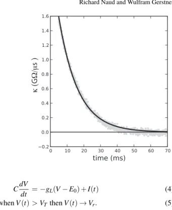
Fig. 3 The filterκ can be measured in real neurons (Jolivet et al, 2006a). Here the shape of the filter is shown as measured in the soma of a pyramidal neuron of the layer 5 of the cortex (gray circles). Data points before 5 ms are not shown because they bear a heavy artefact due to the electrode used for recording. In black is a fit of Eq. 8 with

C= 408 pF andτ= 11.4 ms. κ ( G Ω/μ s ) CdV dt =−gL(V−E0) +I(t) (4) whenV(t)>VTthenV(t)→Vr. (5)

Again, this is the Kirchoff law for conservation of charge. The current injected can either leak out or accumulate on the membrane. Here, the effect of a short cur-rent pulse will cause a transient increase in voltage. This can be seen by looking at the solution of the linear differential equation after a given spike at time ˆt0:

V(t) =E0+ηr(t−tˆ0) + Z t−tˆ₀ 0 κ (s)I(t−s)ds (6) ηr= (Vr−E0)e−t/τΘ(t) (7) κ(t) = 1 Ce −t/τ Θ(t) (8)

whereΘ(t)is the Heaviside function andτ=C/gLis the membrane time constant.

In Eq. 6, three terms combine to make the voltage. The first term is the reversal potential. The second term is the effect of voltage reset which appear through the functionηr. Note that far from the last spike (ˆt0) this term vanishes. The last term

– made of the convolution of the filterκ(t)with the current – is the influence of

input current on the voltage. We see that the voltage is integrating the current but the current at an earlier time has a smaller effect than current at later times. The membrane time constant of real neurons can vary between 10 and 50 ms. The theory of signal processing tells us that the membrane acts as a low-pass filter of the current (Fig. 2). In fact, input current fluctuating slowly is more efficient at driving the voltage than current fluctuating very rapidly.

There is another way to implement the reset. Instead resetting to fixed value, we can see that whenever the voltage equalsVT, there is a sudden decrease in voltage

toVr. According to this point of view the reset is caused by a short negative pulse

of current, which reflects the fact that the membrane loses charge when the neuron sends out a spike. We write the LIF equations differently, using the Dirac delta function (δ(t)):

CdV

dt =−gL(V−E0) +I(t)−C(VT−Vr)

∑

The integrated form is now:

V(t) =E0+

∑

The two different ways to implement the reset yield slightly different formalisms. Even though including the leak made the mathematical neuron model more realistic, it is not sufficient to describe experiments with real neurons. We also need a process to account for adaptation (Rauch et al, 2003; Jolivet et al, 2006b), and this is the topic of the next section.

2 Refractoriness and Adaptation

Refractoriness prevents a second spike immediately after one was emitted. One can distinguish between an absolute and a relative refractory period. The duration of the spike is often taken as the absolute refractory period since it is impossible to emit a spike while one is being triggered. During the absolute refractory period, no spike can be emitted, no matter the strength of the stimulus. During the relative refractory period it is possible to fire a spike, but a stronger stimulus is required. In this case the current required depends on the time since the last spike. Manifestly, the absolute refractory period always precedes the relative refractory period, and the absolute refractory period can be seen as a very strong relative refractory period.

Spike-frequency adaptation, on the other hand, is the phenomenon whereby a constant stimulus gives rise to a firing frequency that slows down in time (Fig. 4). Here it is the cumulative effect of previous spikes that prevents further spiking. In other words: the more a neuron spikes, the less it is likely to spike. How long can this history dependence be? Multiple studies have pointed out that spikes emitted one or even ten seconds earlier can still reduce the instantaneous firing rate (La Camera et al, 2004; Lundstrom et al, 2008).

Refractoriness and adaptation are two similar but distinct effects, and we need to define the difference in precise terms. Although refractoriness mostly affects

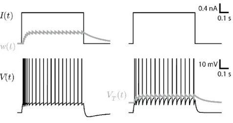
w

Fig. 4 Comparing two simple mechanism of spike-triggered adaptation. A step current (top) is injected in a model with spike-triggered hyperpolarizing current (left) or in a model with moving threshold (right). Both models can produce the same firing patterns, but the voltage trace differs qualitatively.

the earliest times after a spike and adaptation the latest times, this distinction is not adequate: spike-triggered currents can cumulate even at small time scales. It is more convenient to distinguish the two processes based on the history-dependence whereby refractoriness prevents further spiking as a function of time since the last spike only, while adaptation implies a dependency on the time of all the previous spikes. In other words, adaptation is a refractoriness that cumulates over the spikes. Equivalently, refractoriness can be distinguished from adaptation by the type of re-set: a fixed reset like in Eq. 5 leads to dependency on the previous spike only (see Eq. 7) and hence to adaptation. A relative reset allows the effect of multiple spikes to cumulate and can lead to spike-frequency adaptation.

In terms that are compatible with threshold models, both refractoriness and adap-tation can be mediated either by a transient increase of the threshold after each spike or by the transient increase of a hyperpolarizing current. These will be discussed next.

2.1 Spike-Triggered Current

Some ion channels seem to be essential to the action potential but influence very weakly the subthreshold dynamics. Some other ion channels play no role in

defin-ing the shape of the spike, are marginally activated durdefin-ing a spike, and their level of activation decays exponentially after the spike. These are ion channels that can mediate adaptation or refractoriness. Such ion channels have voltage-dependent sen-sitivity to the membrane potential: at high voltage they rapidly open, at low voltage they slowly close. Since a spikes is a short period of high voltage this creates a short jump in the level of adaptation which will slowly decay after the spike. Such a situ-ation can be implemented in the LIF by adding an hyperpolarizing currentwwhich is incremented bybeach time there is a spike and otherwise decays towards zero with a time constantτw:

CdV dt =−gL(V−E0)−w+I(t)−C(VT−Vr)

∑

∑

The above system of equations is a simple mathematical model for a neuron with spike-frequency adaptation. The currentwis triggered by the spikes and will move the membrane potential away from the threshold whenb<0. This equation can be integrated to yield: V(t) =E0+

_∑

whereηa(t) andκ(t) are the same as in Eq. 9. The spike-triggered current that

cumulates over the spikes is reflected in a stereotypical change in voltageηathat

can also cumulate over the spikes. Such a spike-triggered current can also make refractoriness if we replace its cumulative reset by a fixed reset :

τw dw

dt =−w+ (b−w)τw

∑

The shape of the spike after potential can be mediated by a handful of ion chan-nels. Likely candidates for mediating a spike triggered current of the type described above must have a slow to medium activation at supra-threshold potentials and a very slow inactivation or de-activation at subthreshold potentials. An action poten-tial will then induce a small increase in the number of open channels which could cumulate over the spikes. The time constant of the hyperpolarizing currentτwrelates

to the time constant for the closure of the ion channels at subthreshold potentials. Typical examples are: slow potassium currentIK with de-activation time constant

around 30-40 ms (Korngreen and Sakmann, 2000), muscarinic potassium current, IM, with de-activation time constant around 30 to 100 ms (Passmore et al, 2003)

or the calcium-dependent potassium currentIK[Ca]which can have a time constant in the order of multiple seconds (Schwindt et al, 1989). Finally, active dendritic processes can also induce current to flow back into the somatic compartment after each spike (Doiron et al, 2007). In this case the current is depolarizing rather than hyperpolarizing, leading to facilitation rather than adaptation.

2.2 Moving Threshold

Spike-triggered currents are not the only way to implement refractoriness and adap-tation in neuron models. There has been considerable indications that the effective threshold of neurons is dynamic (Fuortes and Mantegazzini, 1962; Azouz and Gray, 2000, 2003; Badel et al, 2008b). If instead of adding a spike-triggered current we let the thresholdVT be dynamic, the threshold can increase byδVT each time there

is a spike and decay exponentially with time constantτT to the minimum threshold V0. This is summarized by the supplementary equations:

τT dVT

dt = −(VT−V0) (18)

whenV(t) ≥ VT(t)thenV(t)→Vr (19)

andVT(t)→VT(t) +δVT. (20)

Again, the moving threshold can implement adaptation (as with Eq.’s 18-20 above) or refractoriness if we replace the relative reset by a fixed reset:VT(t)→ V0+δVT.

It is often possible to find parameters for which a model with a moving threshold will yield the same spikes times than a model with a spike-triggered current. Indeed moving the membrane potential away from the threshold with a spike-triggered cur-rent can be equivalent to moving the threshold away from the membrane potential. In particular, when only the spike times are predicted, we can put Eq.’s 18-20 in the form of Eq. 15 by keeping a fixed threshold and adding toηa(t):

δVTe−t/τTΘ(t). (21)

It is not yet clear which biophysical mechanisms are responsible for moving thresholds. One likely candidate is the sodium channel inactivation (Azouz and Gray, 2000). An increase in sodium channels inactivation can increase the voltage threshold for spike initiation. Inactivated sodium channels de-inactivate with a time constant of 2-6 ms (Huguenard et al, 1988). Furthermore, it is believed that sodium channels can de-inactivate on time scales as long as multiple seconds (Baker and Bostock, 1998).

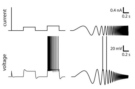
Fig. 5 The responses of the LIF with a single linearized current. A short but strong pulse will generate a jump in potential which will then relaxes with an undershoot. A subthreshold step of current leads to a characteristic overshoot after the onset and an undershoot after the offset of the current. A supra-threshold step of current leads to firing with spike-frequency adaptation. If a sinusoidal wave of increasing frequency is injected in the model, the lowest frequencies and the highest frequencies will be attenuated. In-between frequencies will yield the greatest response.

3 Linearized Subthreshold Currents

There are ion channels influencing principally the shape of the spike, some the re-fractoriness, and others the adaptation of neurons. However, there are also channels whose dynamics depends and influences only the subthreshold potentials. An exam-ple is the hyperpolarization activated cation currentIhwhich start to activate around

-70 mV. Other examples include ion channels making the spike-triggered currents which can also be weakly coupled to the subthreshold voltage. The first-order effect of such currents can be added to the LIF equations (see Ex. 3 or Mauro et al (1970) for details on the Taylor expansion):

CdV dt =−gL(V−E0)−w+I(t) (22) τw dw dt =a(V−Ew)−w (23) ifV(t)>VTthenV(t)→Vr. (24)

Herea regulates the magnitude of the subthreshold current andτw rules the time

constant of the coupling with the voltage.Ewshould correspond to the average

Fig. 6 The shape of the filter κ in the presence of reso-nance. Here the shape of the filter is shown as measured in the apical pyramidal neuron of the layer 5 of the cortex (gray points). Data points before 5 ms are not shown because they bear a heavy artefact from due to the mea-surement electrode. In black is shown a fit of Eq. 22-23 (a

= 13.6 nS,gL= 35.0 nS ,C= 168 pF,τw= 15.5 ms). Data a courtesy of Brice Bathellier.

κ (

G

Ω/μ

s

)

wis said to cause subthreshold facilitation. The response properties will resemble the LIF as (in Fig. 2 and 3) but with a longer impulse-response function. Whena is positive,wis said to generate subthreshold adaptation. For a sufficiently strong positiveawe see the emergence of resonance as shown in Fig. 5.

This system of equations can be mapped to the equations of a damped oscillator with a driving force. It is a well-studied system that comes from the dynamics of a mass hanging on a spring in a viscous medium. We know that this system has three dynamical regimes:

• 4Cτw(gL+a)<(gLτw+C)2overdamped,

• 4Cτw(gL+a) = (gLτw+C)2critically damped,

• 4Cτw(gL+a)>(gLτw+C)2underdamped.

Overdamped and critically damped systems have no resonating frequency. It is only when the system is underdamped that resonance appears. Such resonance is seen in multiple types of neurons, typically in some cortical interneurons (Markram et al, 2004), in mesencephalic V neurons (Wu et al, 2005) and in the apical dendrites of pyramidal neurons (Cook et al, 2007).

What are the main characteristics of a resonating membrane? In the response to the current pulse in Fig. 5 that it is not a single exponential. Instead, the voltage makes a short undershoot before relaxing to the resting potential. Similarly, when the input is a step current, there is a substantial overshoot at the onset and undershoot after the offset of the current. The neuron model resonates around a characteristic frequency for which it will respond with maximal amplitude:

ω= s gL+a Cτw −(gLτw+C)2 4C2_τ2 w . (25)

500 pA

506 pA

2330 pA 2340 pA

10 mV

0.1 s

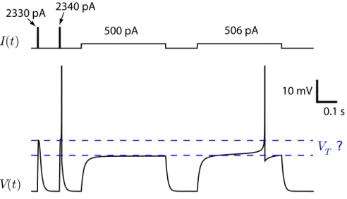
Fig. 7 Where is the voltage threshold? Current pulses and current steps show different voltage thresholds that can not be accounted for by a moving threshold.

Resonating membranes are bandpass filters as we can see from the response to a si-nusoidal wave of increasing frequency (Fig 5). The shape of the filter can be written as: κ(t) =exp(−t/τω) ₁ Ccosωt+ τωτw+1 gL+a sinωt Θ(t) (26)

where the decay time constant is:

τω=

2τwτ

τw+τ. (27)

Figure 6 shows the shape of the filter, as measured in a neuron with resonance.

4 Nonlinear Integrate-and-Fire Models

Do neurons really have a voltage threshold? Imagine that a neuron was to receive a stimulus that brings its membrane potential to a value which triggers the spike but then the stimulus is stopped. The membrane potential would continue to increase even in the absence of stimulus, and produce the action potential. Can we say that a spike is produced whenever the membrane potential reaches this threshold voltage? No. At the earliest times of the action potential, a negative current can veto the spike even though the membrane potential was above the threshold for spike initiation. Another example that makes the conceptualization of a threshold dubious is shown

in Fig. 7. Here the voltage threshold measured from a current pulse is significantly different from the voltage threshold measured with a current step.

Real neurons have sodium ion channels that gradually open as a function of the membrane potential and time. If the channel is open, positive sodium ions flow into the cell, which increases the membrane potential even further. This positive feed-back is responsible for the upswing of the action potential. Although this strong positive feedback is hard to stop, it can be stopped by a sufficiently strong hyperpo-larizing current, thus allowing the membrane potential to increase above the activa-tion threshold of the sodium current.

Sodium ion channels responsible for the upswing of the action potential react very fast. So fast that the time it takes to reach their voltage-dependent level of activation is negligible. Therefore these channels can be seen as currents with a magnitude depending nonlinearly on the membrane potential. This section explores the LIF augmented with a nonlinear term for smooth spike initiation.

4.1 The Exponential Integrate-and-Fire Model

Allowing the transmembrane current to be any function ofV, the membrane dynam-ics will follow an equation of the type:

CdV

dt =F(V) +I(t), (28)

whereF(V)is the current flowing through the membrane. For the perfect IF it is zero (F(V) =0), for the LIF it is linear with a negative slope (F(V) =−gL(V−E0)). We

can speculate on the shape of the non-linearity. The simplest non-linearity would arguably be the quadratic :F(V) =−gL(V−E0)(V−VT)(Latham et al, 2000).

However this implies that the dynamics at hyperpolarized potentials is non-linear, which conflicts with experimental observations. Other possible models could be made with cubic or even quartic functions ofV (Touboul, 2008). An equally simple non-linearity is the exponential function:

F(V) =−gL(V−E0) +gL∆Texp _V−V T ∆T (29)

where∆Tis called the slope factor that regulates the sharpness of the spike initiation.

The Exponential Integrate-and-Fire (EIF; Fourcaud-Trocme et al (2003)) model integrates the current according to Eq. 28 and 29 and resets the dynamics toVr

(i.e.produces a spike) once the simulated potential reaches a value θ. The exact

value ofθ does not matter, as long asθ>>VT+∆T. As in the LIF, we have to

reset the dynamics once we have detected a spike. The value at which we stop the numerical integration should not be confused with the threshold for spike initiation. We reset the dynamics once we are sure the spikehas beeninitiated. This can be

E

_L

V

_T

Fig. 8 Experimental measurement of the nonlinearity for spike initiation. Example of the measured

F(V)in black circles for a layer 5 pyramidal neuron of the barrel cortex. The errorbars indicate one standard error of the mean and the blue line is a fit of Eq. 29. Data is a courtesy of Laurent Badel and Sandrine Lefort (Badel et al, 2008b).

at a membrane potential of 0, 10 mV or infinity. In fact, because of the exponential nonlinearityV goes fromVT+∆T to infinity in a negligible amount of time.

WhichF(V)is the best? This can be measured experimentally (provided that we can estimate membrane capacitance beforehand (Badel et al, 2008a,b)). Fig. 8 shows the functionF(V)as measured in pyramidal neurons of the cortex. Choosing F(V)as a linear plus exponential allow a good fit to the experimental data. Similar curves are observed in neocortex interneurons (Badel et al, 2008a).

5 Unifying Perspectives

We have seen that the LIF can be augmented with mechanisms for refractoriness, adaptation, subthreshold resonances and smooth spike initiation. Models combin-ing these features can be classified in two categories dependcombin-ing on the presence of a non-linearity. This is because the linear system of equations can be integrated ana-lytically, whereas integration is generally not possible for the non-linear systems of equations. When integration can be carried out, the dynamics can be studied with signal processing theory. When this is not possible, the dynamical system is scruti-nized with bifurcation theory.

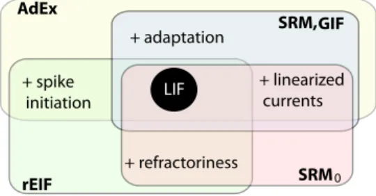
Fig. 9 Generalizations of the LIF include either refractori-ness, adaptation, linearized currents, or smooth spike initiation. Various regroup-ments have various names. For instance, the refractory- Exponential-Integrate-and-Fire (rEIF) regroups refrac-toriness, smooth spike initia-tion and the features of a LIF (Badel et al, 2008b). LIF + adaptation + refractoriness + spike initiation + linearized currents AdEx rEIF SRM GIF 0 SRM,

5.1 The Adaptive Exponential Integrate-and-Fire Model

The simplest way to combine all the features is to add to the EIF model a linearized current with cumulative spike-triggered adaptation:

CdV dt = −gL(V−E0) +gL∆Texp V−VT ∆T +I(t)− N

∑

where each additional currentwican be tuned by adapting its subthreshold coupling

constantaiand its spike-triggered jump sizebi. The simplest version of this

frame-work assumesN=1 and it is known as the Adaptive Exponential Integrate-and-Fire (AdEx; Brette and Gerstner (2005); Gerstner and Brette (2009)). This model com-pares very well with many types of real neurons, as we will see in Sect. 7.

5.2 Integrated Models

For some neurons the spike initiation is sharp enough and can be neglected. In fact, if the slope factor∆→0 in Eq. 30, then the AdEx turns into a linear model with a sharp threshold. As we have seen in Sect. 2, the solution to the linear dynamical system can be cast in the form:

V(t) =E0+ Z ∞ 0 κ (s)I(t−s)ds+

_∑

whereκ(t)is the input filter andηa(t)is the shape of the spike with its

cumula-tive tail. The sum runs on all the spike times{tˆ} defined as the times where the voltage crosses the threshold (V >VT). To be consistent with the processes seen in

10 ms

Fig. 10 Membrane potential recorded from four repetition of the same stimulus. Spikes are missed others are shifted and this variability is intrinsic to the neuron.

the previous sections the functionsκ(t)andηa(t)must be sums of exponentials.

However, for the sake of fitting any type of basis function can be used. For arbitrary shape of the kernelsκ(t)andηa(t), this model is known as the cumulative Spike

Response Model (SRM, Gerstner et al (1996); Gerstner (2008)) or more recently as the Generalized Integrate-and-Fire (GIF, Paninski et al (2004)).

The simplified Spike Response Model (SRM0; Gerstner (2008)) is another

re-lated model worth pointing out. In the SRM0the sum in Eq. 34 extends to the last

spike only. This makes a purely refractory model without spike-frequency adapta-tion. As pointed out in Section 2 purely refractory models are followed by fixed resets.

Figure 9 summarizes the nomenclature for the combinations of generalizations. As we will see in the next section, the formalism of the SRM and SRM0models

bridgesf the gap to a more general class of spiking models where the influence of noise is taken into account.

6 Noise

Variability is ubiquitous in the nervous system. In many ways this variability is seen as a feature rather than a defect (Faisal et al, 2008). It is important therefore not to ignore all the noise, but to listen carefully in order to understand what it is trying to communicate.

In view of the intrinsic probabilistic nature of the neurons, it is difficult to predict the exact spike times because a neuron will fire with some jitter around an average spike time (Fig. 10). Rather, the models of neuronal behaviour must predict the probability to emit a spike in a given time interval. The probabilityp(t)of observing

a spike in a given small interval ofδtdefines the instantaneous firing rate:

p(t) =r(t)δt. (35)

Mathematically speaking,r(t)is a stochastic intensity, a terminology borrowed from the theory of point-processes (Daley and Vere-Jones, 1988). In the context of neuron modelsr(t)is called the firing intensity, instantaneous firing rate. It is also related to the experimentalist concept of a Peri-Stimulus Time Histogram (PSTH).

Chapter 12 describes the implication of noise at the biophysical level. Here we describe how noise influences the level of description of the LIF model. Further-more, we describe a simple framework through which models such as the SRM are related to models of the firing intensityr(t).

6.1 Synaptic Noise

Synaptic noise deals with the inputI(t). In this chapterI(t)refers to the current arriving at the region which is solely responsible for spike initiation. This signal can be seen as being noisy: either because some synaptic events happened without a pre-synaptic spike, or because the unreliability of axonal propagation prevented a pre-synaptic spike from getting to the synapse, or because the variability in vesicle release and receptor channel opening make the amplitude of the postsynaptic event variable. From yet another point of view, one may be interested in the current input coming from an identified subpopulation of pre-synaptic neurons. In this view the rest of the pre-synaptic neurons form a considerable background synaptic noise. In any case, the synaptic noise is added to a deterministic current:

I(t)→I(t) +ξ(t,V) (36) whereξ(t)is the synaptic noise. The dependance of the noise onVis added because synapses make changes in conductance which must be multiplied byV to yield the current. Despite that, the dependance onV can often be neglected and the synaptic noise is considered as a time-dependent currentξ(t).

There are multiple stochastic models of synaptic noise. Maybe the simplest situ-ation takes into account a random ocurence of synaptic events, ˆt(pre)each bringing in an exponentially decaying pulse of current:

ξ(t) =c

_∑

whereτsis the time constant andcis the amplitude of the post-synaptic current

de-cay. If the synaptic events occur randomly with frequencyνe, the mean, the variance

µ≡ hξi=cτsνe (38) σ2≡Var[ξ] = c 2 τsνe 2 (39) h[ξ(t)−µ][ξ(t+s)−µ]i=σ2e−s/τs. (40)

In the limit of small synaptic jumps (c→0) and large frequency of synaptic events (νe→∞), the synaptic noise can be seen as a gaussian noise with exponential

auto-correlation function. The dynamics of such a noise current is often written with the equation: ξ(t+dt) =ξ(t) +(µ−ξ(t)) τs dt+σGt r 2dt τs (41)

whereGt is a random number taken from a standard normal distribution anddt is

the step size. This is called an Ornstein-Uhlenbeck process, a similar equation rules the position of a particle undergoing Brownian motion in an attracting potential. Eq. 41 is the diffusion approximation for synaptic inputs.

6.2 Electrical Noise

Electrical noise groups the thermal noise and the channel noise. The thermal noise (also called Nyquist or Johnson noise) adds fluctuation to the current passing through the membrane due to the thermal agitation of the ions. In this case the variance of the voltage fluctuations at rest is (Manwani and Koch, 1999):kBT B/gL,

wherekBis the Boltzmann constant,T is the temperature andBis the bandwidth

of the system. Thermal noise is not the main source of electrical noise as it is three orders of magnitude smaller than the channel noise (Faisal et al, 2008).

Channel noise is due to the stochastic opening and closing of the ion channels (which itself is of thermal origin). This noise creates fluctuations in current that grow in amplitude with the membrane potential following the activation profile of ion channels. Noise due to the Na-channels responsible for spike initiation can explain how the probability of firing depends on the amplitude of the stimulation when the stimulation consists of a short pulse of current (White et al, 2000). Noise due to Na ion channels is therefore seen as an important source of noise which adds variability to the threshold for spike initiation.

Next section will explore the idea of a stochastic threshold further. Greater details on stochastic models of ion channels will be treated in Chapter 12.

6.3 Generalized Linear Models

Consider the noiseless dynamics forV(t)(as given by the SRM0or SRM) and

VT →θ+ζ(t) (42)

whereθ is the average – or deterministic – threshold, andζ(t)is a zero-mean white noise. This type of noise is called ‘escape noise’ (Gerstner and Kistler, 2002) and relates to the escape rate in the models of chemical reactions (van Kampen, 1992). In this scenario, the probability of finding the membrane potential above the threshold depends solely on the instantaneous difference between the voltage and the average threshold. We can write in general terms that the firing intensity is a nonlinear function of the modelled voltage trace:

r(t) = f(V(t)−θ). (43)

The monotonically increasing nonlinear function f is made of the cumulative dis-tribution function ofζ(t).

Models such as the SRM0or the SRM have an explicit formulation forV(t)that

we can substitute in Eq. 43. These formulations forV(t)require the knowledge of the spiking history. In this case, the firing intensity is dependent on the knowledge of the previous spike times. We will label this intensity differently,λ(t|{tˆ}t), since it

does not equal the PSTH observed experimentally anymore. Writing the convolution operation of Eq. 34 with an asterisk and substituting for the voltage in Eq. 43, we have: λ =f κ∗I+

_∑

When each kernelκ andηaare expressed in a linear combination of basis function

the firing intensity would be a linear model if f was linear. With the nonlinear link-function f, this is instead a Generalized Linear Models (GLM). GLMs all have convenient properties in terms of finding the parameters of the model and estimating the validity of the estimates (McCullagh and Nelder, 1989). One of these properties is that the likelihood of observing a given set of spike times is a convex function of the parameters (when the link function is strictly convex (Paninski, 2004)). This means that it is always possible to find the best set of parameters to explain the data. It is a remarkable fact that only the knowledge of the spike times observed in response to a given stimulus is sufficient to estimate the filter and the shape of the adaptation function.

The GLM model above depends on all the previous spikes, and therefore shows spike-frequency adaptation through the kernelηa(t). By overlooking the possible

in-fluence of cumulative adaptation, it is possible to make a purely refractory stochastic model by dropping the dependence on all the previoius spikes but the last one. This framework allows the theorems of renewal theory (Cox, 1962) to be applied, and to study the behaviour of networks of neurons analytically (Gerstner and Kistler, 2002).

In the same vein, it is possible to ignore completely the refractoriness and con-sider only the filtering of the input:

ν= f(κ∗I). (45) Despite the fact that it appears as too crude an assumption, we can gain considerable knowledge on the functional relationship between external stimuli and neuronal re-sponse (Gazzaniga, 2004). This model referred to as the Linear-Nonlinear Poisson model (LNP) was extensively used to relate the response of single neuron in the retina, thalamus or even cortex as a function of the visual stimulus. When multiple neurons pave the way between the stimulus and the spikes generated by the LNP model, the filter function no longer represents the membrane filter of the cell but rather the linear filter corresponding to successive stages of processing before the signal reaches the neurons.

The mere fact that it is possible to make a decent firing-rate prediction with such a simple model makes strong claim about the role of the neurons and the neural code. A claim that could be challenged by experiments pointing towards missing features. In the next section we further elaborate on the models described in the previous sections. We want to make sure we find thesimplestdescription possible for a given set of experiments, but notsimpler.

7 Advantages of Simple Models

How good are the simple models discussed in this chapter? Before addressing this question one needs to define what is meant by a good model. In an experiment which injects time-varying current in a neuron that otherwise receives no input; what can be reproduced by the model? A model correct in reproducing the averaged firing-rate may not be sufficient to underly the fast computational capabilities of neuron networks (Thorpe et al, 1996). On the other hand, modelling the exact time-course of the membrane potential may not be necessary given that a later neuron only receives the spikes, and no information about the membrane potential of the neuron. Perhaps the best challenge is to predict the occurrence of spikes of a neuron receiving in-vivo-like input. Before evaluating the performance at predicting the spike times, we assess the ability of simple models to reproduce qualitatively the firing patterns observed in various neuron types must be assessed.

7.1 Variety of Firing Patterns

Neurons throughout the nervous system display various types of excitability. The diversity is best illustrated in experiments injecting the same stimulus in cells that otherwise receive no input. By injecting a step current sequentially in multiple cells the observed firing patterns are sure to arise from intrinsic mechanisms. It is com-mon to distinguish qualitatively between the different initial response to the step cur-rent and the diffecur-rent steady state responses (Markram et al, 2004). Consequently,

low

high

low

high

high

low

tonic

adapting

bursting

INITIATION PATTERN

STEAD

Y-ST

ATE P

AT

TERN

Fig. 11 Multiple firing patterns are reproduced by merely tuning the parameters of a simple thresh-old model. Here the AdEx fires with tonic bursts, initial burst, spike-frequency adaptation, or delay. Each set of parameters is simulated on a step current with low (close to current threshold for firing) or high (well above the firing threshold).

the onset of firing is distinguished as being either delayed, bursting or tonic. On the other hand the steady state can be tonic, adapting, bursting or irregular. Sim-ple threshold models can reproduce all the firing patterns observed experimentally (Figure 11). The study of excitability types in such simple models sheds light on the basic principles contributing to the neuronal diversity.

Delayed spiking. Delayed spiking can be due to smooth spike initiation as in the EIF or to linearized subthreshold currents. Indeed, the EIF can produce delayed spiking when the stimulating current is slightly greater thangL(VT−E0−∆).

√

√ √√√ √ √ √_{x x} √_x √ √ √ _√

0.5 s 20 mV

Fig. 12 Overlayed traces of an AdEx model (red) and a fast-spiking interneuron (blue). Most of the spikes are predicted correclty by the model (green check marks) but some extra spike are predicted (red crosses). The subthreshold voltage traces match very well (inset). The data is a courtesy of Skander Mensi and Michael Avermann (?)

to depolarize the membrane further. For instance Eq.’s 22-23 may lead to delayed spiking onset whena<0 andτw>τ.

Bursting. Bursting can arise from many different causes and it is possible to define multiple types of bursting (Izhikevich, 2007). Perhaps the simplest bursting model is the LIF with adaptation (Eq.’s 12-13). The high firing-frequency during a burst increases the adaptation current to a point where the neuron can no longer spike until its level of adaptation has decreased substantially. In this case the inter-burst interval is related to the time constant of adaptation. A hallmark of this type of bursting is the slowing down of the firing during the burst.

Transient spiking. Upon the onset of the stimulus, the neuron fires one or multiple spikes and then remains quiescent, even if the stimulus is maintained for a very long time. Spike-triggered adaptation or a moving threshold cannot account for this pattern. Transient spiking is due to a resonance with a subthreshold current (Fig. 5).

Adaptation. We have seen that spike-frequency adaptation is brought by either hy-perpolarizing currents or a moving threshold which cumulates over multiple spikes. This brief description emphasizes only the most important firing patterns, we will discuss the analysis of the bursting and initial bursting firing patterns further in Section 7.3. For now let us turn to the quantitative evaluation of the predictive power of the mathematical neuron models.

7.2 Spike-Time Prediction

Models of the threshold type can predict the spike times of real neuronsin vitro. It is important to focus on the prediction performance and not simply on reproducing those spike times that were used to calibrate the model parameters. Otherwise, a very complex model could reproduce perfectly the data used for fitting while it would fail completely to reproduce novel stimulus (a phenomenon called overfitting). The correct procedure is therefore to separate the data into a training set and a test set. The first is used for finding the best model parameters and the second to test the performance.

In vitro it is possible to simulate realistic conditions by injecting a fluctuating current in the soma of the neuron. For instance the injected I(t) can be taken to be as in Eq. 37 or Eq. 41 as it would be expected from a high number of synaptic events affecting the soma. This current when injected in the soma drives the neuron to fire spikes. ‘Injecting’ this current in the mathematical neuron models will give a similar voltage trace. After determining the model parameters that yield the best performance on the training set, the neuron model can be used to predict the voltage trace and the spike times on the test set (Figure 12), and can therefore be reproduced with the AdEx model Fig. 11.

Deterministic models such as the SRM0with a dynamic threshold (Jolivet et al,

2006a), the AdEx (Jolivet et al, 2008), the rEIF (Badel et al, 2008b), the GIF (?) or other similar models (Kobayashi et al, 2009) have been fitted to suchin vitro ex-periments and their predictive performance evaluated. To evaluate the performance of deterministic models, the number of predicted spikes that fall within±4 ms of the observed spikes are counted. When discounting for the number of spikes that can be predicted by chance (Kistler et al, 1997), a coincidence factor is obtained ranging from zero (chance level) to one (perfect prediction). This coincidence fac-tor ranged from 0.3 to 0.6 for pyramidal neurons of the layer 5, and from 0.5 to 0.8 for fast-spiking interneurons of the layer 5 of the cortex.

It turns out that these performances are very close to optimal, as we can see if we consider that a real neuron would not reproduce exactly the same spike times after multiple repetitions of the same stimulus (as shown in Fig. 10). The best coincidence factor achievable by the models is the intrinsic reliabilityR, which is the average of the coincidence factor across all pairs of experimental spike trains that received the same stimulus. This value can be seen as an upper bound on the coincidence factor achievable by the mathematical models. Scaling the model-to-neuron coincidence factor by the intrinsic reliability and multiplying by 100 gives a measure of the percentage of the predictable spikes that were predicted. For models like the AdEx or the GIF, this number ranged from 60 to 82 % for pyramidal neurons, and from 60 to 100 % for fast-spiking interneurons. Simpler models do not share this predictive power: the LIF only accounts for 46 to 48 % of the predictable portion of spikes.

Models from the GLM family have been used to predict the spike times of neu-rons in the retina, thalamus or cortex from the knowledge of the light stimulus. Almost perfect prediction can be obtained in the retina and in the thalamus (Keat et al, 2001; Pillow et al, 2005). Furthermore, it has been shown that refractoriness

−50 0 200 400 V (mV) w (pA) 1 4 −50 0 200 400 V (mV) w (pA) 1 5 −70 −70 A B Vr Vr

Fig. 13 Initially bursting (A) and regular bursting (B) trajectories in both phase plane and as a time-series. The initial state of the neuron model before the step current is marked with a cross and is associated with theV-nullcline shown as a dash line. After the step increase in current theV -nullcline shifts upwards (full line). Thew-nullcline is shown in green and the trajectories are shown in blue with each subsequent reset marked with a square. The first and last resets are labeled with their ordinal number. Regular bursting is distinguished from initial bursting by the presence of two voltage resets between the trajectory of the fifth spike and theV-nullcline.

or adaptation is required for good prediction (Berry and Meister, 1998; Pillow et al, 2005; Truccolo et al, 2010). Furthermore, the quality of the prediction can be im-proved by taking into account the coupling between adjacent cells (Pillow et al, 2008).

7.3 Ease of Mathematical Analysis

The greater simplicity of the mathematical neuron models discussed in this chapter have another advantage: the ease of mathematical analysis. This is particularly ad-vantageous for studying neuron networks and for investigating synaptic plasticity. This is a vast field of study where many macroscopic properties of neuron networks can be scrutinized: learning, oscillations, synchrony, travelling waves, coding, and possibly other (see Hoppensteadt and Izhikevich (1997); Dayan and Abbott (2001), and Gerstner and Kistler (2002) for a good introduction to the topic). Paving the way to these exciting fields, mathematical analysis has yield important insights that relate the function of single neurons with that of networks.

The characteristic of the response to various types of stimulations can often be described in mathematical terms. For a constant current I, the firing frequency of the LIF is given by (see Ex. 5):

ν= τln gL(Vr−E0)−I gL(VT−E0)−I −1 . (46)

The mean frequency when the current is an Ornstein-Uhlenbeck process (Eq. 41) can be written as an integral formula (Johannesma, 1968):

ν= " τ √ π Z √ τ(gL(VT−E0)−µ)/(σ √ 2τs) √ τ(gL(Vr−E0)−µ)/(σ √ 2τs) ex2[1+erf(x)]dx #−1 (47)

where erf(x)is the error function. When the non-linearity for spike initiation is taken into account, it is not possible to arrive at exact solutions anymore. Yet, for some parameter values there are approximations that can be worked in. This way, approx-imated solutions can be written for the EIF or the AdEx receiving gaussian white noise (Fourcaud-Trocme et al, 2003; Richardson, 2009). When there is a strong ef-fect of adaptation it is not possible to arrive at closed-form solutions forνand one

must rely on numerical integration of the appropriate Fokker-Planck equations can be used (Muller et al, 2007; Toyoizumi et al, 2009).

Along these lines, the observed types of firing patterns can be related with the parameter values through bifurcation theory (see Chapter 13). We will illustrate this with an example in the AdEx model: distinguishing initial bursting from a regular bursting using phase plane analysis.

Repetitive bursting is created by constantly alternating between slow and fast in-terspike intervals. When the injection is a step increase in current (as with Fig. 11) this corresponds to a sudden shift of theV-nullcline (i. e.the set of points where

dV

dt =0) in the phase plane. Before the step, the state of the neuron is at the stable

fixed point which is sitting at the intersection between teV- and thew-nullcline. Af-ter the step, the stable fixed point has disappeared and this results in repetitive firing. The distinction between an initially bursting AdEx model and a regular bursting one is made by considering the location of the resets in the phase plane. Fig 13 shows that both types of bursting have spike resets above and below theV-nullcline. Re-setting above theV-nullcline brings a much larger interspike interval than resetting below. To achieve this, a spike reset above theV-nullcline must be able to make at least one spike reset below theV-nullcline before being mapped above again. This is seen in Fig. 13B where there is sufficient space below theV-nullcline and above the trajectory of the fifth spike for at least one reset. This leads the repetitive bursting of two spikes. On the other hand, in Fig. 13A the fourth spike – which was reset above theV-nullcline – is followed bys another reset above theV-nullcline. This leads to the end of the initial burst which is followed only by long interspike intervals. By staring at the phase planes in Fig. 13, one can conclude that a higher voltage reset helps to bring about repetitive bursting.

Similar conclusions can be drawn for all the firing patterns (Naud et al, 2008). Furthermore, it is sometimes possible to have analytical expressions relating the parameter values and the firing patterns (Touboul, 2008). Such conclusions are pos-sible mainly because the complexity of the model was kept low. Indeed, the struc-ture of firing patterns have been studied in other simple models (Izhikevich, 2007; Mihalas¸ and Niebur, 2009).

8 Limits

The neuron models presented in this chapter present an idealized picture. The first idealization is that all these models consider the neuron as a point with no spatial structure. This point could represent the axon initial segment where the spike is initiated. However, real neurons receive input distributed not only in the soma but also in their dendritic arborizations. Now, dendrites bring multiple types of non-linear interactions between the inputs. Dendritic ion channels combine with basic properties of AMPA, GABA and NMDA synapses to make dendritic output to the soma dependent on the spatio-temporal pattern of excitation. Spatially extensive models (see Chapter 11) may be required to correctly translate input spikes into current arriving to the axon initial segment, but to what extent? This remains to be addressed experimentally.

Another central assumption prevalent throughout this chapter is that the spike does not change its length or shape with different stimuli. While this is seen as a good approximation for cortical neurons firing at low frequency (Bean, 2007), some neurons have action potential shapes that vary strongly as a function of either stimu-lus, firing frequency or neuromodulation. For instance, the interneurons taking part in the motor pattern generation of flight in locusts display spikes that reduce by half their amplitude and width when part of a burst of activity (Wolf and Pearson, 1989). Similarly, half-blown spikes are observed frequently in the lobster stomatogastric pattern generator (Clemens et al, 1998) or in complex spikes of cartwheel cells in the dorsal cochlear nucleus (Golding and Oertel, 1997).

The simple models described in this chapter can be seen as a high-level descrip-tion of the complex biophysical mechanisms mediated by ion channels, ion pumps, and various chemical reactions involving neurotransmitters. At this level of descrip-tion the molecular cascades for the effect of – for example – acetylcholine are not modelled. Though the effect of neuromodulators can be calibrated and cast in stereo-typical modification of the simple model (Slee et al, 2005), it is not an intrinsic feature and the calibration has to be performed for each scenario. Complex bio-chemical as well as biophysical models are the norm if pharmacological procedures are studied (see Chapter 17-18).

To conclude, simple neuron models captured essential features that are required for transducing input into spikes. If we bear in mind the inherent limitations, the study of simple neuron models will keep on bringing new insights about the role of single neurons. In particular, the roles of adaptation and variability are only starting to be sized.

9 Further Reading

Spiking Neuron Modelsuses single-neuron models as a building block for studying fundamental questions such as neuronal coding, signal transmission, dynamics of neuronal populations and synaptic plasticity. (Gerstner and Kistler, 2002).

Dynamical Systems in Neuroscience. Neuron models are made of systems of differential equations, this book makes a very didactic approach to the mathematical theory associated with such dynamical systems (Izhikevich, 2007).

Exercices

1. WithEw=E0, cast Eq.’s 22-23 in the form of Eq. 34.

Solution: ηa=0 κ(t) =k+eλ+t+k−eλ−t where λ±= 1 2τ τw −(τ+τw)± p (τ+τw)−4τ τw(gL+a)/gL and k±=± λ±τw+1 Cτw(λ+−λ−) .

2. If we connect a dendritic compartment to a LIF point neuron, the dynamics of the system obey:

CdV

dt =−GL(V−VL) +Gc(Vd−V) +I Cd

dVd

dt =−Gd(V−Ed) +Gc(V−Vd)

wheregcis the conductance coupling the LIF compartment with membrane

po-tentialV to the dendritic compartment with potentialVd. The leak conductance,

the capacitance and the reversal potential for the dendritic compartment aregd, CdandEd, respectively. How should you definew,a,gL,E0,Ewandτwto show

that this situation is equivalent to Eq.’s 22-23?

Solution: w=GcVd,gL=GL+Gc,E0=GLVL/(GL+Gc),a=Gd+Gc,Ew= EdGd/(Gc+Gd),τw=Cd/Gd.

3. Reduce the Hodgkin-Huxley equations (see Chapter 11) to the AdEx model. Start with the single-compartment Hodgkin and Huxley equations:

CdV dt =−gm(V−Em)−gNam 3_h(V−E Na)−gKn4(V−EK), (48) τx(V) dx dt =−x+x∞(V), (49)

withxbeing any of the gating variablesm,horn. Solution:

i) Assume thatτm(V)<<C/gL.

ii) Assume that when the voltage reaches some relatively high value (e.g. -10 mV) there is a spike being emitted and the voltage is reseted toVr, while the

potassium activation make a stereotypical change:n→n+δn.

iii) Assume that the sodium inactivation variable plays no role sub-threshold and during the spike initiation:h(t) =h0.

iv) There remains only subthreshold dynamics and spike initiation, therefore the dynamics ofh,nandIK can be linearized aroundE0(multivariate taylor

expan-sion). The resulting system is:

CdV dt = I−gL(V−E0)−gNah0m 3 ∞(V)(V−ENa)−w (50) τw dw dt = aw(V−E0)−w (51) ifV >0mV then V =Vr,w=w+b. (52) withw(t) =4gK(n(t)−n∞(E0))n3∞(E0)(E0+EK),a=4gKn∞(E0)3(E0+EK)∂_∂n_V∞ E0 , τw=τn(E0),b=4gKδnn3∞(E0)(E0−EK).

4. Computer aided exercice. Build a simple GIF model to reproduce all the firing patterns in Fig. 11.Hint:let kernelsη(t)andκ(t)each be constituted of two exponentials.

5. Derive equation 46 starting from Equations 6-8 with a constant current. Hint: Callν−1the time it takes to go from the reset to the threshold. WithIconstant the integrals can be computed explicitly.

References

Azouz R, Gray C (2000) Dynamic spike threshold reveals a mechanism for coinci-dence detection in cortical neurons in vivo. Proc National Academy of Sciences USA 97:8110–8115

Azouz R, Gray CM (2003) Adaptive coincidence detection and dynamic gain con-trol in visual cortical neurons in vivo. Neuron 37:513–523

Badel L, Lefort S, Berger T, Petersen C, Gerstner W, Richardson MJE (2008a) Ex-tracting non-linear integrate-and-fire models from experimental data using dy-namic i-v curves. Biological Cybernetics 99:361–370

Badel L, Lefort S, Brette R, Petersen C, Gerstner W, Richardson M (2008b) Dy-namic i-v curves are reliable predictors of naturalistic pyramidal-neuron voltage traces. J Neurophysiol 99:656–666

Baker MD, Bostock H (1998) Inactivation of macroscopic late na+ current and characteristics of unitary late na+ currents in sensory neurons. J Neurophysiol

80(5):2538–49

Bean BP (2007) The action potential in mammalian central neurons. Nat Rev Neu-rosci 8(6):451–65

Berry M, Meister M (1998) Refractoriness and neural precision. J of Neuroscience 18:2200–2211

Brette R, Gerstner W (2005) Adaptive Exponential Integrate-and-Fire Model as an Effective Description of Neuronal Activity. Journal of Neurophysiology 94(5):3637–3642

Clemens S, Combes D, Meyrand P, Simmers J (1998) Long-term expression of two interacting motor pattern-generating networks in the stomatogastric system of freely behaving lobster. Journal of neurophysiology 79(3):1396–408

Cook EP, Guest JA, Liang Y, Masse NY, Colbert CM (2007) Dendrite-to-soma in-put/output function of continuous time-varying signals in hippocampal ca1 pyra-midal neurons. J Neurophysiol 98(5):2943–2955, DOI 10.1152/jn.00414.2007 Cox DR (1962) Renewal theory. Methuen, London

Daley D, Vere-Jones D (1988) An introduction to the theory of point processes. Springer, New York

Dayan P, Abbott LF (2001) Theoretical Neuroscience. MIT Press, Cambridge Doiron B, Oswald A, Maler L (2007) Interval coding. ii. dendrite-dependent

mech-anisms. Journal of Neurophysiology 97:2744–2757

Faisal A, Selen L, Wolpert D (2008) Noise in the nervous system. Nature reviews Neuroscience 9(4):292

Fourcaud-Trocme N, Hansel D, Vreeswijk CV, Brunel N (2003) How spike gener-ation mechanisms determine the neuronal response to fluctuating inputs. Journal of Neuroscience 23(37):11,628–11,640

Fuortes M, Mantegazzini F (1962) Interpretation of the repetitive firing of nerve cells. J General Physiology 45:1163–1179

Gazzaniga MS (2004) The cognitive neurosciences, 3rd edn. MIT Press, Cambridge, Mass.

Gerstner W (2008) Spike-response model. Scholarpedia 3(12):1343

Gerstner W, Brette R (2009) Adaptive exponential integrate-and-fire model. Schol-arpedia 4(6):8427

Gerstner W, Kistler W (2002) Spiking neuron models. Cambridge University Press New York

Gerstner W, van Hemmen J, Cowan J (1996) What matters in neuronal locking? Neural computation 8:1653–1676

Golding NL, Oertel D (1997) Physiological identification of the targets of cartwheel cells in the dorsal cochlear nucleus. Journal of neurophysiology 78(1):248–60 Hoppensteadt FC, Izhikevich EM (1997) Weakly connected neural networks.

Springer

Huguenard JR, Hamill OP, Prince DA (1988) Developmental changes in na+ con-ductances in rat neocortical neurons: appearance of a slowly inactivating compo-nent. J Neurophysiol 59(3):778–95

Izhikevich EM (2007) Dynamical systems in neuroscience : the geometry of ex-citability and bursting. MIT Press, Cambridge, Mass.

Johannesma P (1968) Diffusion models of the stochastic acticity of neurons. In: Neural Networks, Springer, Berlin, pp 116–144

Jolivet R, Rauch A, L¨uscher HR, Gerstner W (2006a) Integrate-and-fire models with adaptation are good enough. In: Weiss Y, Sch¨olkopf B, Platt J (eds) Advances in Neural Information Processing Systems 18, MIT Press Cambridge, pp 595–602 Jolivet R, Rauch A, Luscher HR, Gerstner W (2006b) Predicting spike timing of

neocortical pyramidal neurons by simple threshold models. J Comput Neurosci 21(1):35–49

Jolivet R, Kobayashi R, Rauch A, Naud R, Shinomoto S, Gerstner W (2008) A benchmark test for a quantitative assessment of simple neuron models. J Neuro-science Methods 169:417–424

van Kampen NG (1992) Stochastic processes in physics and chemistry, 2nd edn. North-Holland, Amsterdam

Keat J, Reinagel P, Reid RC, Meister M (2001) Predicting every spike: a model for the responses of visual neurons. Neuron 30(3):803–817

Kistler WM, Gerstner W, van Hemmen JL (1997) Reduction of Hodgkin-Huxley equations to a single-variable threshold model. Neural Comput 9:1015–1045 Kobayashi R, Tsubo Y, Shinomoto S (2009) Made-to-order spiking neuron model

equipped with a multi-timescale adaptive threshold. Frontiers in Computational Neuroscience 3:9

Korngreen A, Sakmann B (2000) Voltage-gated k+ channels in layer 5 neocorti-cal pyramidal neurones from young rats:subtypes and gradients. The Journal of Physiology 525(3):621–639

La Camera G, Rauch A, L¨uscher HR, Senn W, Fusi S (2004) Minimal models of adpated neuronal responses to in-vivo like input currents. Neural Computation 16:2101–2104

Lapicque L (1907) Recherches quantitatives sur l’excitation electrique des nerfs trait´ee comme une polarization. J Physiol Pathol Gen 9:620–635, Cited in H.C. Tuckwell,Introduction to Theoretic Neurobiology. (Cambridge Univ. Press, Cam-bridge, 1988)

Latham PE, Richmond B, Nelson P, Nirenberg S (2000) Intrinsic dynamics in neu-ronal networks. I. Theory. J Neurophysiology 83:808–827

Lundstrom B, Higgs M, Spain W, Fairhall A (2008) Fractional differentiation by neocortical pyramidal neurons. Nature Neuroscience 11(11):1335–1342

Manwani A, Koch C (1999) Detecting and estimating signals in noisy cable struc-tures, I: Neuronal noise sources. Neural Computation 11:1797–1829

Markram H, Toledo-Rodriguez M, Wang Y, Gubta A, Silbrberg G, Wu C (2004) Interneurons of the neocortical inhibitory system. Nature Reviews Neuroscience 5:793–807

Mauro A, Conti F, Dodge F, Schor R (1970) Subthreshold behavior and phenomeno-logical impedance of the squid giant axon. J Gen Physiol 55(4):497–523 McCullagh P, Nelder JA (1989) Generalized linear models, vol 37, 2nd edn.

Chap-man and Hall, London

Mihalas¸ S, Niebur E (2009) A generalized linear integrate-and-fire neural model produces diverse spiking behaviors. Neural computation 21(3):704–18

Muller E, Buesing L, Schemmel J, Meier K (2007) Spike-frequency adapting neu-ral ensembles: beyond mean adaptation and renewal theories. Neuneu-ral Comput 19(11):2958–3010, DOI 10.1162/neco.2007.19.11.2958

Naud R, Marcille N, Clopath C, Gerstner W (2008) Firing patterns in the adaptive exponential integrate-and-fire model. Biological Cybernetics

Paninski L (2004) Maximum likelihood estimation of cascade point-process neural encoding models. Network: Computation in Neural Systems

Paninski L, Pillow J, Simoncelli E (2004) Maximum likelihood estimate of a stochastic integrate-and-fire neural encoding model. Neural computation 16:2533–2561

Passmore G, Selyanko A, Mistry M, Al-Qatari M, Marsh SJ, Matthews EA, Dick-enson AH, Brown TA, Burbidge SA, Main M, Brown DA (2003) Kcnq/m cur-rents in sensory neurons: significance for pain therapy. Journal of Neuroscience 23(18):7227–7236

Pillow J, Paninski L, Uzzell V, Simoncelli E, EJChichilnisky (2005) Prediction and decoding of retinal ganglion cell responses with a probabilistic spiking model. J Neuroscience 25:11,003–11,023

Pillow JW, Shlens J, Paninski L, Sher A, Litke AM, Chichilnisky EJ, Simoncelli EP (2008) Spatio-temporal correlations and visual signalling in a complete neuronal population. Nature 454(7207):995–1000

Rauch A, Camera GL, Luscher H, Senn W, Fusi S (2003) Neocortical pyramidal cells respond as integrate-and-fire neurons to in vivo-like currents. Journal of neu-rophysiology 90:1598–1612

Richardson MJE (2009) Dynamics of populations and networks of neurons with voltage-activated and calcium-activated currents. Phys Rev E Stat Nonlin Soft Matter Phys 80(2 Pt 1):021,928

Schwindt, Spain W, Crill W (1989) Long-lasting reduction of excitability by a sodium-dependent potassium current in cat cortical neurons. Journal of Neuro-science 61(2):233–244

Slee SJ, Higgs MH, Fairhall AL, Spain WJ (2005) Two-dimensional time coding in the auditory brainstem. J Neurosci 25(43):9978–88

Stein RB (1965) A theoretical analysis of neuronal variability. Biophys J 5:173–194 Thorpe S, Fize D, Marlot C (1996) Speed of processing in the human visual system.

Nature 381:520–522

Touboul J (2008) Bifurcation analysis of a general class of nonlinear integrate-and-fire neurons. SIAM Journal on Applied Mathematics 68(4):1045–1079

Toyoizumi T, Rad K, Paninski L (2009) Mean-field approximations for coupled populations of generalized linear model spiking . . . . Neural computation Truccolo W, Hochberg LR, Donoghue JP (2010) Collective dynamics in human

and monkey sensorimotor cortex: predicting single neuron spikes. Nature Neuro-science 13(1):105–111

White JA, Rubinstein JT, Kay AR (2000) Channel noise in neurons. Trends in Neu-roscience 23(3):1–7

Wolf H, Pearson K (1989) Comparison of motor patterns in the intact and deaf-ferented flight system of the locust. iii: Patterns of interneuronal activity.

Jour-nal of comparative physiology A, Sensory, neural, and behavioral physiology 165(1):61–74

Wu N, Enomoto A, Tanaka S, Hsiao CF, Nykamp DQ, Izhikevich E, Chandler SH (2005) Persistent sodium currents in mesencephalic v neurons participate in burst generation and control of membrane excitability. J Neurophysiol 93(5):2710–22, DOI 10.1152/jn.00636.2004