City, University of London Institutional Repository
Citation
:
Zu, Y. (2015). Nonparametric specification tests for stochastic volatility models based on volatility density. Journal of Econometrics, 187(1), pp. 323-344. doi:10.1016/j.jeconom.2015.02.045
This is the accepted version of the paper.
This version of the publication may differ from the final published
version.
Permanent repository link:
http://openaccess.city.ac.uk/8090/Link to published version
:
http://dx.doi.org/10.1016/j.jeconom.2015.02.045Copyright and reuse:
City Research Online aims to make research
outputs of City, University of London available to a wider audience.
Copyright and Moral Rights remain with the author(s) and/or copyright
holders. URLs from City Research Online may be freely distributed and
linked to.
City Research Online: http://openaccess.city.ac.uk/ [email protected]
Nonparametric specification tests for stochastic
volatility models based on volatility density
∗
Yang Zu
†City University London
March 10, 2015
Abstract
This paper develops a specification test for stochastic volatility models by
com-paring the nonparametric kernel deconvolution density estimator of an integrated
volatility density with its parametric counterpart. L2 distance is used to measure
the discrepancy. The asymptotic null distributions of the test statistics are
estab-lished and the asymptotic power functions are computed. Through Monte Carlo
simulations, the size and power properties of the test statistics are studied. The
tests are applied to an empirical example.
JEL Classification: C58, C12, C14.
Keywords: nonparametric tests, kernel deconvolution estimator, stochastic volatility
model.
1
Introduction
Consider the following continuous-time stochastic volatility model:
dXt=σtdBt,
dσt2 =b(σt2)dt+a(σt2)dWt,
(1)
∗I wish to thank the co-editor Yacine A¨ıt-Sahalia, the associate editor and three anonymous referees for
careful reading the manuscript and providing helpful comments and suggestions, which greatly improve the paper. This paper is revised from a chapter of my PhD thesis at the University of Amsterdam, I wish to thank my supervisor Peter Boswijk for helpful advice and encouragement. I also wish to thank Aurore Delaigle for the helpful email correspondence, Bert van Es and Dennis Kristensen for fruitful discussions and suggestions. Helpful comments from Peter Spreij, Cees Diks, Jan de Gooijer, Philippos Papadopoulos, and the session participants of the 10th World Congress of the Econometric Society are also gratefully acknowledged. All remaining errors are my own.
†Email: [email protected]. Department of Economics, City University London, Northampton
whereB andW are two independent standard Brownian motion processes. X is assumed
to be observed discretely at ti =i∆, for i = 0,1, . . . , n, ∆ is assumed to be fixed, while
σ2 is assumed to be unobservable.
The model (1) is used to describe the evolution of asset prices in financial markets.
Nonparametric estimation of continuous-time stochastic volatility models has been
con-sidered in Franke et al. (2003), Reno (2006), Reno (2008), Kanaya and Kristensen (2015)
and Comte et al. (2010), among others.
Assume that in the stochastic volatility model (1), the true model is characterized by
the functions {b0(.), a0(.)}, and let a parametrization of the model be:
{b(.;θ), a(,;θ), θ∈Θ⊆Rk}.
This paper aims to study the problem of testing the null hypothesis
H0 :{∃θ0 ∈Θ, b(.;θ0) =b0(.), a(.;θ0) = a0(.)},
vs. (2)
H1 :{b(.;θ)6=b0(.), a(.;θ0)6=a0(.),∀θ∈Θ}.
If σ2 was observable (in discrete time), this problem would be reduced to a specifica-tion test problem for diffusion processes. For example, A¨ıt-Sahalia (1996) proposed a
specification test for diffusion processes by comparing the nonparametric kernel density
estimate of the stationary density of the process with its parametric counterpart. His
test statistic for the present model would be as follows:
Tn = n X
i=1
ˆ
π σi2−πσi2; ˆθn
2
, (3)
where ˆπ(x) = Pni=1K((x−σi2)/h)/(nh) is the nonparametric kernel density estimator of the stationary volatility density,π(x;θ) is the corresponding parametric density under the null hypothesis, and ˆθn is an estimator of the parameters. The sum in (3) is over
the grid of observations. However, the unobservability of σ2 in the stochastic volatility model (1) makes this test not applicable to the problem in this paper.
Although the volatility process is not observable in model (1), Van Es et al. (2003)
notice that the volatility density of the model can still be estimated nonparametrically
by a deconvolution kernel density estimator using the observed log return data because
the discretized stochastic volatility model can be rewritten into a convolution model: let
sequence:
yi :=
1
∆1/2 Xti−Xti−1
= 1
∆1/2
Z ti
ti−1
σsdBs
∼ N
0, 1 ∆
Z ti
ti−1
σ2sds
for i = 1, . . . , n, where ∼ means “distributed as”. Define ηi := Rti
ti−1σ
2
sds/∆ and use εi,
i= 1, . . . , nto denote independent and identically distributed standard normal variables.
The above equation can be written as:
yi =η
1/2
i εi, i= 1, . . . , n.
Squaring both sides and taking the logarithms,
logyi2 = logηi+ logε2i, i= 1, . . . , n, (4)
such that the variable logy2
i is the convolution of logηi with logε2i, which has a completely
known log chi-square distribution.
In statistics, model (4) is known as a measurement error model — the signal logηi
is measured with a noise logε2
i, and only logyi2 is observed. Recovering the density
of the signal logηi from the observed logyi2’s is called density deconvolution. Density
deconvolution can be done in several ways, see Meister (2009) for a review. Denoting the
density function of logηiasg(x), it can be estimated by the following kernel deconvolution
estimator:
ˆ
g(x) = 1 2π
1 n
n X
j=1
Z +∞
−∞
φK(th)
φk(t)
e−it(x−logy2j)dt,
where the definitions of φK and φk are left in Section 2.
Motivated by these studies, this paper proposes to test the hypothesis H0 against
H1 by comparing the parametric estimate and the nonparametric kernel deconvolution estimate of the stationary density function of logηi. Notice that the asymptotic scheme
considered in this paper is different from that of Van Es et al. (2003), where both the
in-fill and long span asymptotic schemes are used. In this paper the sampling interval
∆ is assumed to be fixed and only a long span asymptotic scheme is used. This is
consistent with the usual practice in financial econometrics that a stochastic volatility
model is usually used to model returns sampled at daily or lower frequency. Under our assumption, the object of comparison is not exactly the stationary volatility density but
the density function of logηi := log
Rti
ti−1σ
2
sds/∆
– the log integrated volatility density.
as the corresponding parametric density function under the null hypothesis. The test
statistic could be formulated by calculating theL2 distance between ˆg(x) and g(x; ˆθ),
T0 =
Z
R
ˆ
g(x)−g(x; ˆθ) 2
dx.
The actual testing problem studied in this paper can be expressed as follows:
H00 :{∃θ0 ∈Θ, g(.;θ0) = g0(.)} vs. H01 :{g(.;θ)6=g0(.),∀θ ∈Θ}. (5)
The reformulated testing problem (5) is not equivalent to the original problem in (2),
which tests H0 against H1. There are certain deviations in H1 can not be detected by the reformulated testing problem. For example, this test will not be able to detect
a volatility model with misspecified transitional density, but with a correctly specified
marginal density. To address this problem, a possible extension to base the test on the
bivariate volatility density is discussed in Section 5.4.
The idea of comparing parametric and nonparametric estimates for specification tests
is not new. Bickel and Rosenblatt (1973) and H¨ardle and Mammen (1993), among others,
made early contributions. Nonparametric tests with weakly dependent data were studied
by Fan (1994), Fan and Ullah (1999), Fan and Li (1999), and A¨ıt-Sahalia et al. (2001),
among others. Nonparametric specification tests for diffusion processes were investigated
by A¨ıt-Sahalia (1996), Hong and Li (2005), Corradi and Swanson (2005), Chen et al. (2008), A¨ıt-Sahalia et al. (2010) and A¨ıt-Sahalia and Park (2012), among others.
Spec-ification tests involving a deconvolution kernel estimator is relatively new, see Butucea
(2007) and Holzmann et al. (2007).
There are several existing tests for stochastic volatility models. Early contributions
include the moment restrictions based tests (such as (Gallant et al., 1997)). Recent
contributions include Corradi and Distaso (2006), who propose testing the specification
of stochastic volatility models based on the moment information of realized volatility
measures, and Corradi and Swanson (2011), who propose basing the test on the one-step
predictive density of observed series. Zu and Boswijk (2009) propose tests based on the density function and distribution function of the observed returns.
It may seem natural to perform the test based on the observable return distributions
and/or densities. However, the volatility density based test considered in this paper is
useful in detecting certain types of local deviations to the null model. This is because the
return density is a convolution of the volatility density with the log chi-square density.
It can happen that two volatility densities at a certain L2 distance will become very close to each other after the convolution, and become very hard to distinguish by looking
at the densities of the return densities. Example 2 of Holzmann et al. (2007) gives a
specified to converge to the null model at a certain rate, but after taking a convolution
operation with a Laplace density, the convergence rate could become arbitrarily faster. In
this case, the testing problem becomes harder after the convolution and it would be more
efficient to formulate the test in terms of the volatility density. In practice, since it is not
known which kind of deviation the data generating process might have, the test proposed
in this paper could be served as a useful complement to the return density/distribution
based tests.
The methodology proposed in this paper only test statistical goodness-of-fit of a
stochastic volatility model, it does not consider the model tractability and the related
issues, which are important in determining a model specification in practical financial applications, say option pricing. Thus it is important that the test developed in this
paper be interpreted appropriately and used with caution when invalidating a stochastic
volatility model.
Model (1) does not allow for a drift term and a jump term, which is not consistent
with empirical facts observed in realistic financial returns. Nevertheless, the model is still
useful as it can be applied to the series which has been demeaned and has the jumps been
filtered out. This issue will be discussed further in detail in Section 5.2. By considering
model (1) the attention is focused on the (mis)specification of the volatility process.
This paper is organized as follows. Deconvolution kernel density estimation for the log integrated volatility density is discussed in Section 2. The parametric estimate of the
log integrated volatility density is discussed in Section 3. The log integrated volatility
density usually does not have an explicit formula. This section also discusses methods
of approximating the log integrated volatility density. The test statistic, its asymptotic
null distribution, and the asymptotic power of the test under fixed and local
alterna-tives are studied in Section 4. A parametric bootstrap procedure is also proposed in this
section to approximate the finite sample null distribution. Section 5 discusses possible
extensions along different directions. Section 6 performs Monte Carlo simulations. The
size and power properties of the tests are studied under various realistic scenarios. The test is applied to a real example in Section 7. Section 8 concludes the paper. Technical
assumptions are stated in Appendix A. The proofs are collected in Appendix B.
Tech-nical lemmas used in the proofs are collected in Appendix C. An alternative method of
approximating the parametric volatility density is discussed in Appendix D.
In this paper, φg(t) =
R∞
−∞e
itxg(x)dx is defined as the Fourier transform of function
g(x); the inverse Fourier transform is defined as g(x) = (2π)−1R−∞+∞e−itxφ
g(x) dt. An
integral R with no upper and lower limit implicitly means it is an integral over the real
line. −→d is used to denote convergence in distribution and ∼ to denote “distributed as”.
kfkp := (R |f(x)|pdx)1/p, p >0 denotes thepth norm of functionf, provided that it exists.
By definition kfkp is always nonnegative, and kfkp = 0 only when f(x) = 0 almost
in this paper have strictly positive norms. g ∗ k(x) = R
g(x− y)k(y)dy denotes the
convolution of g(.) and k(.). The volatility process in this paper is always used to refer
to the σ2 process, not the σ process.
2
Nonparametric log integrated volatility density
Assume that the density functions of logy2i, logηi and logε2i exist, denoted asf(.),g(.),
and k(.), respectively. Equation (4) implies the following convolution relationship:
f(x) =g∗k(x).
When Yi := logy2i, i = 1, . . . , n are observable and k(x) is fully known, the density
function g(x) can be estimated by the deconvolution kernel density estimator:
ˆ
g(x) = 1 2π
1 n
n X
j=1
Z +∞
−∞
φK(th)
φk(t)
e−it(x−Yj)dt,
where φK is the Fourier transform of a kernel function K and φk(t) is the characteristic
function corresponding to k(x). The kernel deconvolution estimator was first proposed
for the measurement error model by Carroll and Hall (1988) and Stefanski and Carroll
(1990).
If
νh(x) :=
1 2π
Z +∞
−∞
φK(t)
φk(t/h)
e−itxdt,
is defined to be the deconvolution kernel function, the estimator can be written in a kernel
form:
ˆ
g(x) = 1 nh
n X
j=1
νh
x−Yj
h
. (6)
It is known that νh(x) is a real-valued function when φK(t) is even and real (see, e.g.,
Stefanski and Carroll (1990)).
The error term logε2
i follows a log chi-square distribution. Its probabilistic properties
can be found in e.g. Van Es et al. (2005) and Comte (2004). In particular, the
charac-teristic function of the log chi-square distribution is φk(t) = 2itΓ (1/2 + it)/ √
π; the tail
decay rate of its modulus function is described by|φk(t)|= √
2 exp(−π|t|/2)(1 +O(1/|t|))
as |t| → ∞. According to Fan (1991), this error belongs to the so-called super-smooth
errors because the tail of the modulus function decays exponentially fast.
The kernel function considered first in this paper is the so-called sinc kernel:
K(x) =
(
sin (x)/(πx) ifx6= 0,
The sinc kernel is also called Fourier Integral kernel. The usage of this kernel in
den-sity deconvolution dates back to Stefanski and Carroll (1990). Its Fourier transform is
φK(t) =I{|t|61}, where I{·}is an indicator function. The simplicity of φK(t) aids the
computation and thus the sinc kernel is favoured in theoretical literature (e.g. Butucea
(2007), among others). It is a so-called “infinite order” kernel, see Delaigle and Hall
(2010) Section 3.1 for a detailed discussion about this property in general and in the
context of kernel deconvolution.
Although R K(x) = 1, it is not a proper probability density because it takes negative
values. A main drawback of the sinc kernel is its numerical stability; it often causes
unwanted oscillations in the estimator (see Delaigle and Hall (2010) and Meister (2009) for the discussions). The extensions to a more numerically stable kernel is discussed in
Section 5.1.
3
Parametric log integrated volatility density
3.1
Parametric estimation and approximating the parametric
volatility density
Estimating stochastic volatility models was an active research area in the past decades.
This paper does not rely on any specific parametric estimation method, it is only assumed
that the parametric estimator is √n-consistent under the null hypothesis and that the
parametrization is smooth. These requirements are easily satisfied by popular methods,
such as the Efficient Method of Moments (EMM) by Gallant and Tauchen (1996) and
the Generalized Method of Moments (GMM) by Meddahi (2002).
The density function g(x;θ) usually does not have a closed-form expression in terms
of the functions a(.;θ) and b(.;θ) because of the fixed interval sampling scheme used in
this paper. Two methods for approximating the function g(x; ˆθ) are proposed. The first
is based on numerical simulation of the volatility process and is discussed in this section.
Its precision can be made arbitrarily high by simulating the path sufficiently fine and
long. In Appendix D a second heuristic method is discussed: the stationary density,
which is known in closed form, is used as an approximation of the integrated volatility
density; however, the magnitude of the approximation error is unknown.
3.1.1 Approximation by simulation
Given the estimated parameter values ˆθ, one can simulate the estimated model using
standard numerical simulation methods for stochastic differential equations, such as the
Euler Scheme and the Milestein Scheme, both methods are convergent in either the weak
To be specific, given an estimate ˆθ, the parameterization b(.;θ) and a(.;θ) and the
step size ∆, takingδ= ∆/N as a finer step, one can simulateM consecutive blocks ofN
observations with step lengthδ, makingM×N observations ofσ2
1, . . . , σM N2 overone path
of the model. Then, calculating the average in each of the M blocks and taking the
log-arithm, one can produce a sequence of approximated realizations: logRti−ti
1σ
2
sds/∆
,
i = 1, . . . , M. In this simulated random world, the standard nonparametric kernel
density estimation methodology can be applied to “estimate” the density function of
logRti−ti
1σ
2
sds/∆
. Denote the resulting simulated sample by Y1∗, . . . , YM∗; using a clas-sical kernel density estimator for the simulated volatility observations (not the
deconvo-lution kernel density estimator), g(x; ˆθ) can be approximated by gs(x; ˆθ) as
gs(x; ˆθ) = 1 M hM
M X
i=1 K∗
x−Yi∗ hM
,
where K∗(.) is a kernel function and hM is the bandwidth parameter. Notice that here
the kernel function and the bandwidth parameter are different with those used for kernel
deconvolution estimator in (6). The choices of the kernel function and the bandwidth
are also less important in this simulation world than in real world, because the number of simulated observations M can be chosen to be large.
The standard consistency results for the classical kernel density estimators and
con-vergence theorems for the Euler scheme (or Milestein scheme) simulation imply that when
M → ∞,hM →0 and N → ∞,gs(x; ˆθ) p
→g(x; ˆθ) pointwisely for all x∈R. The conver-gence in probability is understood as in the probability space of numerical simulations.
For technical conditions on the kernel function K∗, bandwidth hM and the consistency
results of the classical kernel density estimator, see e.g., Section 2.6.2 of Pagan and Ullah
(1999). For the convergence results of the Euler scheme (or Milestein scheme) simulation,
refer to Kloeden and Platen (1992). The accuracy of this approximation is determined by the number of blocks M and the number N in each block. Because here M and N
need not depend on the sample size n, they can be chosen as very large to make the
approximation error arbitrarily small.
4
Test statistics and asymptotic properties
4.1
Test statistic and asymptotic null distribution
The test statistic
T0 =
Z
R
ˆ
g(x)−g(x; ˆθ)
2
dx,
Theorem 1 Assume Conditions (SV0)–(SV5) and Assumptions B1, B2, and C1 in
Ap-pendix A, such that {Yi} is a stationary,β-mixing sequence with coefficients β(k) = e−λk
for some λ > 0; when the kernel function considered is the sinc kernel defined in (7);
then under H0, when n→ ∞, h→0, exp(π/h)/n→0 and exp(π/h)/(nh2)→ ∞ ,
1 σn,1
(T0−µn,1)
d −
→N(0,1),
where µn,1 = exp(π/h)/(2π2n), σn,1 = exp(π/h)kfk2/(2πn).
Notice that kfk2 is the L2 norm of the density of the observed returnY
i’s. Let kdfk
2 be
a consistent estimator for kfk2, and define ˆσn,1 = exp (π/h)kdfk
2/(2πn), it follows that T0−µn,1
ˆ σn,1
d −
→N(0,1).
Theorem 1 does not assume a specific consistent estimator for kfk2. Estimating the L2 norm of a density using kernel method with direct observations is classical in the nonparametric literature, several consistent estimators have been exist. For example, let
ˆ
f(x) be the classical kernel density estimator for f(x), it is known that (1/n)Pni=1fˆ(Yi)
can estimatekfk2 consistently, see the result in, e.g. Fan and Ullah (1999) Theorem 4.1 for the stationary β-mixing data case. See Hall and Marron (1987) for other possible
estimators.
The assumptions exp(π/h)/n →0 and exp(π/h)/(nh2)→ ∞ essentially restrict the bandwidthhin a narrow band. To see this, notice thathshould converge to 0 slower than
π/logn because of the assumption exp(π/h)/n → 0, but π/(lognλ) for any λ ∈ (0,1)
will be too slow as this will fail the assumption exp(π/h)/(nh2)→ ∞. To give a specific example, the bandwidth h = π/log (n/logn) satisfies both assumptions, and it will
deliver a very slow convergence rate (logn)−1 for the test statistic.
The convergence rate of the test statistic T0 is faster when h → 0 at a slower rate. However, this is restricted by the assumption exp(π/h)/(nh2) → ∞, which is necessary for the integrated squared bias to be dominated as in the proof of Theorem 1. From that
proof, it is clear that the following bias-corrected test statistic
T1 =
Z
R
ˆ
g(x)−Kh∗g(x; ˆθ)
2
dx,
where Kh(x) = K(x/h)/h, does not have the integrated squared bias term by definition,
thus does not need the assumption exp(π/h)/(nh2) → ∞ any more. In the literature of nonparametric specification test, using bias-corrections in the definition of test statistics
has already been seen in H¨ardle and Mammen (1993) and Fan (1994), among others. The
Theorem 2 Assume Conditions (SV0)–(SV5) and Assumptions B1, B2, and C1 in
Ap-pendix A, such that {Yi} is a stationary,β-mixing sequence with coefficients β(k) = e−λk
for some λ > 0; when the kernel function considered is the sinc kernel defined in (7);
then under H0, when n→ ∞, h→0 and exp(π/h)/n→0,
1 σn,1
(T1−µn,1)
d −
→N(0,1),
where µn,1 = exp(π/h)/(2π2n), σn,1 = exp(π/h)kfk2/(2πn).
Use the same notation σˆn,1 as in Theorem 1. Define T2 := (T1−µn,1)/(ˆσn,1), we have
that T2
d −
→N(0,1).
The bandwidth condition imposed in Theorem 2 is actually equivalent to that needed
for the deconvolution estimator to be pointwise consistent (see e.g. Stefanski and Carroll
(1990) Theorem 2.1). The convergence rates of the test statistics T1 and T2 are both n−1exp(πh−1). Since the lower bound for h → 0 has been removed, one could choose h to converge to 0 slower to achieve better rate of convergence. For example, when h=π/(lognλ) for anyλ ∈(0,1), the rate becomesn−1+λ, which could be any rate slower
than n−1. This is similar to the error-free nonparametric density-based tests (e.g. Fan (1994) and Gao and King (2004)), where the rate is n−1h−1/2, which could also be any rate slower than n−1.
Next, only the biased-corrected tests T1 and T2 are considered for their power prop-erties, because they require less restrictive bandwidth assumptions.
4.2
Asymptotic power properties
For the asymptotic power of the test statistics, a fixed alternative is first considered:
H10 :{g(x) = g1(x)6=g(x;θ),∀θ ∈Θ}.
Theorem 3 Assume Conditions (SV0)–(SV5) and Assumptions B1a, B2, and C1 in
Appendix A; when the kernel function considered is the sinc kernel defined in (7); let
α∈(0,1)be a level of significance, and Z1−α be the1−αquantile of the standard normal
distribution. Then under H0
1,
P
1 σn,1
(T1−µn,1)> Z1−α
→1,
and
P (T2 > Z1−α)→1,
As with most nonparametric tests, both tests are consistent. That is, they can detect
any fixed deviation to the true model as long as the sample size is sufficiently large.
The asymptotic power properties of the tests under linear local alternatives are
con-sidered next. Let
H01n :{gn(x) = g(x, θ0) +γnd(x)},
be a sequence of local alternatives, whereγn andd(x) have to be chosen such thatgn is a
density, withγn→0 asn → ∞, R
d(x)dx= 0,R d2(x)dx <∞andd(x) is bounded. This sequence of linear local alternative models is also called regular or Pitman alternative, it
converges to the null density at a rate of γn.
Theorem 4 Assume Conditions (SV0)–(SV5) and Assumptions B1a, B2, and C1 in
Appendix A; when the kernel function considered is the sinc kernel defined in (7); let
α∈(0,1)be a level of significance, and Z1−α be the1−αquantile of the standard normal
distribution. Then, under H0
1n, for γn2 = exp(π/h)/n,
1 σn,1
(T1−µn,1)
d −
→N
2π
kfk2
Z
d2(x)dx,1
,
and
T2
d −
→N
2π
kfk2
Z
d2(x)dx,1
.
It follows that
P
1 σn,1
(T1−µn,1)> Z1−α
→Φ
Z1−α−
2π
kfk2
Z
d2(x)dx
,
and
P (T2 > Z1−α)→Φ
Z1−α−
2π
kfk2
Z
d2(x)dx
,
as n → ∞, h→0 and exp(π/h)/n →0.
The tests T1 and T2 have power against local alternatives that converge at a rate n−1/2exp(π/(2h)). If h is chosen to converge to 0 as slow as possible, the rate of local alternatives can be detected can be any rate slower than n−1/2. For example, when h = π/(lognλ) for any λ ∈ (0,1), the rate becomes n−1/2+λ/2, which could be any rate slower thann−1/2. The tests are less powerful than the for the local alternativesH0
1nthan
4.3
Bootstrap null distribution
T1 is not admissible as an asymptotic test because there are unknown quantities in the asymptotic variance of the limiting distribution. As for the test T2, in finite sample its asymptotic approximation is usually poor. This happens in most nonparametric test
statistics (see e.g. Fan (1995) for a discussion), and a bootstrap method is usually used
to approximate the null distribution.
The null distribution of the test statistic need be approximated under both the null
and the alternative hypothesis of the test. In particular, under the alternative
hypothe-sis, the null distribution of the statistic is actually its distribution under the pseudo-true
model. In this paper a parametric bootstrap procedure is considered. Roughly,
paramet-ric bootstrap refers to the method of resampling from a parametparamet-rically estimated model
(see Section 6.5 of Efron and Tibshirani (1994)). In parametric bootstrap, bootstrap
samples are generated from the estimated null model, which mimics the null model under
the null hypothesis and mimics the pseudo-true model under the alternative hypothesis.
These ensure that the null distribution is approximated both under the null and under the alternative hypothesis. Stationarity and the dependence structure of the bootstrap
sample are ensured by checking the assumptions (SV0) to (SV5) in the Appendix A of
the estimated null model.
Parametric bootstrap has been used in various nonparametric testing problem, though
sometime it is called differently. For the i.i.d. data case, see Fan (1995), Andrews (1997).
For dependent data case, see A¨ıt-Sahalia et al. (2009), the autoregression bootstrap in
Franke et al. (2002) and the discussion for the recursive simulation scheme in Gao and
Gijbels (2008) after their description of how to simulate the null distribution.
The parametric bootstrap approximation procedure for the null distribution ofTi, i=
1,2 is as follows:
Step 1 Given a parametric estimate ˆθ (which has to satisfy the stationarity condition of
the null model), step size ∆, simulate n (original sample size) discretely observed
∆-returns, which is called one bootstrap sample. This step has to be done over a
fine grid, as in Section 3.1.1.
Step 2 With this bootstrap sample, compute the test statisticTi, and call itTi∗.
Step 3 Repeat steps 1 and 2 B times to obtain B realizations of the bootstrapped test
statisticTi∗1, . . . , Ti∗B for the statisticTi.
When B is big, the empirical distribution ofT∗1
i , . . . , T
∗B
i approximates the finite sample
null distribution.
The asymptotic validity of parametric bootstrap has been shown for various
Neumann and Paparoditis (2000)), for both density based and distribution based tests,
and for both theL2 type tests and the corresponding model-free tests. Asymptotic theory is lacking for the parametric bootstrap procedure proposed in this section. It is
conjec-tured that it could be developed with the strategy used in the aforementioned literature.
In the absence of such theory, I examine the bootstrap approach by extensive Monte
Carlo experiment.
Remark Another type of bootstrap, the so-called block bootstrap, could also be
con-sidered in the current model. Corradi and Swanson (2005) have used the block bootstrap
to approximate the null distribution in testing the specification of diffusion processes.
The mechanism of block bootstrap is different with the parametric bootstrap, because the block bootstrap mimics the data generating process always: under the null
hypoth-esis, the block bootstrap mimics the null model; and in particular under the alternative
hypothesis, it mimics the alternative model. For this reason, the block bootstrap
bution of the test statistic under the alternative hypothesis is no longer the null
distri-bution one needs to approximate. This is why Corradi and Swanson (2005) has to use a
re-centered statistic (equation (11) and (12) in their paper), instead of the original test
statistic (equation (5) in their paper), with the block bootstrap sample. It is interesting
to investigate the possibility of using a block bootstrap procedure for the current
statis-tic in future research and it is conjectured that a similar re-centering strategy would be necessary.
5
Extensions and related issues
5.1
Other kernel function
The sinc kernel is used in presenting the main theorems because it simplifies the
expres-sions for the asymptotic mean and asymptotic variance. For numerical implementation,
it is known (e.g. Delaigle and Gijbels (2007)) that the following kernel:
K1(x) =
48x(x2−15) cosx−144(2x2−5) sinx
πx7 (8)
is more stable. The Fourier transform of the kernel is:
φK1(u) = (1−u
2)3I(|u| ≤1)
With this kernel, the central limit theorem can be derived analogously. The derivation
Mathematica as being used in this paper, the analytical evaluation of integrals can be
done in a fast and accurate way. The results are summarized in the next proposition.
Proposition 1 Under the same conditions as in Theorem 2, other than using the kernel
function K1 as defined in (8), and the bandwidth satisfies exp(π/h)h6/n→0 as n → ∞
and h→0, it holds that
1 σn,2
(T1−µn,2)
d −
→N(0,1),
where µn,2 = C1exp(π/h)h6/n, σn,2 = C2exp(π/h)h6kfk2/n, and C1 = 23040/π8 ≈
2.42819, C2 = 720
√
310/π7 ≈3.62318.
Still, let kdfk2 be a consistent estimator forkfk2, defineσˆn,2 :=C2exp(π/h)h6kdfk2/n,
then
T2 := 1 ˆ σn,2
(T1−µn,2)
d −
→N(0,1).
It is interesting to notice that the convergence rate of the test statistic has improved
ton−1exp(π/h)h6 with a factor ofh6 as compared to the result of Theorem 2. The kernel K1 is used throughout in the Monte Carlo experiment and the empirical application.
5.2
More general specifications
The approach developed in this paper can be adapted to the following model:
dXt=σtdBt,
σt=F(Vt),
dVt=b(Vt)dt+a(Vt)dWt,
where the volatility process is a specified as a function F(·) of a latent factor Vt. The
Vt process does not need to be positive always. For example, both positive and negative
values can be taken for Vt= ln(σt2) in the continuous-time Log SARV model, where the
positivity of σt is ensured by using a F(x) = exp(x).
Tests could also be formulated based on the log integrated volatility density, but the
approximation for the parametric part now involves an extra function. On the technical
side, the domain (0,+∞) for the volatility process in assumptions (SV0)-(SV5) of
Ap-pendix A need be adapted accordingly to the domain ofVt. For example, the domain of
Vt is (−∞,+∞) for the log SARV model.
Another direction to generalize the model (1) is to consider a more general log price
model:
dXt=µtdt+σtdBt+ dJt,
whereµt is a drift process, andJt is a jump process. It would be challenging to adapt the
misspeci-fication in the volatility process, because of the possible interaction of the misspecimisspeci-fication
in these components. On the other hand, if one is convinced that the drift part and the
jump part are correctly specified, for practical purpose the tests developed in this paper
could be applied to the residuals of the estimated model with these components removed,
to detect the possible misspecification in the volatility process.
5.3
Discrete-time models and more general error distributions
The approach can be adapted to discrete-time stochastic volatility models
straightfor-wardly. Under general assumptions, the kernel deconvolution estimator can be used
to estimate the volatility density from the following nonparametric stochastic volatility
model:
yt =σtεt,
withεt to be either a standard normal distribution or standardizedtdistribution, as long
as the volatility process is assumed to be stationary. One could then apply the strategy
developed in this paper to test any parametric structure imposed on the volatility process.
To give an example, consider the classical discrete-time Stochastic AutoRegressive
Volatility (SARV) model:
yt=σtεt,
logσt2 =ω+γlogσt2−1+σηηt,
(εt, ηt)∼i.i.d.N(0, I2),
where yt is the log return. Whenγ <1 and the volatility process logσt2 is initiated from
its stationary distribution N(ω/(1−γ), ση2/(1 −γ2)), the volatility process is strictly stationary. The process is also β-mixing with exponentially decaying coefficients (see
Pham and Tran (1985)) and thus ergodic. To allow for fatter tails in the unconditional distribution, theεt can be specified as distributions with fatter tails, such as the student
t distribution.
Using the same strategy of constructing the test statistic as in Section 4.1, one can
compare the kernel deconvolution volatility density estimate with its parametric
coun-terpart implied by the discrete-time SARV model. The log volatility density of the
discrete-time SARV model is known to be normal and needs no approximation. However,
the stationary densities of general discrete time volatility models are usually difficult to
obtain.
More general specification for the distribution of the error term εt could also be
considered. For example, Lambert and Laurent (2001) consider a standardized
skew-student-t distribution to account for the skewness observed in certain financial returns.
an interesting problem. In the general measurement error models, Holzmann et al. (2007)
have studied the nonparametric testing with indirect observations when the errors are
ordinary smooth distributions. In a closely related work, Butucea (2004) derives the
asymptotic theory of the Integrated Squared Error (ISE) of the deconvolution estimator
under various specifications of the signal distribution and error distribution. Adapting
these results to the context of stochastic volatility models would be an interesting yet
challenging task, I thus leave this for future research.
5.4
Test based on bivariate volatility density
The test proposed in this paper is based on the marginal volatility density. As discussed
in the introduction section, possible misspecification in the transitional density of the
volatility process may not be detectable by this method, if the marginal density is cor-rectly specified. This problem could be partially solved by defining the test based on the
bivariate density of the volatility process. The nonparametric deconvolution estimator for
the bivariate density is a straightforward extension of the univariate case, which was
dis-cussed in Van Es and Spreij (2011). The convergence rate of the bivariate estimator will
be slower than the univariate case because of the well-known “curse of dimensionality”,
but Van Es and Spreij (2011) have given a simulated numerical example which shows the
well practical performance of bivariate deconvolution estimator. Then the parametric
bivariate density can be obtained analogously with the numerical simulations and the
test statistics could be formulated. The bivariate density contains information about both the marginal density and the transitional density, and should be able to detect the
misspecification in the dynamics of the volatility process when used in combination with
the marginal density based test.
6
Monte Carlo simulations
The finite sample size and power properties of the volatility based tests proposed in
this paper are studied and compared with the three return based tests T3, T4 and T5 from Zu and Boswijk (2009). The test T3 compares the nonparametric estimate and the parametric estimate of the density function of the return sequence:
T3 =
Z
ˆ
q(x)−Lb∗q(x; ˆθ)
2
dx,
where ˆq(x) and q(x; ˆθ) are the classical kernel density estimator and the parametric
kernel function and b is the bandwidth parameter. Define
T4 :=
nh1/2 T
3 −(nh)−1
R
L2(u)du
ˆ
σ ,
where
ˆ σ2 = 2
n
n X
i=1 ˆ q(yi)
Z
R
Z
R
L(u)L(u+v)du
2
dv.
T4 is a studentized version of T3 and it is asymptotically distributed as N(0,1), thus is model-free. T5 is the Cramer-von Mises type test for the return distribution function,
T5 =n
Z
b
Q(x)−Q(x; ˆθ)
2
dQ(x; ˆθ),
where Q(x) andb Q(x; ˆθ) are the empirical distribution function and the parametrically
estimated distribution function of the observed return, respectively.
The parametric bootstrap method described in Section 4.3 is used to determine the
null distributions of the test statistics. The bandwidth of the tests are selected using
the Cross-Validation (CV) method of Stefanski and Carroll (1990), see also Delaigle and
Gijbels (2004) for a discussion. The parametric estimator used in this section is the
GMM estimator of Meddahi (2002). A total of 12 unconditional moments were used in defining the GMM objective function. The GMM estimator is less efficient than the
simulated likelihood based method as it only uses moment information, but it is also
less computational demanding and thus more practical for the Monte Carlo experiment.
The Milestein scheme is used to simulate from all the stochastic differential equations.
The kernel K1 is used in all the volatility based test statistics. For the return density based test, the bandwidth is selected using the Cross-Validation method for classical
kernel density estimator (see e.g. Wasserman (2004))1; the kernel Lused is the Gaussian kernel. Since calculating the CV bandwidth is too computational intensive to apply to
each simulated path, I simulate 120 paths of the model, calculate the corresponding CV bandwidths, and use the average of as our CV bandwidth in all the simulations. It should
be emphasized that the data-driven CV method used here is just to avoidad hocselection
of bandwidth, it does not have any optimality implications in terms of test performance.
1Exceptions are in the power simulation of the testsT
3 and T4, where the CV bandwidth seems to
6.1
Size of the test
1000 sample paths of 5 years, 10 years and 15 years of daily observations are simulated
from a continuous time log SARV model:
dYt=σtdWt,
d lnσt2 =α(β−lnσt2)dt+γdBt,
(9)
where the two Brownian motions W and B are independent. The unit interval is taken to be 1 year, which is assumed to have 252 trading days, so ∆ = 1/252 is taken for daily
observations. The parameter values α = 10,β =−3, and γ = 3 is considered.2
With the given parameters and sample sizes, the test statisticsT1andT2are simulated 1000 times. The distributions of the simulated test statistics can be obtained using
the kernel density estimate and are considered the true distribution (except the Monte
Carlo errors). For each of the 1000 paths, 5 bootstrap samples are obtained and their
resulting test statistics are computed. Aggregating them together across 1000 samples
yields 5000 bootstrap statistics. Their sampling distributions, computed via the kernel
density estimate, are considered as the distributions of the tests of the bootstrap method. To get a visual illustration of the performance of the parametric bootstrap procedure,
plots of the null distribution and the bootstrap null distribution for the test statistics
T1 and T2 under different sample sizes are given in Figure 1. It is observed that the bootstrap procedure seems to provide rather good approximation to the null distribution
across all the sample sizes. It is also noticed that the null distribution itself seems to be
better approximated by a normal distribution when the sample size is large.
[Figure 1 about here.]
The rejection rates of the tests are computed under different nominal levels and across
different sample sizes. These are compared with the size properties of the testT3,T4 and T5. The results are given in Table 1. It is observed that the L2 distance based test T1 is in general mildly oversized and the accuracy is acceptable. The corresponding model-free
test T2 seems to always has a better size than T1. This is in line with the theory as T2 is a pivotal test statistic and would benefit more from bootstrap. The return based tests seem to have the similar oversizing problem, though the model-free testT4 seems to suffer less than the original test T3, and the the Cramer von Mises test T5 seem to most seriously oversized.
[Table 1 about here.]
2These parameter values are similar to those implied from the discrete-time SARV model estimated
6.2
Power of the tests
The power performance of the tests is studied still under the three sample sizes of 5
years, 10 years and 15 years of daily data. The continuous-time Log SARV model (9) is
still taken as the null model. The power functions of the five test statistics under two
families of alternative models are evaluated with Monte Carlo simulation. In the first
family of alternative models, the drift function of the volatility process deviates from the Log SARV model. In the second family of models, the diffusion function deviates from
the Log SARV model. Power functions of all the tests are calculated at 1%, 5% and 10%
nominal level. To save space, only the power functions at 5% level are reported in this
section.
6.2.1 Misspecification in the drift function
The power functions of the test statistics are evaluated under the following sequence of alternative models,
d lnσt2 ={(1−τ)(α(β−lnσt2) +τ µ(lnσt2)}dt+γdWt, (10)
forτ = 0,0.1, ...,1, where µ(x) =aexp(−x)−bwitha = 0.120,b= 6.645. The functional
form ofµ(x) is highly nonlinear and it is motivated by the drift function of Heston model
and the GARCH diffusion model after taking the log transformation, which can be done by a simple application of Itˆo’s lemma.
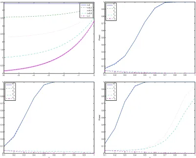
Figure 2 gives the plot for the drift function at different weights and the power curves
for all the tests under the three sample sizes considered. It is observed that all the tests
exhibit higher power when the sample size increases. For the density based tests, the
model-free test and the originalL2 type test seems to have almost identical power; while for the return based tests, the model-free test T4 seems more powerful than the original test T3. When the sample size is small, the return density based tests outperform the volatility density based tests when the deviation is large (when τ > 0.5). When the
sample size is large, the volatility density based test seems to be more powerful than the return based tests, except when the deviation to the null model is large (when τ >0.9).
6.2.2 Misspecification in the diffusion function
In this sequence of alternative models, the drift function remains the same, but the
diffusion function is deviating away from a constant:
d lnσ2t =α(β−lnσ2t)dt+{(1−τ)γ+τ ρ(σt2)}dWt (11)
Figure 4 gives the plot for the diffusion function at different weights and the power
curves for all the tests under the three sample sizes. The volatility density based tests
strictly dominate the return based tests in the scenarios considered; the return density
based tests seem to be sensitive to the sample size, it starts to get power only when the
sample size is large (15 years data), the Cramer von Mises test seem to have no power
for this type of alternative models, at least for the sample size used in the simulation.
To better understand the power for different tests under the two sequences of
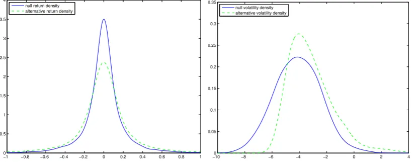
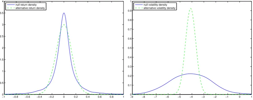
alter-native models, the return density and volatility density are plotted under both the null
hypothesis and the alternative hypothesis for the two types of alternative models in
Fig-ure 3 and 5. In FigFig-ure 3, the nonlinear deviation in the drift function cause both visible changes in the volatility density and the return density. In Figure 5 however, it is noticed
that the deviation in the diffusion function cause big change in the volatility density, but
only a small change in the variance of the return density. This perhaps explains why the
volatility density based tests performs much better than the return density based tests
for the deviations in the diffusion function.
[Figure 2 about here.]
[Figure 3 about here.]
[Figure 4 about here.]
[Figure 5 about here.]
7
Empirical example
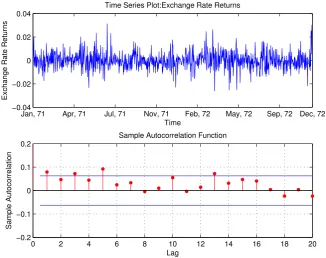
In this section, the tests developed in this paper are applied to a daily British pound/Canadian
dollar exchange rate dataset from January 1971 to August 1996. This dataset was used to estimate a discrete-time SARV model in Van der Sluis (1997). Figure 6 provides a
plot of the exchange rate returns and the sample AutoCorrelation Function (ACF) of the
squared returns, from which volatility clustering is observed.
The following continuous-time Log SARV model (9) is estimated with this dataset
using the GMM estimator of Meddahi (2002):
dYt =σtdWt,
d lnσt2 = 26.8630(−4.4991−lnσt2)dt+ 3.0999dBt,
where the parameter values are annualized. The parameter values are very close to those
implied by the discrete-time model estimated by Van der Sluis (1997).
a bandwidth 0.28. Based on 1000 bootstrap samples, the p-values of all the tests are
estimated. The p-values of all these tests are reported in the following table. All the
tests show strong evidence of rejection of the null model, other than the Cramer von
Mises test T5, which can only reject the model if the significance level 0.1 is used.
[Figure 6 about here.]
[Table 2 about here.]
8
Conclusion
This paper studies volatility density based nonparametric specification tests for
stochas-tic volatility models. The asymptostochas-tic null distributions of the test statisstochas-tics and their
asymptotic power properties are derived. A parametric bootstrap procedure is proposed
to obtain the null distributions and the critical values. The finite sample properties of
the method are studied using Monte Carlo simulations. The tests are applied to a simple
empirical application.
With high-frequency data, alternative test statistics could be proposed. For example,
using the methods developed in Kanaya and Kristensen (2015), nonparametric estimates of the drift and diffusion functions of the volatility process could be obtained, and test
statistics could be formulated based on these functions. This approach of
construct-ing tests will provide opportunities to test the original null hypothesis H0 against the alternative hypothesis H1 directly.
Appendix A: Assumptions and probability properties
of the stochastic volatility models
In this Appendix, the basic setup and the assumptions of the model (1) are established.
These assumptions are made for the observed return sequence to be stationary, ergodic
andβ-mixing with exponentially decaying coefficients, which are necessary for the limiting
theorems to work. In the nonparametric model, it is sufficient to assume the observed
return sequence{yti}ni=1to satisfy the above conditions directly. In the parametric model, assumptions are imposed on the b(x;θ) and a(x;θ) functions.
In the parametric stochastic volatility model (1), it is assumed that
(SV0) (B, W) is a standard Brownian motion in R2, defined on the probability space (Ω,F,P), and σ2
(SV1) The functionsb(x;θ) anda(x;θ) are continuous function onR+, and continuously differentiable functions on (0,+∞) such that
∃C > 0, ∀x >0, b2(x;θ) +a2(x;θ)6C(1 +x2),
and
∀x >0, a(x;θ)>0.
Now define, forv0 >0, the scale measure
s(x;θ) = exp
−2
Z x
v0
b(v;θ) a2(v;θ)du
,
and the speed measure
m(x;θ) = 1
a2(x;θ)s(x;θ), and assume
(SV2)
Z u
0
s(x;θ)dx= +∞,
Z +∞
v
s(x;θ)dx= +∞,
Z +∞
0
m(x;θ)dx=M <+∞,
where u >0, v <+∞ are arbitrary points in the domain of s(x;θ).
(SV3) The initial random variable σ2
0 has distribution π(dx) =π(x;θ)dx. (SV4)
lim
x↓0 a(x;θ)m(x;θ) = 0, xlim↑+∞a(x;θ)m(x;θ) = 0.
(SV5) Define
γ(x;θ) =a0(x;θ)−2b(x;θ)
a(x;θ),
then asx↓0 and x↑+∞, the limit of 1/γ(x;θ) exist.
(SV0) rules out the possibility of so called leverage effects. (SV1) ensures the existence
and uniqueness of a almost surely positive strong solution to the volatility process. (SV2)
implies the solution is positive recurrent on (0,+∞) (positive recurrent is also called
ergodic). The last condition in (SV2) guarantees the existence of a stationary distribution
for the volatility process, with density defined as
π(x;θ) = m(x;θ)
M I{x >0}. (12)
So if the process is initiated from this stationary distribution as in (SV3), the volatility
the volatility process is β-mixing. These conditions are standard for diffusion processes,
see Genon-Catalot et al. (1998) and Chen et al. (2010) for a detailed discussion. (SV4)
and (SV5) (together with (SV1) and (SV2)) are actually sufficient conditions for the
volatility process to be ρ-mixing. From Theorem 3.6 in Chen et al. (2010), a sufficient
condition (together with (SV1) and (SV2)) for exponential decayβ-mixing coefficients is
the process to beρ-mixing — this is not a very strong assumption, because as discussed
in the same paper, β-mixing and ρ-mixing with exponential decay are almost equivalent
concepts for a scalar diffusion. It is also a known result that if a diffusion process is
ρ-mixing, itsρ-mixing coefficients decay at exponential rate (Bradley (2005), theorem 3.3,
or Genon-Catalot et al. (2000), proposition 2.5). So with (SV4) and (SV5), the volatility process is β-mixing with exponentially decaying coefficients.
The exponential rate decay of the β-mixing coefficients for the observed returns is a
sufficient condition to use the limiting theorem for U-statistics; it could be reduced to
a polynomial rate if only for the purpose of applying the limiting theorem. However,
establishing sufficient conditions for the volatility process in the parametric model to be
β-mixing with a polynomial rate is not straightforward. In this sense, the exponential
rate decay of theβ-mixing coefficients should not be understood as a strong assumption.
The conditions above only deliver properties for the volatility process, the following
lemma shows that the return sequence yi =
Rti
ti−1σsdBs/
√
∆, i = 1, . . . , n, which is a sequence of stochastic integrals of the volatility process with respect to an independent
Brownian motionB over small fixed intervals, inherits the probabilistic properties of the
volatility process.
Lemma 1 In model (1), if the volatility process is stationary, ergodic andβ mixing with a
certain decay rate, then the normalized return sequenceyi, i= 1, . . . , n, is also stationary,
ergodic and β mixing with coefficients decaying at least as fast as that of the volatility.
Proof Using Theorem 3.1 in Genon-Catalot et al. (2000). (yi)ni=1 satisfy a Hidden Markov model with hidden chainUi := (
Rti
ti−1σ
2
sds, σ2ti),i= 1, . . . , n, thus also a
General-ized Hidden Markov Model as in the definition in Carrasco and Chen (2002). Applying
the proposition 4 in the latter paper, the return series (yi)ni=1 is ergodic, strictly stationary and β-mixing with at least the rate in the Hidden chainUi,i= 1, . . . , n. As noted in the
proof of proposition 3.2 in Genon-Catalot et al. (2000),
βU(k)6βσ2((k−1)∆),
meaning that the decay of the β-mixing coefficient of (Ui)ni=1 is at least as fast as that of (σ2
ti)ni=1, which completes the proof.
(C1) g(x) is first differentiable, g(x) and its derivative are bounded and square
inte-grable. f(x) is Lipschitz and bounded. Also assume the density of all the finite
dimensional distributions of the observed returns to be bounded.
(B1) Under the null hypothesis, the parametric estimator is √n-consistent for the true parameter value.
(B1a) Under both the alternative hypotheses H0
1 and H
0
1n, the parametric estimator is √
n-consistent for a pseudo-true value.
(B2) g(x, θ) is Lipschitz in the parameter θ, with the Lipschitz constant L(x) to be
square integrable.
Appendix B: Proofs of the theorems
Proof (of Theorem 1) The derivation of Theorem 1 is closely related to the derivation of
the asymptotic normality of the Integrated Squared Error (ISE) of the kernel
deconvolu-tion estimator. For independent and identically distributed observadeconvolu-tions, the asymptotic
distributions of ISE for different classes of signal densities and noise distributions were
derived by Butucea (2004). The result in Theorem 1 extends the corresponding results
of Theorem 4 in Butucea (2004) to dependent observations.
First the estimator can be written as
ˆ
g(x) = 1 n
n X
i=1 1 hνh
x−Yi
h
= 1 n
n X
i=1
ωh(x−Yi),
where ωh is defined implicitly.
Notice that
T0 =
Z 1
n
n X
i=1
ωh(x−Yi)−g(x; ˆθ)
!2
dx
=
Z 1
n
n X
i=1
ωh(x−Yi)−Kh∗g(x) +Kh∗g(x)−g(x) +g(x)−g(x; ˆθ)
!2
dx
= T1+
Z
(Kh∗g(x)−g(x))2dx+
Z
g(x)−g(x; ˆθ)2dx
+2
Z 1
n
n X
i=1
ωh(x−Yi)−Kh∗g(x) !
(Kh∗g(x)−g(x)) dx
+2
Z
1 n
n X
i=1
ωh(x−Yi)−Kh∗g(x) !
g(x)−g(x; ˆθ)dx
+2
Z
(Kh∗g(x)−g(x))
whereT1 is the bias-corrected statistic defined in Section 4.1. It will be shown later that T1 =Op(exp(π/h)/n). Notice that the integrated squared bias
R
(Kh ∗g(x)−g(x))2dx=
Op(h2) because of Assumption C1 and the “infinite order kernel” property of the sinc
ker-nel (see e.g. Theorem 8.1 of Glad et al. (2007));R
g(x)−g(x; ˆθ)2dx=Op(n−1) follows
from Assumption B2; so both terms are dominated by T1 under the bandwidth assump-tion. The cross product terms are also dominated by T1 because of the Cauchy-Schwarz inequality. One then has T0 = T1(1 +op(1)). Next the asymptotic distribution of T1 is derived.
First T1 is decomposed as follows,
T1 =
Z 1
n
n X
i=1
ωh(x−Yi)−Kh∗g(x)
!2
dx
= 1
n2
n X
i=1
Z
(ωh(x−Yi)−Kh∗g(x))2dx
+2 n2
X
16i<j6n Z
(ωh(x−Yi)−Kh∗g(x)) (ωh(x−Yj)−Kh∗g(x)) dx
=: S1+S2,
where S1 and S2 are defined implicitly. It is shown that
1. exp(24ππ/h2n)2kfk2 2
1/2
|S1−ES1|=op(1), where ES1 = (1/(2π2n)) exp(π/h).
2. exp(24ππ/h2n)2kfk2 2
1/2
S2
d −
→N(0,1).
3. Then it is proved that
4π2n2 exp(2π/h)kfk2
2
1/2
(T1−ES1)
d −
→N(0,1),
by combining the above two results. This also derives the asymptotic distribution
1. Order of S1 The order of E(S1) is first evaluated. By stationarity,
ES1 = 1 nE
Z
(ωh(x−Y1)−Kh ∗g(x))2dx
= 1
n
Z
E ωh2(x−Y1)−2ωh(x−y1)Kh∗g(x) + (Kh∗g(x))
2
dx
= 1
n
Z
E(ωh(x−Y1))2dx−
Z
(Kh∗g(x))2dx
= 1
n
Z Z 1
h2ν 2
h
x−Y1 h
f(y1)dy1dx−
Z
(Kh∗g(x))2dx
= 1
n
Z Z 1
hν 2
h(z)f(x−zh)dzdx− Z
(Kh∗g(x))2dx
= 1
n
Z Z 1
hν 2
h(z)f(x)dzdx(1 +o(1))− Z
(Kh∗g(x))2dx
= 1
nhkνhk 2
2(1 +o(1))− 1 n
Z
(Kh ∗g(x))
2 dx,
where in the third step Eωh(x−Y1) =Kh∗g(x) (see e.g. Stefanski and Carroll (1990))
is used, in the fifth step a change of variable using z = (x−y1)/h is applied and in the sixth step the Lipschitz assumption for f(x) is used.
Use Lemma 3, it can be calculated that the first term is (1/(2π2n)) exp(π/h); the sec-ond term is O(1/n) by noticing that R (Kh∗g(x))
2
dx= (1/(2π))R |φK(th)∗φg(t)|2dt≤
(1/(2π))R |φg(t)|2dt and that g(x) is square integrable; so the first term is dominating
and it is shown that
ES1 = (1/(2π2n)) exp(π/h). (13)
Then the order of the variance of V ar(S1) is evaluated.
Var(S1)
= 1 n4
n X
i=1
Var
Z
(ωh(x−Yi)−Kh∗g(x))2dx
+
2 n4
n−1
X
i=1
(n−i)Cov
Z
(ωh(x−Y1)−Kh∗g(x))2dx, Z
(ωh(x−Yi+1)−Kh∗g(x))2dx
For the diagonal terms, it is noticed that
Var
Z
(ωh(x−Yi)−Kh∗g(x))
2 dx
≤ E
Z
(ωh(x−Yi)−Kh∗g(x))
2 dx
2
= E
Z
(ωh(x−Yi))
2 dx
2
(1 +o(1))
= 1
h2kνhk 4
2(1 +o(1)), (15)
where a similar strategy in deriving the order for ES1 is used. For the covariance term, notice that
Cov
Z
(ωh(x−Y1)−Kh∗g(x))
2 dx,
Z
(ωh(x−Yi+1)−Kh∗g(x))
2 dx
≤ β(i)δ/(1+δ)E
Z
(ωh(x−Yi)−Kh∗g(x))2dx
1+δ!1/(1+δ)
= β(i)δ/(1+δ)1 hkνhk
2
2(1 +o(1)) (16)
for δ >0, where Lemma 1 of Yoshihara (1976) is used.
Plug the results (15) and (16) back into (14), one can obtain that
Var(S1)
= 1
n3h2kνhk 4
2(1 +o(1)) + 2 n3hkνhk
2 2
n−1
X
i=1
1− i
n
β(i)(δ−2)/δ(1 +o(1))
≤ C
n3h2kνhk 4
2(1 +o(1)),
for a large constant C > 0 because Pni=1−1 1− i n
β(i)(δ−2)/δ = O(1) by the exponential
rate of decay for the β-mixing coefficients. Use Lemma 3, it is obtained that
Var(S1) =O
1 n3 exp(
2π h )
. (17)
Combine the results in (13) and (17), and use the Markov’s inequality one has
S1 =Op
exp(π/h) n
and
(S1−ES1) =Op
exp(π/h) n3/2
Limiting distribution of S2 Recall that
S2 = 2 n2
X
16i<j6n Z
(ωh(x−Yi)−Kh ∗g(x)) (ωh(x−Yj)−Kh∗g(x)) dx
This is a U-statistic with kernel function
Hn(x, y) =
2 n2
Z
(ωh(u−x)−Kh∗g(u)) (ωh(u−y)−Kh∗g(u)) du.
It is easy to see this is a symmetric kernel, and
EHn(Yi, x) = 0,
∀x ∈ R. Now the central limit theorem from Hjellvik et al. (1998) is applied to derive the limiting distribution of S2.3
First, the asymptotic varianceσ2
nis calculated. This is done by calculating the
asymp-totically equivalent quantity n2σ02/2, where σ20 =R Hn2(Y1, Y2)dP(Y1)dP(Y2). Define the notation ξh(x) =
R
νh(x+z)νh(z)dz, one has:
σ02
= 4
n4
Z Z Z
(ωh(u−y1)−Kh∗g(u)) (ωh(u−y2)−Kh∗g(u)) du
2
f(y1)f(y2)dy1dy2
= 4
n4
Z Z Z
ωh(u−y1)ωh(u−y2)du
2
f(y1)f(y2)dy1dy2(1 +o(1))
= 4
n4h4
Z Z Z
νh
u−y1
h
νh
u−y2
h
du
2
f(y1)f(y2)dy1dy2
= 4
n4h2
Z Z
ξh2
y1−y2
h
f(y1)f(y2)dy1dy2
= 4
n4h
Z
ξh2(x) dx× kfk2 2+o
Z
ξh2(x) dx
.
The last approximation above is valid because for an arbitrarily small ε >0, ε →0 and
3Notice that the assumptionE[H
n(Yi, Yj)|Fj−1] = 0, for anyi < j does not hold apparently, but as
ε/h→ ∞ when n→ ∞, the following holds: Z Z 1 hξ 2 h
y1 −y2 h
f(y1)f(y2)dy1dy2−
Z
ξh2(x) dx× kfk22 = Z Z
ξh2(u)f(uh+y2)f(y2)dudy2−
Z
ξ2h(x) dx
Z
f2(x)dx
= Z Z
ξh2(u) (f(uh+y2)−f(y2))f(y2)dudy2
6 Z Z
ξh2(u)|f(uh+y2)−f(y2)|f(y2)dudy2
=
Z Z
|uh|6ε
ξh2(u)|f(uh+y2)−f(y2)|f(y2)dudy2
+
Z Z
|uh|>ε
ξ2h(u)|f(uh+y2)−f(y2)|f(y2)dudy2
6
Z Z
|uh|6ε
ξh2(u)f(y2)dudy2εL
+
Z Z
|uh|>ε
ξ2h(u)f(y2)dudy2×2 sup
f
kfk∞
6 o
Z
ξh2(x) dx
+o(1),
where in the fifth step the Lipschitz and boundedness assumptions for f(x) are used.
Using Lemma 3, one has
σn2 ∼ n
2 2 σ
2 0 =
1 4π2n2exp
2π h
× kfk22×(1 +o(1)). (18)
Next, upper bounds for Min for i= 1, . . . ,6 are evaluated. Basically, these are terms
of the form,
HijHkl = Hn(Yi, Yj)Hn(Yk, Yl)
= 4
n4
Z
(ωh(u−Yi)−Kh∗g(u)) (ωh(u−Yj)−Kh ∗g(u)) du
× Z
(ωh(u−Yk)−Kh∗g(u)) (ωh(u−Yl)−Kh∗g(u)) du
= 4
n4
Z
ωh(u−Yi)ωh(u−Yj)du Z
ωh(u−Yk)ωh(u−Yl)du(1 +o(1)),
I start with the quantity Mn2.
E|H1jHij|2(1+δ)
=
1 n4h2
2(1+δ)
E
ξh
Y1−Yj
h
ξh
Yi−Yj
h
2(1+δ)
=
1 n4h2
2(1+δ)Z Z Z
ξh
y1 −yj
h
ξh
yi−yj
h
2(1+δ)
f(y1, yi, yj)dy1dyidyj
=
1 n4h2
2(1+δ)
h2
Z Z Z
|ξh(z)ξh(z0)|2(1+δ)f(yj+zh, yj +z0h, yj)dzdz0dyj
6 C
1 n4h2
2(1+δ)
h2kξhk4(1+2(1+δδ)),
where in the last step the integrability for the joint density function is used andC > 0 is
a generic large constant. With the same method, it can be shown that other quantities in
the definition ofMn2 share this same upper bound, such that this is also an upper bound for their maximum Mn2. Use Lemma 3, one has
n3/2M
1 2(1+δ)
n2 σ2
n
=O(n−1/2) =o(1),
for δ >0.
Using the same strategy it can be shown that
E|H1jHij|2 6 C
1 n4h2
2
h2kξhk42,
E|H1iHjk|2(1+δ) 6 C
1 n4h2
2(1+δ)
h2kξhk
4(1+δ) 2(1+δ),
where C >0 is a generic large constant. Such that n3/2M1/2
n3 /σ2n =O(n−1/2) = o(1) and
For Mn5, notice that E Z
H1iH1jdP(Y1)
2(1+δ)
= E 4 n4h2
Z
ξh
y1−Yi
h
ξh
y1−Yj
h
f(y1)dy1
2(1+δ)
(1 +o(1))
=
1 n4h
2(1+δ)Z Z
Z
ξh(z)ξh
z+yi−yj h
f(zh+yi)dz
2(1+δ)
f(yi, yj) dyidyj(1 +o(1))
6 C
1 n4h
2(1+δ)Z Z Z
ξh(z)ξh
z+yi−yj h
2(1+δ)
f(zh+yi)dzf(yi, yj) dyidyj
= C
1 n4h
2(1+δ)
h
Z Z Z
|ξh(z)ξh(z+u)|2(1+δ)f(zh+yi)dzf(yi, yi−uh) dyidu
6 C
1 n4h
2(1+δ)
h
Z
|ξh(z)|2(1+δ)dz
2
= C
1 n4h
2(1+δ)
hkξhk
4(1+δ) 2(1+δ),
where C > 0 is a generic large constant. In the third step the Jensen’s inequality is
used, in the fifth step the integrability of the joint density function of observed returns
is used. With the same argument, the other quantities in the definition of Mn5 also have this upper bound, so Mn5 has this upper bound. Still use the result of Lemma 3, it is obtained that
n2M
1 2(1+δ)
n5 σ2
n
=O(h1−2(1+1δ)) = o(1),
for δ >0. In the same fashion, it can be shown that
E Z
H1iH1jdP(Y1)
2
6C6n−8h−1kξh(x)k
4 2,
and
n2M12
n6 σ2
n
=O(h1/2) =o(1).