Novel Fault Location in MTDC Grids with
Non-Homogeneous Transmission Lines Utilizing
Distributed Current Sensing Technology
Dimitrios Tzelepis,
Member, IEEE,
Grzegorz Fusiek,
Member, IEEE,
Adam Dy´sko,
Member, IEEE,
Pawel
Niewczas,
Member, IEEE,
Campbell Booth, and Xinzhou Dong,
Fellow, IEEE,
Abstract—This paper presents a new method for locating faults in multi-terminal direct current (MTDC) networks incorporat-ing hybrid transmission media (HTMs), includincorporat-ing segments of underground cables (UGCs) and overhead lines (OHLs). The proposed travelling wave (TW) type method uses continuous wavelet transform (CWT) applied to a series of line current measurements obtained from a network of distributed optical sensors. The technical feasibility of optically-based DC current measurement is evaluated through laboratory experiments using Fiber-Bragg Grating (FBG) sensors and other commercially available equipment. Simulation-based analysis has been used to assess the proposed technique under a variety of fault types and locations within an MTDC network. The proposed fault location scheme has been found to successfully identify the faulted segment of the transmission media as well as accurately esti-mating the fault position within the faulted segment. Systematic evaluation of the method is presented considering a wide range of fault resistances, mother wavelets, scaling factors and noisy inputs. Additionally, the principle of the proposed fault location scheme has been practically validated by applying a series of laboratory test sets.
Index Terms—Fault Location, Multi Terminal Direct Current, Travelling Waves, Wavelet Transform, Distributed Optical Sens-ing
I. INTRODUCTION
W
ITH recent rapid development of power electronics, high voltage direct current (HVDC) networks incor-porating voltage source converters (VSCs) have become an attractive option for bulk power transfer from offshore wind farms [1], [2] and also for upgrading and interconnecting existing AC systems [3], [4].When a permanent fault occurs in an HVDC transmission system, accurate estimation of its location is of major impor-tance in order to accelerate restoration, minimize repair cost, and thus reduce the system down-time.
This paper deals with the challenges related to accurate fault location in HVDC networks with non-homogeneous transmission media including segments of UGCs and OHLs. The remainder of the paper is organized as follows: Section
The present article outlines the results of a collaborative work conducted between University of Strathclyde, Glasgow, UK and Tsinghua University, Beijing, China. This work was supported in part by GE Solutions Ltd, the Innovate UK (TSB Project Number 102594), the European Metrology Research Programme (EMRP) - ENG61, the Natural Science Foundation of China (Grant No. 51120175001) and the National Key Research and Development Plan of China (Grant No. 2016YFB0900600). The EMRP is jointly funded by the EMRP participating countries within EURAMET and the European Union.
II presents a review of existing fault location techniques for HVDC networks. In Section III, the proposed fault location method is explained. The case studies and simulation results are presented in Section IV. The optical sensing technology together with the experimental setup are introduced in Section V. Finally, in Section VI conclusions are drawn.
II. FAULTLOCATION INHVDC SYSTEMS
It has been demonstrated in many publications that travel-ling waves (TW) can be used to accurately estimate fault po-sition on a transmission line. This estimation can be achieved using measurements either from a single end or from both ends of the faulted circuit. Single-ended methods require iden-tification of two consecutive TW reflections measured at one terminal, while the two-ended methods use the first reflection only (captured and time-stamped at both line terminals). As the first reflection always provides the clearest signature, two-ended methods are considered more reliable [5]. Nevertheless, the selection between single-ended and two-ended methods is a trade-off between the cost, complexity and required reliability of the estimation [6].
Even though capable of providing high accuracy estima-tions, TW-based fault location comes with a number of challenges such as difficulty of wavefront detection, high dependency on sampling frequency, requirement for very accurate sampling synchronization (for two-ended methods), and uncertainties in estimation of propagation velocity in the transmission media.
A wavelet transform (WT) approach is utilized in [7] to locate the faults in star connected MTDC systems. The method uses continuous wavelet transform (CWT) applied to the DC line current waveforms, and is shown to be capable of completely eliminating the requirement for repeater stations at the network junctions. However, a high sampling frequency (2 MHz) and time synchronized measurements are required. Additionally, high impedance faults have not been investigated thoroughly.
both publications [8], [9], indicate a need for high sampling frequency of 1 MHz.
A special category of fault location (which is the main focus of this paper) applies to networks which include hybrid feeders with segments of both UGC and OHL. It should be emphasized that in such networks, additional challenges for TW-based methods arise from the fact that the speed of electromagnetic wave propagation is not uniform, additional reflections are generated at the junction points, and there is an increased difficulty in identifying the faulted segment. For such networks in HVDC systems, a number of fault location approaches are presented in [5], [10].
The authors of [5] propose the application of two-ended TW-based fault location based on time-stamped measurements (voltages and capacitor currents) sampled at 2 MHz. Prior to the TW-based fault location, the faulted segment is found by solving a set of equations estimating distance to fault for each segment. The method is very accurate even with noisy inputs, however fault resistances up to 100 Ω were only taken into account. Additionally, the requirement of high sampling rate and synchronized measurements could be considered a barrier in practical applications.
An alternative approach is presented in [10] where a support vector machine (SVM) is used for faulted segment identifica-tion, while an analysis based on TWs estimates the location of the fault. The method is single-ended and requires both current and voltage measurements. However, the presented case studies consider fault resistances only up to 70Ω, while the sampling frequency requirements are not clearly stated. Additionally, the proposed SVM-based learning algorithm can incorporate two classes of lines only, which means that the proposed algorithm can only be applied to networks with two different segments.
III. PROPOSEDFAULTLOCATIONSCHEME
The fault location scheme presented in this paper utilizes the TW principle applied to a series of measured waveforms obtained from current sensors distributed along the transmis-sion line. The distributed optical measuring arrangement has been previously shown by the authors as being capable of enabling highly discriminative DC line protection. The details and rationale for utilizing distributed optical sensing can be found in [11]. It should be noted here that the key advantage of the measuring arrangement is that all sensing points are completely passive (i.e. require no power supply) and can be interrogated directly from a single piece of equipment at either end of the line, where the protective equipment is placed. In fault location applications, the immediate benefit of multiple distributed sensing is that the fault location can be successfully performed in transmission lines containing multiple segments, and is not limited to two segments as described in [10]. Additionally, when compared to [5] and several other methods, the proposed fault location approach requires neither high sampling frequency nor accurate time-stamping (i.e. GPS).
As the scheme depends primarily on the utilization of TWs which can be observed in both voltage and current waveforms, the choice of specific signal is usually guided by the ease of
measurement and cost. In this case, the current was considered more appropriate due to the availability of the distributed optical sensing arrangement used previously in the current-based protection described in [11]. However, in a different practical situation the use of voltage measurement could also provide similar fault location functionality.
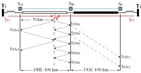
[image:2.612.316.558.220.394.2]The proposed fault location scheme consists of three main stages as depicted in Fig. 1. Those are explained in detail in the following subsections. To enhance clarity of the description an example illustration is presented in Fig. 2 which includes a hybrid circuit with 100 km OHL and 100 km UGC. A fault is shown to occur on the OHL at a distance of 70 km from T1 (where the measurements are collected).
Fig. 1. Fault location algorithm flow chart.
A. Stage I: Faulted Segment Identification
In this stage the faulted segment (e.g. UGC or OHL) is identified. As seen in Fig. 1, prior to any processing the measurements are compensated for the time delay imposed by the optical fiber. Such time delay corresponds to the speed of light and the refractive index of SMF-28 fiber which can be found in [12]. The fault segment identification approach is illustrated in more detail in Fig. 4.
Fig. 2. Bewley Lattice diagram incorporating OHL, UGC and distributed optical current sensors.
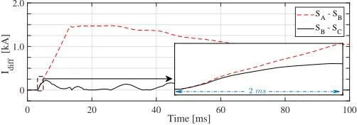
[image:2.612.315.563.558.687.2]sensors. When a fault occurs between two sensors, the differ-ential current derived from those sensors reaches much higher level than the current derived from any other adjacent pair. For the fault case shown in Fig. 2 differential current Idif f is calculated for the two adjacent sensor pairs SA−SB and
SB−SC, and is illustrated in Fig. 3. The difference is almost one order of magnitude which allows for a reliable selection of the faulted section of the line using a simple instantaneous value comparison.
0 20 40 60 80 100
Time [ms]
0 1.0 2.0
I diff
[kA]
S A - SB S
[image:3.612.313.563.111.198.2]B - SC
Fig. 3. Differential currents for the fault case corresponding to Fig. 2.
The identification stage produces two outputsSU PandSDN which correspond to the two adjacent sensors, one upstream and one downstream with respect to the fault (SA andSB in the depicted case). To achieve this, the algorithm incrementally searches for the first sensor (index r) corresponding to the highest differential current (in this case r =A). This sensor becomes SU P =r, and the adjacent sensor becomesSDN=
[image:3.612.49.300.179.267.2]r+ 1 (considering that highest differential current has been reached by measurements of sensors randr+ 1).
Fig. 4. Faulted segment identification algorithm.
Since high frequency components are not used at this stage (and also to eliminate any interference from noise), a moving average with a time window of 5 ms is applied. It is also shown in the zoomed area of Fig. 3 that only a small amount of post-fault data (less than 1 ms) is needed to successfully perform the faulted segment identification. This is evident from the zoomed area of the initial 2.0 ms following the fault where the current corresponding to the faulted segment can be clearly distinguished from a very early stage. Consequently, the performance of the proposed faulted segment identification cannot be jeopardized, even with ultra fast DC protection schemes (considering combined detection and isolation time). It should be emphasized that the proposed scheme can identify the faulted segment regardless the position of the fault (i.e. OHL or UGC) or the number of series-connected segments combined into one feeder. This is extensively demonstrated in Section IV-C.
B. Stage II: Wave Detection
In this stage the precise time of wave arrival is established. The algorithm initiates with the selection of the two
mea-surements adjacent to the faultSU P andSDN as reported by Stage I. Those measurements are then processed by the CWT to detect the precise arrival times of the individual TWs.
0 0.5 1 1.5
Time [ms]
0 0.2 0.4 0.6 0.8 1 1.2
CWT magnitude SA SB SC
t1(SB) t1(SA) t 1(SC)
t 3(SB) t
2(SB) t
2(SA)
t3(SA) t2(SC)
Fig. 5. Normalized absolute values of wavelet coefficient magnitudes for the fault case corresponding to Fig. 2.
The wavelet transform of a function ζ(t)can be expressed as the integral of the product ofζ(t)and the daughter wavelet
Ψ∗a,b(t)as presented in equation (1).
Wψζ(t) =
Z ∞
−∞
ζ(t) √1
αΨ
t−b
a
| {z }
daughter waveletΨ∗ a,b(t)
dt (1)
The daughter waveletΨ∗a,b(t)is a scaled and shifted version of the mother wavelet Ψa,b(t). Scaling is implemented byα which is the binary dilation (also known as scaling factor) and shifted by bwhich is the binary position (also known as shifting or translation).
In Fig. 5 the normalized absolute values of wavelet coef-ficient magnitudes for the fault case corresponding to Fig. 2 are depicted. It should be noted that the magnitudes have been normalized individually according to the maximum value of the TWs in each measurement (which is usually the initial TW).
In this case the selected measurements would be from sensors SA (black solid line) and SB (green dashed line). The exact times of the waves are established by comparing the waveforms with a predefined thresholdWT H (i.e. the time instant is recorded when the threshold is exceeded). For sensor
SA those time instances correspond tot1(SA) andt2(SA) (as
shown in Fig. 5), while for the sensor SB those times are depicted as t1(SB),t2(SB),t3(SB),t4(SB)andt5(SB).
C. Stage III: Fault location calculation
In the final stage of the algorithm, the actual fault location is calculated. Since the measurements from both ends of the faulted segment are available locally, two-ended fault location approach can be conveniently applied. It is worth reiterating that the utilized optical sensing scheme can interrogate all sensors from a single acquisition point, and thus synchronized measurements can be ensured without the need of GPS (i.e. the difference in measurement time arrival from individual sensors is known and can be easily calculated). Taking as a reference the left-hand side (i.e. whereSU P is located) of the HTM the fault location can be estimated using equation (2).
DF =
Lseg−∆t(SU P−SDN)·vprop
[image:3.612.53.300.414.477.2]where DF is the distance between SU P sensor and the fault (calculated using the measurements of both sensorsSU P and SDN), Lseg is the total length of the faulted segment,
∆t(SU P−SDN) is the time difference of the initial TWs at
sensing locationsSU P andSDN, andvprop is the propagation velocity of the faulted segment. For the studies presented in this paper the propagation velocity has been calculated according to the conductor geometry of each segment.
IV. SIMULATIONRESULTS
A. MTDC Study Network
A model of a five-terminal HVDC grid illustrated in Fig. 6 has been developed in Matlab/SimulinkR for the purposes of
evaluating the proposed fault location method. The network architecture has been adopted from the Twenties Project case study on DC grids [13]. There are five modular multi-level converters (MMCs) in the network operating at±400 kV (in symmetric monopole configuration), current limiting induc-tors, and HTMs with OHLs and UGCs (both are represented by the distributed parameter line model). It should be noted that by adopting a meshed MTDC network (rather than point-to-point HVDC links), the proposed fault location scheme is further scrutinized under an extended variety of faults occurring on different types of hybrid feeders.
The line lengths of each HTM segment can be seen in Table II. The parameters used in modelling of the OHLs and UGCs can be found in Table III [14].
Fig. 6. MTDC case study grid.
A network of distributed current optical sensors is installed on all HTMs. The sensors are installed at each line end, and one at each junction. The main purpose of the junction sensor is to facilitate the faulted segment identification. Therefore,
there is no need for the installation of two sensors at both sides of the junction (unless there were more than two lines connected to the node) as the same current would be measured by both sensors. Each sensing network is terminated at one end of the HTM where the measuring and fault location equipment (i.e. fault locator station) is placed. As the method is single-ended by its nature, there is only one optical measurement interrogator, and one fault locator station required for each HTM. Therefore, in some converter stations (e.g. M M C3)
there is no measuring equipment, only the sensors attached to the end of the optical fiber. More details regarding the optical measuring equipment are included in Section V. The fault location results presented in the following sections are reported taking the fault locator station as a reference point.
The MMC models utilized in this paper are identical to those used in [11] and the parameters of the AC and DC network components are included in Table I.
TABLE I
DCANDAC NETWORKPARAMETERS
Parameter Value
AC voltage[VAC,L−L] 400 kV
AC frequency[fn] 50 Hz
AC short-circuit level[Ss.c] 40 GVA
DC voltage[VDC] 800 kV
DC line external inductance[LDC] 150 mH
MMC number of sub-modules per arm 400 MMC arm inductance[LDC] 0.1 p.u.
TABLE II
LENGTHS OFOHLS ANDUGCSINCLUDED INMTDC CASESTUDYGRID
HTM-1 UGC: 150 km, OHL: 70 km HTM-2 OHL: 100 km, UGC: 100 km
HTM-3 OHL-a: 65 km, UGC: 180 km, OHL-b: 35 km HTM-4 UGC: 50 km, OHL: 130 km
HTM-5 UGC: 30 km, OHL: 70 km
TABLE III
PARAMETERS OFUGCANDOHL
Parameter OHL UGC
Resistance [Ω/km] 0.015 0.0146 Inductance [mH/km] 0.96 0.158 Capacitance [µF /km] 0.012 0.275 Speed of propagation [km/s] 294,627.8 151,706.8
B. Case Studies and Methodology
Pole-to-pole faults (PPFs) and pole-to-ground faults (PGFs) have been simulated in all segments of the MTDC network, at varying distances and with various fault resistances (Rf) of up to 500Ω. The simulation of the MTDC system and DC-side faults has been carried out at 1 MHz (i.e. with 1µstimestep), while the fault location algorithm has been executed at 135 kHz. Additionally, test cases have been expanded to include a wide range of mother wavelets Ψ, scaling factors α and the impact of noisy measurements.
the CWT magnitudes have been normalized (as also shown in Fig. 5). The threshold WT H used for establishing the wave arrival time has been set to 0.25. As also discussed in [7] the value of the threshold is subject to the assumed safety margins, anticipated levels of noise in the measured signal and scale of CWT.
The most suitable mother wavelet is usually selected by trial-and-error studies. The two major criteria are the provision of sharp edge for wave detection and the requirement for processing resources. However the latter is not so crucial in fault location applications as they are more focused on accuracy. For HVDC fault location applications it has been found in the literature that mother wavelets with relatively good performance include the ‘Haar’and‘db1’ [5], [7], [10] wavelets. This will be also verified in the next subsections with the aid of simulations.
The values of fault location estimation error have been calculated according to equation (3).
error [%] = DF−A.DF Lseg
·100% (3)
where DF is the calculated fault distance, A.DF is the actual fault distance and Lseg the total length of the faulted segment.
C. Fault Location Results
The results of faulted segment identification and fault lo-cation are included in Table IV for PPFs and Tables V and VI for resistive PGFs with Rf = 100 Ω and Rf = 500 Ω respectively. The presented results were obtained by utilizing
‘Haar’ mother wavelet with a scaling factor α = 2, since (theoretically) results with increased accuracy are expected in lower scales. To facilitate easier evaluation of the large amount of presented results, a few common statistical indices, comprising minimum, maximum and average error values, are frequently reported though the paper.
The minimum, maximum and average errors observed for PPFs are 0%, 1.4817% and 0.3768% respectively while for PGFs (Rf = 100 Ω) those errors were 0.0262%, 1.3389% and0.3714%respectively. The aforementioned errors for PGFs with Rf = 500 Ω correspond to 0.000%, 1.4770% and
0.4170% which verify that the proposed scheme is accurate even for highly-resistive faults. By observing 4th and 5th
column in Tables IV, V and VI it is evident that the faulted segment has been identified correctly in 100% of the cases for both types of faults. This has been achieved regardless the position of the fault (i.e. OHL or UGC) or the number of series-connected segments, which verifies the robustness of the proposed algorithm. What is also interesting to note is that the proposed fault location scheme achieves high accuracy even in the case of close-up faults (i.e. faults occurring close to the head or end of each line segment).
D. Effect of Mother WaveletΨand Scaling Factor α
In order to investigate the effect of mother wavelet Ψand scaling factorα, a section of UGC at HTM-3 has been tested. In particular, PPFs from 90 km to 120 km with steps of
TABLE IV
SEGMENTIDENTIFICATION ANDFAULTLOCATIONRESULTS FORPPFS
HTM Segment Fault Reported sensors Reported fault Error distance [km] SU P SDN location [km] [%] 1 UGC 25.0 S1−A S1−B 24.9929 -0.0047 1 UGC 55.0 S1−A S1−B 55.3343 0.2229 1 UGC 78.5 S1−A S1−B 78.3713 -0.0858 1 UGC 103.5 S1−A S1−B 103.6557 0.1038 1 UGC 141.0 S1−A S1−B 141.3015 0.2010 1 OHL 23.2 S1−B S1−C 22.9966 -0.2905 1 OHL 48.0 S1−B S1−C 48.2108 0.3012 1 OHL 57.7 S1−B S1−C 57.9155 0.3079 1 OHL 65.5 S1−B S1−C 64.4628 -1.4817 2 OHL 18.5 S2−A S2−B 18.3548 -0.1452 2 OHL 50.0 S2−A S2−B 51.0912 1.0912 2 OHL 63.6 S2−A S2−B 64.1858 0.5858 2 OHL 77.0 S2−A S2−B 77.2804 0.2804 2 UGC 9.0 S2−B S2−C 8.4211 -0.5789 2 UGC 43.8 S2−B S2−C 43.2575 -0.5425 2 UGC 69.4 S2−B S2−C 69.1038 -0.2962 2 UGC 88.0 S2−B S2−C 88.2076 0.2076 2 UGC 90.0 S2−B S2−C 89.8933 -0.1067 3 OHL-a 12.4 S3−A S3−B 11.7669 -0.9740 3 OHL-a 35.0 S3−A S3−B 35.7736 1.1902 3 OHL-a 42.0 S3−A S3−B 42.3209 0.4937 3 OHL-a 50.1 S3−B S3−C 51.0506 1.4625 3 OHL-a 57.3 S3−B S3−C 57.5979 0.4583 3 UGC 10.0 S3−B S3−C 9.6516 -0.1936 3 UGC 39.7 S3−B S3−C 39.9929 0.1627 3 UGC 56.7 S3−B S3−C 56.8493 0.0829 3 UGC 95.0 S3−B S3−C 95.0569 0.0316 3 UGC 100.0 S3−B S3−C 99.5519 -0.2489 3 UGC 103.0 S3−B S3−C 102.9232 -0.0427 3 UGC 161.2 S3−B S3−C 161.3584 0.0880 3 UGC 173.0 S3−C S3−D 172.5959 -0.2245 3 OHL-b 26.7 S3−C S3−D 26.6210 -0.2256 3 OHL-b 30.0 S3−C S3−D 29.9337 -0.1893 3 OHL-b 33.7 S3−C S3−D 33.8682 0.4806 4 UGC 3.8 S4−A S4−B 3.6487 -0.3027 4 UGC 13.2 S4−A S4−B 13.2006 0.0012 4 UGC 29.10 S4−A S4−B 29.4950 0.7900 4 UGC 46.6 S4−A S4−B 46.3513 -0.4973 4 OHL 29.0 S4−C S4−D 28.9899 -0.0077 4 OHL 53.5 S4−C S4−D 52.9966 -0.3872 4 OHL 74.0 S4−C S4−D 73.7297 -0.2079 4 OHL 110.2 S4−C S4−D 109.7398 -0.3540 4 OHL 125.0 S4−C S4−D 125.0168 0.0129 5 UGC 2.6 S5−A S4−B 2.6387 0.1290 5 UGC 7.9 S5−A S4−B 8.2575 1.1916 5 UGC 10.7 S5−A S4−B 10.5050 -0.6501 5 UGC 15.0 S5−A S4−B 15.0000 0.0000 5 UGC 29.5 S5−A S4−B 29.6088 0.3627 5 OHL 7.9 S5−B S4−C 7.7196 -0.2576 5 OHL 33.8 S5−B S4−C 33.9088 0.1554 5 OHL 45.5 S5−B S4−C 44.8209 -0.9701 5 OHL 66.6 S5−B S4−C 66.6452 0.0646 5 OHL 69.0 S5−B S4−C 68.8276 -0.2462
250 meters have been generated. For this range of faults the minimum (min), maximum (max) and average (avg) values have been calculated for different mother wavelets Ψ and scaling factors α, as shown in Table VII. The scaling factor values α have been selected using a power-of-two series
α= 2N (withN = 1,2, ..). This is a common practice adopted in WT [5], [7], [15], and it provides a common base for comparison between different methods but also for comparison between CWT and DWT (scaling factors in DWT can only assume values of the power of two).
Satisfactory results have been achieved for the majority of mother wavelets and scaling factors. However, an increase in fault location error can be observed when using the majority of mother wavelets with higher values of the scaling factor (e.g.
[image:5.612.316.559.82.504.2]TABLE V
SEGMENTIDENTIFICATION ANDFAULTLOCATIONRESULTS FORPGFS
(Rf = 100 Ω)
HTM Segment Fault Reported sensors Reported fault Error distance [km] SU P SDN location [km] [%] 1 UGC 39.5 S1−A S1−B 39.6017 0.0678 1 UGC 56.0 S1−A S1−B 55.8962 -0.0692 1 UGC 100 S1−A S1−B 100.2845 0.1896 1 UGC 135.6 S1−A S1−B 135.6827 0.0552 1 UGC 148.0 S1−A S1−B 148.0440 0.0294 1 OHL 12.2 S1−B S1−C 12.0845 -0.1650 1 OHL 38.7 S1−B S1−C 38.2736 -0.6091 1 OHL 43.2 S1−B S1−C 42.6385 -0.8021 1 OHL 68.0 S1−B S1−C 67.7364 -0.3765 2 OHL 19.8 S2−A S2−B 20.5372 0.7372 2 OHL 48.8 S2−A S2−B 48.9088 0.1088 2 OHL 88.8 S2−A S2−B 88.1925 -0.6075 2 OHL 90.0 S2−A S2−B 90.3749 0.3749 2 UGC 13.3 S2−B S2−C 12.9161 -0.3839 2 UGC 33.3 S2−B S2−C 33.1437 -0.1563 2 UGC 56.0 S2−B S2−C 55.6188 -0.3812 2 UGC 71.6 S2−B S2−C 71.3513 -0.2487 2 UGC 86.7 S2−B S2−C 87.0839 0.3839 3 OHL-a 7.9 S3−A S3−B 8.4933 0.9128 3 OHL-a 15.5 S3−A S3−B 16.1318 0.9720 3 OHL-a 38.9 S3−A S3−B 39.0473 0.2266 3 OHL-a 46.8 S3−A S3−B 46.6858 -0.1757 3 OHL-a 62.1 S3−A S3−B 61.9628 -0.2111 3 UGC 9.9 S3−B S3−C 9.6516 -0.1380 3 UGC 10.5 S3−B S3−C 10.7753 0.1530 3 UGC 59.0 S3−B S3−C 59.0968 0.0538 3 UGC 87.1 S3−B S3−C 87.1906 0.0503 3 UGC 100.0 S3−B S3−C 99.5519 -0.2489 3 UGC 144.0 S3−B S3−C 144.5021 0.2789 3 UGC 153.4 S3−B S3−C 153.4921 0.0512 3 UGC 166.0 S3−B S3−C 165.8534 -0.0814 3 UGC 177.7 S3−B S3−C 177.6528 -0.0262 3 OHL-b 20.5 S3−C S3−D 20.7736 0.7818 3 OHL-b 30.7 S3−C S3−D 30.5946 -0.3012 4 UGC 6.5 S4−A S4−B 6.4581 -0.0839 4 UGC 15.2 S4−A S4−B 15.4481 0.4962 4 UGC 25.5 S4−A S4−B 25.5619 0.1238 4 UGC 41.7 S4−A S4−B 41.8563 0.3126 4 OHL 10.8 S4−B S4−C 10.4393 -0.2775 4 OHL 55.3 S4−B S4−C 55.1791 -0.0930 4 OHL 65.4 S4−B S4−C 65.0000 -0.3077 4 OHL 99.1 S4−B S4−C 98.8276 -0.2095 4 OHL 115.4 S4−B S4−C 115.1959 -0.1570 5 UGC 5.2 S5−A S4−B 4.8862 -1.0460 5 UGC 6.6 S5−A S4−B 6.3344 -0.8854 5 UGC 14.7 S5−A S4−B 15.0000 1.0000 5 UGC 26.6 S5−A S4−B 26.2375 -1.2082 5 OHL 11.3 S5−B S4−C 10.9933 -0.4382 5 OHL 21.0 S5−B S4−C 20.8142 -0.2654 5 OHL 27.5 S5−B S4−C 27.3615 -0.1979 5 OHL 44.0 S5−B S4−C 44.4975 0.7107 5 OHL 58.0 S5−B S4−C 57.9155 -0.1207 5 OHL 65.4 S5−B S4−C 64.4628 -1.3389
‘db1’, ‘db2’, ‘sym1’ and ‘sym2’. The best overall accuracy in terms of average error has been achieved for mother wavelet‘coif2’and scaling factorα= 4. Predominantly, high performance is achieved to lower scales, as they correspond to higher frequency components and the accuracy is expected to be theoretically greater [5], [16].
E. Impact of Noisy Measurements.
In order to assess and further scrutinize the performance of the proposed fault location scheme, the studies presented in Section IV-D have been repeated considering noisy inputs. In particular, the current measurements have been subjected to artificial noise with increasing amplitude up to 28 dB Signal to Noise Ratio (SNR). Excessive noise may result at the transimpedance amplifier stage, particularly when spectral signals from Fiber Bragg Grating (FBG) sensors need to travel relatively long sections of optical fiber and require significant
TABLE VI
SEGMENTIDENTIFICATION ANDFAULTLOCATIONRESULTS FORPGFS
(Rf = 500 Ω)
HTM Segment Fault Reported sensors Reported fault Error distance [km] SU P SDN location [km] [%] 1 UGC 1.2 S1−A S1−B 1.3941 0.1294 1 UGC 5.7 S1−A S1−B 5.8891 0.1261 1 UGC 34 S1−A S1−B 33.983 -0.0114 1 UGC 100 S1−A S1−B 100.2845 0.1896 1 UGC 129 S1−A S1−B 129.5021 0.3347 1 UGC 149 S1−A S1−B 149.7297 0.4864 1 OHL 35 S1−B S1−C 35.0000 0.0000 1 OHL 55 S1−B S1−C 54.6419 -0.5116 1 OHL 67 S1−B S1−C 66.6452 -0.5068 2 OHL 1.5 S2−A S2−B 1.9866 0.4866 2 OHL 50.7 S2−A S2−B 51.0912 0.3912 2 OHL 90.2 S2−A S2−B 90.3749 0.1749 2 OHL 95 S2−A S2−B 94.7398 -0.2602 2 UGC 12.7 S2−B S2−C 12.3542 -0.3458 2 UGC 29.9 S2−B S2−C 29.2105 -0.6895 2 UGC 45.8 S2−B S2−C 44.9431 -0.8569 2 UGC 66.6 S2−B S2−C 66.2944 -0.3056 2 UGC 87.7 S2−B S2−C 87.6458 -0.0542 3 OHL-a 8.1 S3−A S3−B 8.4933 0.6051 3 OHL-a 23.8 S3−A S3−B 24.5979 1.2276 3 OHL-a 35.6 S3−A S3−B 35.7736 0.2671 3 OHL-a 46.5 S3−A S3−B 46.6858 0.2858 3 OHL-a 55.5 S3−A S3−B 55.4155 -0.1300 3 UGC 8.8 S3−B S3−C 8.5278 -0.1512 3 UGC 12 S3−B S3−C 11.8991 -0.0561 3 UGC 33 S3−B S3−C 33.2504 0.1391 3 UGC 56.4 S3−B S3−C 56.2874 -0.0626 3 UGC 100 S3−B S3−C 100.1138 0.0632 3 UGC 144.3 S3−B S3−C 144.5021 0.1123 3 UGC 156 S3−B S3−C 155.7396 -0.1447 3 UGC 165.7 S3−B S3−C 165.8534 0.0852 3 UGC 177.5 S3−B S3−C 177.6528 0.0849 3 OHL-b 15.2 S3−C S3−D 15.3176 0.3359 3 OHL-b 34 S3−C S3−D 33.8682 -0.3765 4 UGC 5.1 S4−A S4−B 5.3343 0.4686 4 UGC 28 S4−A S4−B 28.3713 0.7425 4 UGC 42 S4−A S4−B 42.4182 0.8364 4 UGC 48.5 S4−A S4−B 49.1607 1.3214 4 OHL 4 S4−B S4−C 2.8008 -0.9225 4 OHL 66 S4−B S4−C 66.0912 0.0702 4 OHL 83.5 S4−B S4−C 83.5506 0.0390 4 OHL 99 S4−B S4−C 98.8276 -0.1326 4 OHL 115.7 S4−B S4−C 116.2871 0.4516 5 UGC 2.7 S5−A S4−B 2.7056 0.0186 5 UGC 9.5 S5−A S4−B 9.9431 1.4770 5 UGC 11 S5−A S4−B 11.3287 1.0958 5 UGC 18.4 S5−A S4−B 18.6331 0.7771 5 UGC 28.5 S5−A S4−B 28.7469 0.8231 5 OHL 11.5 S5−B S4−C 10.9933 -0.7239 5 OHL 23 S5−B S4−C 22.9966 -0.0048 5 OHL 39.8 S5−B S4−C 39.3649 -0.6216 5 OHL 55.1 S5−B S4−C 54.6419 -0.6545 5 OHL 67.3 S5−B S4−C 66.6452 -0.9354
amplification. Due to space limitations only results for mother wavelet‘Haar’ are presented in Table VIII.
Compared to the noise-less signal (infinite SNR), the in-crease in noise level (lower dB values correspond to higher levels of noise) has inevitably a degrading effect on the fault location accuracy. It can be concluded that the proposed fault location scheme is relatively robust to the additive noise, symptomatic of the fiber section lengths and sampling rates (hence photodetector bandwidth) considered in this simulation. In terms of average error it has been found that the error rises by0.0369%for the SNR dropping to 28 dB.
F. Impact of Fault Current Limiters.
TABLE VII
FAULTLOCATIONERRORS OFPPFS ATUGC (HTM-3)FORDIFFERENTVALUES OFSCALINGFACTORαANDMOTHERWAVELETSΨ
PP
PP
PP
Ψ
α 2 4 8 16 32 64 128
min max avg min max avg min max avg min max avg min max avg min max avg min max avg
Haar 0.0000 0.2282 0.0860 0.0000 0.2667 0.0905 0.0000 0.2063 0.0833 0.0000 0.2448 0.0998 0.0000 0.5253 0.1505 0.0028 0.7055 0.3616 2.9111 4.4581 3.7014
db1 0.0000 0.2282 0.0860 0.0000 0.2667 0.0905 0.0000 0.2063 0.0833 0.0000 0.2448 0.0998 0.0000 0.5253 0.1505 0.0028 0.7055 0.3616 2.9111 4.4581 3.7014
db2 0.0000 0.2586 0.1102 0.0000 0.2517 0.0950 0.0000 0.1719 0.0788 0.0000 0.3906 0.1411 0.0014 0.6326 0.2840 0.7577 2.0462 1.1061 2.9303 3.5368 3.1106
db3 0.0000 0.7466 0.1285 0.0000 0.2229 0.0894 0.0000 0.4097 0.0958 0.0000 0.4097 0.0958 0.1472 0.9049 0.4186 1.0244 14.6712 1.8594 5.9309 17.3664 15.7722
db4 0.0000 0.4580 0.1357 0.0000 0.1719 0.0792 0.0000 0.2586 0.1081 0.0000 0.2420 0.0965 0.8073 7.0462 2.5598 2.1382 13.8035 6.9622 5.7920 19.4827 14.6758
sym1 0.0000 0.2282 0.0860 0.0000 0.2667 0.0905 0.0000 0.2063 0.0833 0.0000 0.2448 0.0998 0.0000 0.5253 0.1505 0.0028 0.7055 0.3616 2.9111 4.4581 3.7014
sym2 0.0000 0.2586 0.1102 0.0000 0.2517 0.0950 0.0000 0.1719 0.0788 0.0000 0.3906 0.1411 0.0014 0.6326 0.2840 0.7577 2.0462 1.1061 2.9303 3.5368 3.1106
sym3 0.0000 0.7466 0.1285 0.0000 0.2229 0.0894 0.0000 0.4097 0.0958 0.0000 0.4097 0.0958 0.1472 0.9049 0.4186 1.0244 14.6712 1.8594 5.9309 17.3664 15.7722
sym4 0.0000 0.4483 0.0994 0.0000 0.2420 0.0914 0.0000 0.4097 0.1078 0.0000 0.4455 0.1204 0.0000 0.5486 0.1450 0.0028 1.3711 0.7267 5.3066 7.9647 7.1351
coif1 0.0000 0.2420 0.0926 0.0000 0.1913 0.0837 0.0000 0.2586 0.1077 0.0000 0.4167 0.1258 0.0042 0.6601 0.2502 0.0055 0.6931 0.2957 7.8230 8.9823 8.5436
coif2 0.0000 0.1746 0.0801 0.0000 0.1677 0.0784 0.0000 0.1913 0.0847 0.0000 0.4441 0.1382 0.0028 0.4882 0.2257 0.0083 1.5608 0.3624 18.9369 22.2275 20.7976
coif3 0.0000 0.4580 0.1615 0.0000 0.1924 0.0791 0.0000 0.1913 0.0834 0.0000 0.4441 0.1536 0.0000 0.3507 0.1184 0.1896 2.2195 0.8455 25.5966 28.4678 27.4921
coif4 0.0000 0.7618 0.2123 0.0000 0.1993 0.0798 0.0000 0.1913 0.0824 0.0000 0.3163 0.1270 0.0000 0.3657 0.1190 0.4330 2.5660 1.1809 25.9088 28.4651 27.7475
meyr 0.0000 0.4497 0.1521 0.0000 0.7701 0.1619 0.0000 1.3806 0.1534 2.3295 3.2757 2.9622 0.5170 8.2713 2.9133 0.8140 3.4681 1.7820 8.8956 77.0236 51.3887
dmey 0.0000 0.8306 0.1812 0.0000 0.8306 0.2240 0.0000 1.5195 0.1499 2.0875 3.2399 2.8410 0.4813 8.3056 2.8923 0.7810 3.4337 1.7588 8.2713 30.7533 22.8975
TABLE VIII
FAULTLOCATIONERRORS OFPPFS ATUGC (HTM-3)FORMW=HAAR AND FORDIFFERENTLEVELS OFSNRANDSCALINGFACTORSα
XX XX
XXXX
SNR [dB]
α 2 4 8 16 32 64 128
min max avg min max avg min max avg min max avg min max avg min max avg min max avg
∞ 0.0000 0.2282 0.0860 0.0000 0.2667 0.0905 0.0000 0.2063 0.0833 0.0000 0.2448 0.0998 0.0000 0.5253 0.1505 0.0028 0.7055 0.3616 2.9111 4.4581 3.7014
80 0.0000 0.2282 0.0860 0.0000 0.2667 0.0905 0.0000 0.2063 0.0833 0.0000 0.2448 0.0998 0.0000 0.5253 0.1505 0.0028 0.7055 0.3616 2.9111 4.4581 3.7014
55 0.0000 0.2282 0.0860 0.0000 0.2667 0.0905 0.0000 0.2063 0.0824 0.0000 0.2517 0.1016 0.0000 0.5253 0.1523 0.0028 0.7055 0.3616 2.9111 4.4581 3.7039
45 0.0000 0.2254 0.0848 0.0000 0.2736 0.0906 0.0000 0.2063 0.0826 0.0000 0.2586 0.1044 0.0000 0.5253 0.1565 0.0028 0.7976 0.3745 2.9097 4.4581 3.6988
40 0.0000 0.2282 0.0860 0.0000 0.2667 0.0916 0.0000 0.2063 0.0829 0.0000 0.2517 0.1028 0.0000 0.5253 0.1637 0.0028 0.7976 0.3733 2.7035 4.4581 3.6807
38 0.0000 0.2282 0.0862 0.0000 0.2667 0.0913 0.0000 0.2063 0.0825 0.0000 0.2448 0.0999 0.0000 0.5253 0.1610 0.0028 0.7687 0.3684 2.7709 4.4581 3.6962
35 0.0000 0.2351 0.0862 0.0000 0.2764 0.0954 0.0000 0.2365 0.0875 0.0000 0.3288 0.1039 0.0000 0.5253 0.1758 0.0028 0.7687 0.3733 2.6334 4.4594 3.6652
30 0.0000 0.2351 0.0882 0.0000 0.2764 0.0920 0.0000 0.2035 0.0838 0.0000 0.4001 0.1208 0.0028 0.4910 0.1907 0.0028 0.9545 0.3857 2.4243 4.5956 3.6343
28 0.0000 0.2420 0.0849 0.0000 0.3590 0.1046 0.0000 0.2750 0.0888 0.0028 0.3975 0.1367 0.0042 0.4702 0.1780 0.0028 0.9420 0.3889 2.5976 4.5969 3.6652
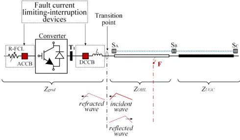
[image:7.612.50.295.371.514.2]should be immune against any practical fault current limiter, installed either on the AC or DC side. This will be better explained with the aid of Fig. 7.
Fig. 7. Explanation of travelling waves at a transition point.
A transition point is a point on a line where there is a change in surge impedance. When an electromagnetic wave passes through a transition point, a part of it is reflected, and a part continues to travel in the same direction [20], [21]. As indi-cated in Fig. 7, the initial wave is termed‘incident wave’, and the remaining two at the transition point are termed‘reflected wave’ and ‘refracted wave’. Any fault current limiting or interruption device is expected to increase the impedance (i.e.
Zgrid) and consequently affect the amplitude of reflected and refracted waves. However, no impact is expected on the time of arrival of the TW which is determined by the line impedance
ZOHLand distance to fault. Considering this and the fact that the sensors of the proposed scheme are installed on the line side of any potential fault limiting element (see Fig. 7) the performance of the scheme should not be compromised.
It should be noted that typical terminating inductors of
150 mH are already included in all the simulation results
presented in previous sections. In order to further validate the above reasoning, a fault occurring at 78.5 km on the UGC section of HTM-1 has been simulated with different fault current limiting and interruption technologies.
0 0.2 0.4 0.6 0.8 1 1.2 1.4 1.6 1.8 2
time [ms]
0 0.5 1
CWT Magnitude
L:100 mH L:150 mH L:300 mH DC-CB AC-CB R-FCL
Fig. 8. Normalized CWT magnitude for different fault current limiting technologies.
In particular inductive current limiters (with different in-ductance values), DC-CBs, AC-CBs, and AC resistive fault current limiters (R-FCLs) have been considered in the studies. DC-CBs represent a hybrid design as introduced in [11], R-FCL have been modelled according to [22], while the AC-CBs are represented by mechanical disconnectors.
The normalized CWT magnitudes (for wave detection) of these cases are depicted in Fig. 8, and the corresponding fault location errors have been reported as−0.0858%for all cases. The results in Fig. 8 have been generated by utilizing current measurements from sensors SA andSB as shown in Fig. 7. The results demonstrate that fault current limiters and breakers (either on DC or AC side) do not distort the time response of TWs at the specific point of measurement and hence the fault location accuracy is not affected.
G. Effect of Sampling Time and Small Increments of Fault Distance.
[image:7.612.315.554.385.470.2]UGC section of HTM-3. The results for PPFs at positions of 99 km to 101 km with steps of 100 meters have been generated. For this range of faults the error is shown in Fig. 9. The presented results were obtained by utilizing‘Haar’mother wavelet with a scaling factor α= 2.
99 99.2 99.4 99.6 99.8 100 100.2 100.4 100.6 100.8 101
Fault distance [km]
-0.3 -0.2 -0.1 0 0.1 0.2 0.3
[image:8.612.58.292.134.217.2]error [%]
Fig. 9. Fault location error with respect to small distance increment.
By moving fault position in short increments of 100 meters, an effect of randomly changing sampling instant is emulated. It has been established that the error can fluctuate between
−0.2489 % and 0.2489 %. This result has been achieved at very moderate sampling rate of 135kHz (used in all simula-tions presented in the paper). To reduce the sampling-time-related error, the sampling rate would have to be increased. Similar effect can be expected from all TW-based methods.
V. OPTICALSENSINGTECHNOLOGY
A. Transition Joint Pits
[image:8.612.314.563.324.462.2]Optical sensing technology for HVDC applications is a growing area of research and development. However, there are only a handful of field trials reported in open literature [23]–[25]. The purpose of such sensing schemes is to assist the implementation of protection, control, power quality and other power-system-related functions.
Fig. 10. Typical representation of a transition joint pit.
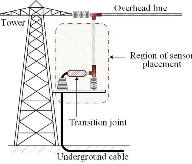
Optical sensing schemes (i.e. examples of optical current transformers) for HVDC applications are also reported in IEC-61689 [26] (Part 9: Standards for Digital Interface for Instrument Transformers). From the technical point of view, the connection between overhead lines and cables, is taking place at “transition joint pits (see Fig. 10), and the actual
conductor connection is established with ‘transition joints’ [27], [28]. Such pits are actual onshore installations with other protective, measuring and control components. Considering this, current optical sensors can be attached and installed around the transition joint and hence current measurements can be realized at transmission junctions.
B. Testing Methodology and Hardware Setup
In order to prove the principle of the proposed fault location scheme, the optical sensor system previously developed by the authors to enable distributed DC line monitoring was utilized in this study [11].
[image:8.612.75.268.476.641.2]The optical voltage sensor is formed by attaching an FBG to a piezoelectric transducer and measure strain generated as a result of a voltage applied across the transducer. The strain exerted on the FBG produces a corresponding shift in its peak wavelength which can be calibrated in terms of voltage. An analogous function can be achieved by utilizing a magnetostrictive transducer that responds to magnetic field generated around a conductor experiencing a fault current.
Fig. 11. Experimental setup schematic diagram.
Due to the working range of the utilized data acquisition card, the generated voltages were scaled to remain within a range of ±10 V. The voltage traces representing the DC line currents were then applied to the optical sensors while the corresponding measurement data obtained from the optical interrogation system was recorded on a PC for further pro-cessing by the fault location system algorithm developed in Matlab/SimulinkR.
was selected for demonstration as the most challenging case considering the number of segments and the length of lines.
Fig. 12. Laboratory experimental setup.
In the presented case, the HTM-3 section of the MTDC network (see Fig. 6) consisting of three segments and four optical sensors (SA, SB, SC, SD in Fig. 12) were considered. Pre-simulated fault currents at the corresponding four sensing locations along HTM-3 were used to provide replica voltage waveforms generated directly from a multi-function data ac-quisition card (installed on the National InstrumentsR PXI
unit). Prior to testing, the sensors were characterized and calibrated by applying a DC voltage across the piezoelectric transducers (in 1 V steps within the range of ±10 V). For all the corresponding voltages, the FBG peak wavelengths were recorded and the inverted function was used to calibrate wavelength shifts. The sampled data were stored on a PC for further analysis (e.g. signal processing, plotting, etc.)
The FBG peak wavelength shifts were monitored by a dedicated commercial FBG interrogation system (‘Sensors in-terrogator’ in Fig. 12) capable of acquiring the sensors spectra at 5 kHz. As such, the proposed fault location algorithm could only be demonstrated and practically validated at this relatively low sampling frequency. Nevertheless, the principle of operation and robustness of the proposed scheme has been fully validated (for all the three stages of the algorithm) even though with slightly lower accuracy of fault location. It should be noted, however, that the acquisition frequency limit of 5 kHz is strictly due to the FBG interrogator currently available for the experiments. Higher sampling rates can be achieved when alternative interrogators are employed, such as a solid state interrogator based on an Arrayed Waveguide Grating (AWG) previously developed by the authors [29], [30]. In such a case, the limiting factor for high speed operation would be the performance of the employed data acquisition and signal processing electronics, but scanning frequencies greater than 100 kHz can readily be achieved and the accuracy of the developed fault location prototype could be improved significantly.
C. Experimental Results
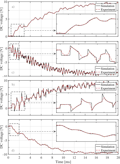
Time-domain waveforms recorded during the laboratory validation experiment are presented for fault scenarioF2only.
The summarized reposed to all the fault scenarios is presented in Table IX.
1) Measured response: The measured response from the sensors corresponding to fault scenario F2depicted in Fig. 11
is illustrated in Fig. 13. For the ease of comparison both simulation and experimental results are combined in the same figure.
0 2 4 6 8 10 12 14 16 18 20
Time [ms]
0 5 10
DC voltage [V]
Simulation Experiment
a)
0 2 4 6 8 10 12 14 16 18 20
Time [ms]
-10 -5 0
DC voltage [V] Simulation
Experiment
c)
0 2 4 6 8 10 12 14 16 18 20
Time [ms]
0 5 10
DC voltage [V]
Simulation Experiment
b)
0 2 4 6 8 10 12 14 16 18 20
Time [ms]
-10 -5 0
DC voltage [V] Simulation
Experiment
d)
Fig. 13. Simulated and experimental DC voltages corresponding to DC scaled fault currents for fault caseF2depicted in Fig. 11: a)S3−A, b)S3−B,S3−C,
b)S3−D.
The DC voltage traces shown above correspond to scaled-down replicas of the fault currents. It can be seen that all the dynamic features of the simulated currents are captured with some inevitable level of noise. However, it has been demonstrated in Section IV-E that the scheme is robust to noise originating from optical signal acquisition. It should be noted that due to the fault occurrence on the UGC there is a current reversal taking place between sensorsS3−BandS3−C. The shape of TWs in terms of frequency of reflections and waveform damping effect is a function of distance to fault and properties of the transmission media. The measurements
[image:9.612.313.552.109.436.2]2) Stage I - Faulted segment identification: For the exper-imental voltage traces illustrated in Fig. 13 the differential voltage Vdif f has been derived (corresponding to Idif f as explained in Section III-A) individually for every pair of adjacent sensors and is depicted in Fig. 14. The differential voltage calculated for the pair of sensors (i.e.S3−BandS3−C) adjacent to the faulted segment reaches much higher values compared to those related to healthy segments (i.e. S3−
A-S3−B and S3−C-S3−D). Therefore Stage I (faulted segment identification) of the proposed fault location algorithm is also verified experimentally.
0 2 4 6 8 10 12 14 16 18 20
Time [ms]
0 5 10 15
V diff
[V]
S3-A - S3-B
S 3-B - S3-C S
[image:10.612.51.298.204.296.2]3-C - S3-D
Fig. 14. Differential voltages calculated from experimental voltage traces for fault scenarioF2.
3) Stage II -Wave detection & fault location calculation:
The measurements from the sensors S3−B and S3−C have been utilized to perform CWT and calculate the arrival time of the TWs. The CWT for such measurements is depicted in Fig. 15. The time indices for fault location calculation correspond to t1(S3−B) = 0.760 ms and t1(S3−C) = 0.660
ms for the sensorsS3−B andS3−C respectively.
0 0.5 1 1.5
Time [ms]
0 0.5 1
CWT magnitude
S3-B
S 3-C
W TH
t1(S 3−B) t1(S
3−C)
Fig. 15. CWT calculated from experimental voltage traces from sensors S3−B andS3−C for fault scenarioF2.
4) Stage III - Fault location calculation: The summa-rized response of the three fault cases is presented in Ta-ble IX, where they are also compared with the simulation-based performance. As expected, the resulting accuracy of the experimentally-calculated fault location is slightly lower due to the reduced sampling rate (i.e. 5 kHz), determined by the available interrogation system. The sampling rate has an impact on the Wavelet Transform and the subsequent extraction of time difference ∆t(SU P−SDN) which is used in
equation (2) for fault distance calculation. This is also verified by observing the extracted time difference ∆t(SU P−SDN) for
each fault scenario. For fault scenariosF1,F2andF3the
sim-ulation based time difference is 0.16834 ms, 0.13183 ms and 0.10996 ms respectively. However, the time-difference values extracted from experiment have larger deviation compared to
those obtained from simulation, and hence larger errors. As demonstrated by the simulation results included in Section IV much better accuracy can be expected at higher sampling rates. The assumed rate of135 kHz at which the simulations were performed is technically achievable with commercially available upgraded equipment (this is currently unavailable in our laboratory facilities).
Regarding the faulted segment identification, it is evident from the reported sensors Sup −Sdn that it has been cor-rectly identified in all three cases, both for simulation and experimental-based analysis. Consequently, it can be con-cluded that the robustness of the proposed scheme is empiri-cally demonstrated.
TABLE IX
COMPARISON OFEXPERIMENTAL ANDSIMULATIONSRESULTS
Faults F1 F2 F3
Error [%]
Sim. 0.4583 -0.2489 0.4806 Exp. -1.3254 -1.3415 1.0652
|∆t(SU P−SDN)| [µs]
Sim. 0.17037 0.12592 0.11110 Exp. 0.16249 0.10000 0.11250 Reported sensors
SU P−SDN
Sim. S3−A, S3−B S3−B, S3−C S3−C, S3−D
Exp. S3−A, S3−B S3−B, S3−C S3−C, S3−D
VI. CONCLUSIONS
A new fault location scheme suitable for hybrid networks with segments of overhead lines and underground cables has been proposed. The scheme relies on the measurements obtained from a network of distributed current optical sensors, and it uses travelling wave principle to estimate the fault position.
The proposed algorithm has been found to successfully identify the faulted segment of the line in all cases regardless the position of the fault (i.e. OHL or UGC) or the number of series-connected segments, which verify and demonstrate its robustness. The scheme has also be found to consistently maintaining high accuracy of the fault location estimation across a wide range of fault scenarios including both pole-to-pole and pole-to-ground faults with resistances up to 500
Ω. Assuming a sampling rate of 135 kHz, and using the mother wavelet ‘coif2’ with scaling factor α = 4, the maximum fault location error has been found to be 0.1677% while the average error is0.0784%. Additionally the proposed scheme has been found to be robust against noisy inputs for a wide range of mother wavelets and scaling factors. Studies have included the impact of fault current limiting and interruption devices installed both on AC and DC side and the accuracy of the proposed scheme was found to be immune when such devices are utilized. A hardware prototype based on FBG optical sensors has been employed to conduct a series of laboratory tests which confirm the practical feasibility of the proposed scheme, while demonstrating the robustness for faulted segment identification. A few considerations regarding the installation of the sensors at the transition points of transmission lines and underground cables have also been reported.
REFERENCES
[image:10.612.316.561.246.327.2]failure,”IEEE Transactions on Power Delivery, vol. 31, no. 2, pp. 789– 797, April 2016.
[2] D. Tzelepis, A. O. Rousis, A. Dysko, C. Booth, and G. Strbac, “A new fault-ride-through strategy for MTDC networks incorporating wind farms and modular multi-level converters,”Electrical Power and Energy Systems, vol. 92, pp. 104–113, November 2017.
[3] W. Leterme, P. Tielens, S. D. Boeck, and D. V. Hertem, “Overview of grounding and configuration options for meshed HVDC grids,”IEEE Transactions on Power Delivery, vol. 29, no. 6, pp. 2467–2475, Dec 2014.
[4] A. Raza, X. Dianguo, L. Yuchao, S. Xunwen, B. W. Williams, and C. Cecati, “Coordinated operation and control of VSC based multiter-minal high voltage DC transmission systems,” IEEE Transactions on Sustainable Energy, vol. 7, no. 1, pp. 364–373, Jan 2016.
[5] O. Nanayakkara, A. Rajapakse, and R. Wachal, “Location of DC line faults in conventional HVDC systems with segments of cables and overhead lines using terminal measurements,” IEEE Transactions on Power Delivery, vol. 27, no. 1, pp. 279–288, Jan 2012.
[6] M. Farshad and J. Sadeh, “A novel fault-location method for HVDC transmission lines based on similarity measure of voltage signals,”IEEE Transactions on Power Delivery, vol. 28, no. 4, pp. 2483–2490, Oct 2013.
[7] O. Nanayakkara, A. Rajapakse, and R. Wachal, “Traveling-wave-based line fault location in star-connected multiterminal HVDC systems,”IEEE Transactions on Power Delivery, vol. 27, no. 4, pp. 2286–2294, Oct 2012.
[8] L. Yuansheng, W. Gang, and L. Haifeng, “Time-domain fault-location method on HVDC transmission lines under unsynchronized two-end measurement and uncertain line parameters,” IEEE Transactions on Power Delivery, vol. 30, no. 3, pp. 1031–1038, June 2015.
[9] S. Azizi, M. Sanaye-Pasand, M. Abedini, and A. Hasani, “A traveling-wave-based methodology for wide-area fault location in multiterminal DC systems,”IEEE Transactions on Power Delivery, vol. 29, no. 6, pp. 2552–2560, Dec 2014.
[10] H. Livani and C. Y. Evrenosoglu, “A single-ended fault location method for segmented HVDC transmission line,”Electric Power Systems Re-search, vol. 107, pp. 190–198, 2014.
[11] D. Tzelepis, A. Dyko, G. Fusiek, J. Nelson, P. Niewczas, D. Vozikis, P. Orr, N. Gordon, and C. D. Booth, “Single-ended differential protection in mtdc networks using optical sensors,”IEEE Transactions on Power Delivery, vol. 32, no. 3, pp. 1605–1615, June 2017.
[12] J. D. Shin and J. Park, “Plastic optical fiber refractive index sensor employing an in-line submillimeter hole,”IEEE Photonics Technology Letters, vol. 25, no. 19, pp. 1882–1884, Oct 2013.
[13] EU, “Twenties project - final report,” Tech. Rep., Oct 2013.
[14] T. C. Peng, D. Tzelepis, A. Dysko, and I. Glesk, “Assessment of fault location techniques in voltage source converter based HVDC systems,” inIEEE Texas Power and Energy Conference, Feb 2017, pp. 1–6. [15] K. Nanayakkara, A. D. Rajapakse, and R. Wachal, “Fault location in
ex-tra long HVDC ex-transmission lines using continuous wavelet ex-transform,” inInternational Conference on Power Systems Transients, April 2011. [16] X. Dong, J. Wang, S. Shi, B. Wang, B. Dominik, and M. Redefern,
“Traveling wave based single-phase-to-ground protection method for power distribution system,”CSEE Journal of Power and Energy Systems, vol. 1, no. 2, pp. 75–82, June 2015.
[17] Q. Yang, S. L. Blond, F. Liang, W. Yuan, M. Zhang, and J. Li, “Design and application of superconducting fault current limiter in a multitermi-nal HVDC system,”IEEE Transactions on Applied Superconductivity, vol. 27, no. 4, pp. 1–5, June 2017.
[18] L. Zhang, J. Shi, Z. Wang, Y. Tang, Z. Yang, L. Ren, S. Yan, and Y. Liao, “Application of a novel superconducting fault current limiter in a VSC-HVDC system,”IEEE Transactions on Applied Superconductivity, vol. 27, no. 4, pp. 1–6, June 2017.
[19] Z. Shuai, P. Yao, Z. J. Shen, C. Tu, F. Jiang, and Y. Cheng, “Design considerations of a fault current limiting dynamic voltage restorer (FCL-DVR),”IEEE Transactions on Smart Grid, vol. 6, no. 1, pp. 14–25, Jan 2015.
[20] F. Lopes, K. Dantas, K. Silva, and F. B. Costa, “Accurate two-terminal transmission line fault location using traveling waves,”IEEE Transac-tions on Power Delivery, vol. PP, no. 99, pp. 1–1, 2017.
[21] L. Tang, X. Dong, S. Luo, S. Shi, and B. Wang, “A new differential protection of transmission line based on equivalent travelling wave,” IEEE Transactions on Power Delivery, vol. 32, no. 3, pp. 1359–1369, June 2017.
[22] A. R. Fereidouni, B. Vahidi, and T. H. Mehr, “The impact of solid state fault current limiter on power network with wind-turbine power
generation,”IEEE Transactions on Smart Grid, vol. 4, no. 2, pp. 1188– 1196, June 2013.
[23] K. Bohnert, H. Brandle, M. G. Brunzel, P. Gabus, and P. Guggenbach, “Highly accurate fiber-optic DC current sensor for the electrowinning industry,”IEEE Transactions on Industry Applications, vol. 43, no. 1, pp. 180–187, Jan 2007.
[24] M. Takahashi, K. Sasaki, Y. Hirata, T. Murao, H. Takeda, Y. Nakamura, T. Ohtsuka, T. Sakai, and N. Nosaka, “Field test of DC optical current transformer for HVDC link,” inIEEE PES General Meeting, July 2010, pp. 1–6.
[25] Y. Hirata, K. Sasaki, M. Takahashi, H. Aizawa, H. Takeda, Y. Ishida, N. Nosaka, and T. Sakai, “Application of an optical current transformer for cable head station of hokkaido-honshu HVDC link,” inPES T D 2012, May 2012, pp. 1–6.
[26] “IEC 61869-9: ED 1.0 instrument transformers - part 9: Digital interface for instrument transformers,”BSI, 2013.
[27] T. Igi, Y. Murata, K. Abe, M. Sakamaki, S. Kashiyama, and S. Katakai, “Advanced HVDC XLPE cable and accessories,” in 9th IET Interna-tional Conference on Advances in Power System Control, Operation and Management, Nov 2012, pp. 1–6.
[28] G. Mazzanti and M. Marzinotto, Extruded Cables for High Voltage Direct Current Transmission. IEEE PRESS - Wiley, 2013.
[29] G. Fusiek, P. Niewczas, and J. R. McDonald, “Concept level evaluation of the optical voltage and current sensors and an arrayed waveguide grat-ing for aero-electrical systems’ applications,” inIEEE Instrumentation Measurement Technology Conference, May 2007, pp. 1–5.
[30] G. Fusiek, P. Niewczas, and J. McDonald, “Feasibility study of the application of optical voltage and current sensors and an arrayed waveguide grating for aero-electrical systems,”Sensors and Actuators A: Physical, vol. 147, no. 1, pp. 177 – 182, 2008.
Dimitrios Tzelepis (S’13 - M’17) received the B.Eng. in Electrical Engineering and the M.Sc in Wind Energy Systems from Technological Educa-tion InstituEduca-tion of Athens (2013) and University of Strathclyde (2014) respectively. He is currently pursuing his Ph.D. at the department of Electronic and Electrical Engineering, University of Strath-clyde, Glasgow, U.K. His main research interests include power systems protection; implementation of intelligent algorithms for protection, fault location and control applications; and HVDC transmission.
Grzegorz Fusiek(M’11) received the M.Sc. degree in Electrical Engineering from the Lublin University of Technology, Poland, in 2000 and the Ph.D. degree in the area of interrogation systems for spectrally encoded sensors from the University of Strathclyde, Glasgow, UK, in 2007. He is a Research Fellow within the Institute for Energy and Environment in the Electronic and Electrical Engineering De-partment, University of Strathclyde. His interests concentrate on the optical sensing techniques for power industry and energy systems applications.
Pawel Niewczas (M’05) is a Reader in the De-partment of Electronic and Electrical Engineering at the University of Strathclyde. He is leading the Advanced Sensors Team within the Institute for En-ergy and Environment in the same department. His main research interests centre on the advancement of photonic sensing methods and systems integration in applications that lie predominantly in power and energy sectors.
Campbell Booth received the B.Eng. and Ph.D. degrees in electrical and electronic engineering from the University of Strathclyde, Glasgow, UK in 1991 and 1996, respectively. He is currently a Profes-sor and Head of Department for Electronic and Electrical Engineering, University of Strathclyde. His research interests include power system pro-tection; plant condition monitoring and intelligent asset management; applications of intelligent system techniques to power system monitoring, protection, and control; knowledge management; and decision support systems.
![Fig. 5). The thresholdT Harrival time has been set to 0.25. As also discussed in [7] the used for establishing the wavevalue of the threshold is subject to the assumed safety margins,](https://thumb-us.123doks.com/thumbv2/123dok_us/1495785.102270/5.612.316.559.82.504/thresholdt-harrival-discussed-establishing-wavevalue-threshold-subject-assumed.webp)