City, University of London Institutional Repository
Citation:
Ciulla, F., Perra, N., Baronchelli, A. and Vespignani, A. (2014). Damage
detection via shortest-path network sampling. Physical Review E (PRE), 89(5), 052816. doi:
10.1103/PhysRevE.89.052816
This is the accepted version of the paper.
This version of the publication may differ from the final published
version.
Permanent repository link:
http://openaccess.city.ac.uk/4779/
Link to published version:
http://dx.doi.org/10.1103/PhysRevE.89.052816
Copyright and reuse: City Research Online aims to make research
outputs of City, University of London available to a wider audience.
Copyright and Moral Rights remain with the author(s) and/or copyright
holders. URLs from City Research Online may be freely distributed and
linked to.
Fabio Ciulla,1 Nicola Perra,1 Andrea Baronchelli,2 and Alessandro Vespignani1, 3
1Laboratory for the Modeling of Biological and Socio-technical Systems,
Northeastern University, Boston MA 02115 USA
2
Department of Mathematics, City University London, Northampton Square, London EC1V 0HB, UK
3Institute for Scientific Interchange (ISI), Torino, Italy
(Dated: January 30, 2014)
Large networked systems are constantly exposed to local damages and failures that can alter their functionality. The knowledge of the structure of these systems is however often derived through sampling strategies whose effectiveness at damage detection has not been thoroughly investigated so far. Here we study the performance of shortest path sampling for damage detection in large scale networks. We define appropriate metrics to characterize the sampling process before and after the damage, providing statistical estimates for the status of nodes (damaged, not-damaged). The proposed methodology is flexible and allows tuning the trade-off between the accuracy of the damage detection and the number of probes used to sample the network. We test and measure the efficiency of our approach considering both synthetic and real networks data. Remarkably, in all the systems studied the number of correctly identified damaged nodes exceeds the number false positives allowing to uncover precisely the damage.
PACS numbers: 89.75.-k,89.75.Hc,89.20.Hh
Real world networks are often the result of a self-organized evolution without central control [1–3]. The physical Internet and the World Wide Web are two pro-totypical examples where the interplay of local and non-local evolution mechanisms defines the global structure of the network. In absence of defined blueprints, the only way to characterize the global structure of self-organizing systems is by devising sampling experiments, liketraceroute probing for the physical Internet [4–9] and web crawlers for the WWW [10–12], that try to infer the properties and connectivity patterns of these struc-tures [13–19]. However, sampling processes are limited by time and physical constraints, and in general guaran-tee access only to a part of the network. In this context, the detection of network damage is a difficult task. The lack of information on the exact structure of the sys-tem makes it extremely difficult to identify what damage has been actually suffered and discriminate damaged el-ements from those that have been simply not yet probed by the sampling process.
Here we study numerically the effectiveness of shortest path sampling strategies for damage detection in large-scale networks. Shortest path sampling strategies are ac-tually used in Internet probing [1, 20–24] including fail-ure detection, via traceroute like tools and end-to end measurements. We consider different attack strategies, namely random or connectivity based and introduce a global measure,M, that allows to quickly identify dam-ages that induce large variations in the routing patterns of networks. We then propose a statistical method able to classify nodes as damaged or functioning in the case of partial network sampling. In our analysis, we first sam-ple a given network structure via shortest path probes [1, 20–24] obtaining a partial representation of its nodes and connectivity patterns. Then we damage the
net-work by removing nodes according to different strategies and sample again the damaged network supposing not to know the location and magnitude of the damage. Dur-ing this samplDur-ing, we constantly monitor whether the probability not to have seen a node exceeds the expected value calculated on the basis of the sampling of the un-damaged graph. We define a statistical criterion to asses which nodes of the network can be considered damaged, and we test the performance of the method by looking at the number of true and false positives it identifies.
We perform numerical experiments on synthetic net-works, either heterogeneous, generated with the un-correlated configurational model (UCM) [25], or ho-mogeneous, obtained through the Erd¨os-R`eny model (ER) [26]. Remarkably, the magnitude and location of the damage can be detected with fairly good confidence. The accuracy improves for nodes that play a central role in network’s connectivity. Namely, the detection of dam-aged hubs is more reliable than the one of peripheral nodes. As a practical application, we consider the dam-age detection on the physical Internet at the level of Au-tonomous System (AS). We use the AS topology pro-vided by the Dimes project [14]. In this case, to sim-ulate realistic damages, we remove nodes according to their geographical position. In doing so we simulate crit-ical events such as large-scale power outages, deliberate servers switch offs [27] or other major localized catas-trophic events [28]. Interestingly, also in this case our methodology allows to statistically identify the extent and location of the damage with reasonable accuracy.
The paper is organized as follows: in the section I we present the sampling method used. In section II we introduce a measure that provides a general estimation of the damage extension in sampled networks. In section III we provide a method to infer if a single node is
2
damaged or not using a p-value test. In section IV we validate this method by applying it to the physical Internet network. Finally in section V we present our conclusions and final remarks.
SHORTEST PATH SAMPLING OF UNDAMAGED NETWORKS
The sampling of networks via shortest paths consists in sending probes from a set of nodes that have been de-fined as sources toward another set of nodes chosen to be targets. Each probe travels through the network follow-ing a shortest path and records each node and link visited returning a path. This is, to a first approximation, what is executed by Internet mapping projects that use the traceroute tool [8] as probing method. This methodology infers paths by transmitting a sequence of limited-time-to-live TCP/IP packets from a source node to a specified target on the Internet. The nodes visited along the way send their IP addresses as a response and create the path. The union of all the paths returned by the probes creates the sampled picture of the network. However, mapping the real physical Internet is complicated and existing ap-proaches have major limitations [4]. For example, visited nodes can fail to provide their IP address, and wrong or outdated forwarding routes registries can result in not optimal forwarding route indications. Our study is in-spired by the traceroute tool although we assume that our probes follow shortest paths in the network neglect-ing the real world limitations aforementioned.
Here we focus on undirected and unweighted networks constituted of N nodes and M edges G(N, M). We fix a set of sourcesS= (s1, s2, . . . , sNS) and a set of target
T= (t1, t2, . . . , tNT) among the N nodes, beingNS and
NT the total number of sources and targets respectively.
For each pair of nodes, taken in the two sets, a shortest path probe is sent. After all of the NS×NT probes are
executed, all the resulting paths are merged in a sampled network that we denote as G∗(N∗, M∗). Here and in the rest of the paper the star symbol indicates sampled quantities, soN∗ is the number of discovered nodes and
M∗ the number of discovered links via to the shortest path sampling.
In general, for each source-destination pair we can have two or more equivalent shortest paths. More precisely, there could be different strategies to numerically simulate the shortest path probing:
• Unique shortest path (USP). The shortest path be-tween a node i and a targetT is always the same independently of the source S. Each shortest path is selected initially and they will never change.
[image:3.612.337.544.51.148.2]• Random shortest path (RSP). Each shortest path is selected every time randomly among the equivalent
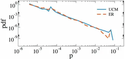
FIG. 1: Probability distribution function (pdf) of node visit probability for undamaged UCM (blue solid line) and ER (or-ange dashed line) networks. The two peaks that deviate from the overall heavy-tailed behavior occurs at pi = 1/NS and pi= 1/NT, and represent the visit probability of sources and
target respectively. The curves are the average over 100 in-dependent simulations.
ones.
• All shortest path (ASP). All possible, equivalent, shortest path between shortest path are discovered.
In the following we will use the RSP probing strategy [20, 29–31]. Both sources and targets are chosen randomly among all the nodes. Inspired by real Internet probing we investigate scenarios in which the order of magnitude of sources isNS =O(10), while the order of magnitude
of density of targets,ρT, isO(10−1). Along with the raw
number of discovered nodes, we also keep track of the visit probabilitypi for each visited nodei, defined as the
ratio between the number of shortest path probes passed through the nodeiand the total number of probes sent
NS×NT:
pi=
NS×NT P
j=1
δi,j
NSNT
, (1)
whereδi,j is equal to 1 if the nodeiis seen by the probe
j. In the limit in which bothNS and NT approach N,
the probabilitypbecome the betweenness [20]. Instead, in more realistic cases in which the number of sources and targets is small the nodes visit probability is just an approximation of this quantity [20]. Considering this limit, we show the distribution ofpin Figure 1 in both UCM and ER networks with 105 nodes. The number of
sources is 15 and the target density is 0.2. The curves show a power law behavior except for the presence of two peaks, representing the visit probability of sources and targets. The peak for large values ofpiis the consequence
of the visit of sources, and appears in correspondence of
pi =psource = 1/NS, ∀i∈S. The other peak is due to
DAMAGE DETECTION
In order to introduce damage in the network, we con-sider that ND nodes are not functional, i.e. a fraction
ρD = ND/N, of nodes and all their links are removed
from the network G. We define the damaged network
GD(ND, MD) where the subscript D denotes damage.
Damaged nodes are selected either randomly or accord-ing to a degree based strategy in which nodes are re-moved according to their position in the degree ranking (hubs first or leafs first). Although probes target nodes can be damaged, we assume that no sources are dam-aged. In these settings we aim at inferring the damage using shortest path sampling by looking at the number of nodes discovered before and after the damage occurs. Shortest path probes are sent between each pair of source-target nodes. The sampled network after the dam-age G∗
D differs in general from the sampled view G∗ of
the original undamaged network because of the changed topology due to the missing nodes. To quantify the dam-age we introduce the quantity
M = 1−N
∗
D
N∗ (2)
whereN∗andND∗ are the number of discovered nodes in the undamaged and damaged network respectively. If no damage occurs, the number of nodes discovered inGD is
similar to the one discovered inG so thatN∗'ND∗ and
M '0 [38]. If less nodes are seen in GD than inG then
M > 0, with M = 1 representing the extreme case in
which no nodes are discovered in the damaged network. Interestingly, the quantity M can assume also negative values. Indeed, it is possible to see more nodes in GD
respect to G. Although this case may sound counterin-tuitive at first, a closer look to the effect in the topology induced by removing nodes, clearly explain its meaning. Indeed, by removing some central nodes in the network (in the next section we discuss this point in details) the length of the shortest paths might increase on average as well as the number of discovered nodes.
Numerical simulations
We measure the quantityM in damaged homogenous and uncorrelated heterogenous networks [1–3, 32], gen-erated through the ER and the UCM algorithm, respec-tively. The network size is fixed at N = 105 nodes, and
the number of sources and target density are NS = 15,
andρT = 0.2, respectively. The average degree is ¯k= 8
[image:4.612.336.542.48.255.2]for both the topologies. The exponent γ for UCM is 2.5. As mentioned above, sources and targets are ran-domly selected. We consider different damage strategies in which the removed nodes are selected at random or considering their degree. We further divide the latter
FIG. 2: The behavior of M is shown for three different damage strategies: random (red squares), small degree nodes first (green diamonds) hubs first (blue circles). (A) UCM scale-free graph. Inset: the behavior ofM when high degree nodes are removed first is compared to the quantityhliρavas
a function ofρD. (B) ER random graph. For UCM network
the minimum indicates the enhanced discovery given by the lack of hubs. Each plot is the median among 10 independent assignment of sources and targets.
strategy considering two cases in which nodes are re-moved in increasing (hubs first) or decreasing order of degree.
Figure 2 shows M as a function of ρD for the three
different attack mechanisms, for the two different types of network. The top panel presents data for UCM net-work. The random nodes removal strategy gives the same qualitative behavior as the one in which the small degree nodes are attacked first. This is not surprising, since the probability that a randomly selected node has small degree is extremely high due to the power-law degree dis-tribution of the network. The two strategies select, on average, the same category of nodes. A big difference can be noted when nodes are attacked in decreasing order of degree (high degree nodes, hubs, are attacked first). For small values ofρD the value ofM assumes negative
val-ues, meaning that more nodes are discovered in the dam-aged network than in the undamdam-aged one. Indeed, hubs act as shortcuts for network connectivity. Their failure causes the rerouting of probes toward lower degree nodes and the consequent growth of the average length of the shortest paths hli. As ρD increases, this trend is
con-trasted by the progressive fragmentation of the network in many disconnected components.
In order to estimate how much the network has been fragmented by the damaging process we define the quan-tity ρav as the average of the ratio between the nodes
4
the total number of nodesN of the undamaged network. After a certain amount of nodes are removed, the graph undergoes disconnection and more than one component appears. At this point a shortest path probe can reach only the nodes belonging to the component where the source is located. Components with no sources will be no longer accessible. ρav is a decreasing function ofρD
assuming the value 1 when there is no damage, whereas it becomes ρav =NS/N in the limit ofρD '1, when only
the sources survive and each of them constitutes one com-ponent. Neitherhliorρav alone explains the presence of
the minimum of the quantityM in the plots. Instead the product of the twohliρav does: it represents the average
number of nodes discovered by each shortest path probe rescaled by the number of nodes effectively available to be discovered. The relation of this quantity with the minimum forM is shown in the inset of Figure 2A. The argument above is confirmed by the behavior ofM in ER graphs. Here, removing the nodes with higher degree has a much smaller impact on the topology, and consequently there is no increase in the amount of nodes discovered in the damaged graphGD with respect to the original one G. The plot of M for hubs removal in the ER network does not show a minimum and substantially the damage detection works similarly for all damage strategies.
SINGLE NODE DAMAGE DETECTION
While the measure M quantifies the damage at the global level, it does not provide any information about specific nodes of the network. In this section we address the damage of individual nodes by assuming that the information gathered during the exploration of the un-damaged network constitutes the null hypothesis of our measure, namely that no one of the nodes is damaged. We start by monitoring the networkGassuming that it is not damaged. Every time we send a shortest path probe we obtain a better approximation of the sampled network
G∗ with increasing number of discovered nodesN∗. At the same time we collect information about how many times a probe passes through a nodei resulting on visit probabilitypidefined in Eq. 1. The network is then
dam-aged according to one of the strategies discussed above, and sampled via shortest path probes. By definition, any node that is discovered during the sampling is not dam-aged. However, the situation is less clear for nodes that have not been discovered. Indeed, the reason why a node is not seen can be either that it is actually damaged or that the sampling has missed it because the damage has altered the shortest path routing.
In order to infer the state of undiscovered nodes we use a p-value test [33] applied to the visit probabilitypi.
More precisely, we calculate the probability (1−pi)τ of
[image:5.612.335.543.50.221.2]not seeing the node iafter a number τ of shortest path probes. τ can assume any integer value from 1 to NS×
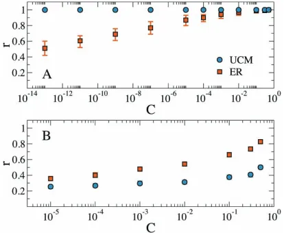
FIG. 3: Precisionαas a function ofCfor (A) hubs removal with fraction of removed nodesρD = 0.001 and (B) random
nodes removal with fraction of removed nodesρD= 0.01. The
black dashed line indicateα= 0.9. Dots represent the average over 100 independent simulations and error bars illustrate the 95% confidence interval.
NT. The p-value test consist in imposing the equality
between this quantity and an arbitrary confidence level
C:
C= (1−pi)τi (3)
Note that after imposing the equality, τi has the index
ias forpi. This is because τi is different for each node.
By taking the logarithm on both side of the equation we obtain:
τi=
lnC
ln(1−pi)
(4)
If the node i has not been seen at least once before τi
probes have been sent then we can state thatiis damaged with statistical confidenceC. Here we are assuming that the visit probability of nodes does not change after the damage. This holds when the damage is a relatively small perturbation and does not change the connectivity of the network or its dynamical properties [3, 34, 35]. After the pi values have been determined for all the nodes,
the value of C tunes the number of probes to be sent before declaring a node damaged. IfC is selected to be large, nodes will be considered as damaged much earlier but with a small statistical confidence, leading to a large number of false positive (F P) detections. Conversely, if
C is set to be small, more probes are needed to state if a node is damaged or not. The accuracy improves and the final response will eventually return only actually damaged nodes, the true positive damaged nodes (T P). On the other hand the number of probes needed to reach this level of statistical confidence will be much higher resulting in a longer sampling process.
FIG. 4: Probability distribution function (pdf) of nodes visit probability in the undamaged UCM (A) and ER (B) networks restricted to nodes that will be later damaged with two dif-ferent strategies.Curves are the average over 100 independent simulations.
a poor but fast sampling that produces high number of
F Ps and an accurate but slow sampling that generates moreT Ps. We evaluate the performances of the damage detection strategy measuring its precision and recall. In particular, the precision,α, is defined as
α= T P
T P +F P. (5)
The recall,r, is instead
r= T P
T P +F N, (6)
where F N indicates the number of false negatives, i.e. nodes damaged but not detected. In a given network precision and recall are functions of the parameter C. In Figure 3 we plot α for different values of C in both UCM and ER networks. In the top panel we remove top degree nodes and set ρD = 10−3. As expected α
increases as C decreases. Interestingly, in the case of UCM topologies the increase is slower. Indeed, we can notice that αreaches an arbitrary level of 90% (dashed line) forC= 10−10while in the case of ER networks the
same level is reached for C = 10−5. The extremely low values of C, above all in the case of the UCM network, is justified by the presence of the logarithm function at the numerator of Eq. 4. Considering the big absolute value of the denominator for big pi, very low values of C are
required to have values ofτi that possibly ranges from 0
to NS ×NT. The quite different value of C in the two
networks for top degree nodes removal can be explained considering the distribution of pi of the damaged nodes
[image:6.612.73.280.49.218.2]in case of hubs removal as shown in Figure 4. In the UCM network top degree nodes have much higher visit probability respect to the rest of the nodes. In the ER network, instead, the role of high degree nodes is not
FIG. 5: Recall r as a function of C for (A) hubs removal with fraction of removed nodesρD = 0.001 and (B) random
nodes removal with fraction of removed nodes ρD = 0.01.
Dots represent the average over 100 independent simulations and error bars illustrate the 95% confidence interval.
so determinant and the visit probability of high degree nodes is almost indistinguishable from the one of random nodes. For the same value of C in Eq. 4 the difference in pbetween UCM and ER translates in smaller values ofτifor the UCM network. This leads to higher number
of FPs and hence smaller precision. In Figure 3B we show the same curve for the random damaging strategy setting ρD = 10−2. In this case the behavior of α in
the two topologies is very similar. Such behavior is due to the p distributions that in both networks span the entire range of possible visit probabilities irrespective of the topology reproducing the same behavior shown in Figure 1.
In Figure 5 we study the recall r as a function of C. In this case we can see thatrreaches 1 for all the values ofC investigated when damaging hubs in an UCM net-work. All damaged nodes are detected during the sam-pling. This is consequence of the very large visit proba-bilities for high degree nodes in the UCM network. In-deed, largepis combined withCvia Eq. 4, produce small
values ofτi, allowing all removed nodes to be promptly
declared damaged. The downside of this effect is the lack of precision for large values ofC (see Figure 3). In the ER network, instead, the presence of low visit probabil-ity nodes among the ones in the top degree ranks makes their discovery more lengthy. Indeed, in this case larger values ofC are required to produce τis small enough to
allow the algorithm to declare the nodes damaged. It is crucial to stress thatτmax =NS×NT. Any node that
for a given C is characterized by τi > τmax will not be
[image:6.612.336.543.51.221.2]6
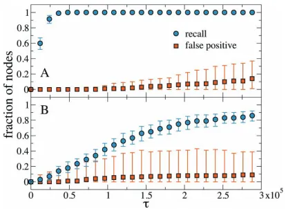
FIG. 6: Recallr(blu circles) and normalized number of false positivef p(orange squares) for high degree nodes removal as a function of number of probes in UCM (A) and ER (B) networks. The fraction of removed nodes isρD= 0.001. The
values of confidence level C are 10−10 and 10−5 for UCM and ER networks respectively. Points are the median among 100 realization with independent choice of sources and target. Error bars illustrate the 95% confidence interval.
networks as consequence of the similar visit probability distributions.
Numerical simulations in synthetic networks
We apply the statistical criterion developed in the pre-vious section to the two types of synthetic networks, UCM and ER, with 105nodes and two damaging strate-gies, high degree and random nodes removal. We send shortest path probes from 15 sources to a number of tar-gets equal to a fractionρT = 0.2 of total nodes. In order
to compare the results of this part of the study for differ-ent topologies and damage strategies we arbitrarily fixed the C value to the one correspondent to a precision of
α= 0.9 in each system.
Let us first consider UCM networks subject to the re-moval of the top hundred nodes ranked according to the degree (ρD= 10−3). In Figure 6 we plot the recall,r, and
the normalized number of FPs, f p = F P/(T P +F N) as a function of τ. Interestingly, the recall reaches 1 quickly. The absence of the hubs is promptly detected by the method. In Figure 7 we show the behavior of the same quantities in the case of random removal of nodes considering ρD = 10−2. In this case the recall increase
slowly whilef premains constant after an initial increase. An interesting feature of thercurve is the presence of a jump. This jump is the consequence of the peak in the distribution ofpi that is mapped intoτivia Eq. 4. It
oc-curs at the value ofτ corresponding toptargets= 1/NT
[image:7.612.73.280.49.200.2]and is caused by the enhanced visit probability of tar-get nodes. Since tartar-gets are assigned randomly, in UCM networks they are most probably small degree nodes that are visited just if they are set to be targets. This imply
FIG. 7: Recall r (blu circles) and normalized number of false positivef p(orange squares) for random nodes removal as a function of number of probes in UCM (A) and ER (B) networks. The fraction of removed nodes isρD = 0.01. The
value of confidence levelCis 10−3for both the UCM and ER network. Points are the median among 100 realization with independent choice of sources and target. Error bars illustrate the 95% confidence interval.
that a specific number of probes equal to
τtargets=
lnC
ln(1−ptargets)
= lnC
ln(1−1/NT)
(7)
is necessary to be able calling targets as damaged or not. Since targets are 20% of the nodes, onceτtargets is
reached a conspicuous amount of nodes is characterized by the p-value test. It is worth noting that only the num-ber of T Ps increases in correspondence with the jump, andf pdo not exhibit any discontinuity. This means that we have a better view of the damage without affecting the accuracy.
Let us now consider ER networks subject to removal of nodes in decreasing order of degree. In Figure 6B we plotrandf pas a function ofτ. As for the case of UCM network, the recall increases, even if slower, and reaches the maximum values at 0.9. Similar behavior for both the topologies is observed in the case of random removal of nodes (see Figure 7).
NUMERICAL DAMAGE DETECTION IN GEOLOCALIZED NETWORKS
In this section we consider a sample of the real In-ternet topology network at the level of ASs where each node is an autonomous system of known geographical lo-cation [13, 21, 36], and links represent the physical con-nections among them. Topologies are available for down-loads in the DIMES project webpage [14]. We focus on the largest connected component of ASs that is made by 32852 nodes.
[image:7.612.336.544.49.201.2]at-FIG. 8: Europe map showing the detected Italian damaged nodes in the real AS network. Each circle represent one AS and its size is proportional to the degree. Green circles are the working nodes, blue ones are the TPs while orange ones are the FPs. Nodes located at sea are effect of finite accuracy of geographical coordinates provided.
tacked, and all nodes inside a radiusξ with epicenterE
are attacked. Both of these strategies are geography-based but they provide different scenarios. The first represents a deliberate shut down, for instance as al-legedly happened in several countries during the Arab spring [27]. The second one is referred to localized event such as blackouts, earthquakes, or others catastrophic events [28]. Also in this case we fix the number of sources
NS = 15 and the density of targetsρT = 0.2. According
to one of the two geographic based strategies we remove
NDnodes from the original AS network. The main
differ-ence between this case and those discussed in the previous sections is that the networks here have geographical at-tributes. The measure of damage detection should then be able to return not only the entity of the damage as a whole, but also tell us where the damage is localized.
We use the same method already discussed for syn-thetic networks. As an example of entire country switch off we decided to damage all the AS nodes in Italy. This translates in removingND= 1246 nodes, equal to a
frac-tionρD= 0.038 of total nodes. Figure 8 shows the
out-come of our analysis. We want to stress that the algo-rithm does not have any a priori information about the location of the damage. Despite that, the method clearly returns Italy as affected country. Few other nodes are wrongly classified as damaged. The reason for the pres-ence of FPs can be just statistical fluctuations or, more interesting, that some FP nodes turn out to be strongly linked to the Italian TPs, so that the deletion of the lat-ter prevents them to be visited. For the second type of geographical damage we decide to switch off all the ASs within a radius of 50 km around the city of Boston, MA, in the USA. This corresponds to ND = 176 and
ρD = 0.0054. Also in this case the method is able to
detect correct location of the damage as shown in
Fig-FIG. 9: Map of part of the United States east coast showing the outcome after damaging nodes around the city of Boston within a radius of 50 km in the real AS network. Each circle represent one AS and its size is proportional to the degree. Green circles are the working nodes, blue ones are the TPs while orange ones are the FPs.
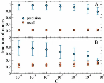
ure 9. In both cases of geographical damaging the recall is almost constant and close to the value 0.2 as shown in Figure 10. Indeed, the algorithm is detecting almost only the fraction of damaged nodes that are also target. Because of the homogeneous distribution of target nodes, this fraction corresponds toρT = 0.2. The choice for the
statistical confidence affects more the measures related to local damaging (Figure 10B). Here, for big values of
C the precision drops while the recall slightly increases. This means that a less strict choice ofC allows the dis-covery of more nodes. However the FPs grow more than the TPs. So a little gain in recall is contrasted by big loss in precision. As for the artificial networks, in the case of entire country damaging we chooseC to achieve a pre-cision of 0.9 (C = 10−2). In the case of local damaging
there is no value ofC that allow to reach such a preci-sion. For this reason and considering the diverse nature of the two strategies we fix the arbitrary value toα= 0.75 (C= 10−5). Despite the recall never exceeds 0.3 in both
damage detections this is a good result considering the small number of damaged nodes, the completely random displacement of source and target nodes and the lack of any ad-hoc search strategy.
CONCLUSIONS
[image:8.612.74.281.51.205.2] [image:8.612.337.543.52.204.2]p-8
FIG. 10: Precision α (blu circles) and recall r (orange squares) as a function ofCfor Italian nodes removal (A) and damaging of nodes around the city of Boston within a radius of 50 km (B) in the real AS network.
value test. Although this criterion allows false positives, i.e nodes wrongly considered as damaged, it is possible to fine tune the statistical confidence level in order to opti-mize the trade-off between precision and probing load in the system. The numerical investigation according to this criterion allows the study of damage in partially sampled networks with tunable precision. In the case of real-world network such as the Internet AS graph, we damaged the network according to geographical features that simulate critical events on specific areas or deliberate shutdown of an entire country, as for political reasons. Also in this cases, our methodology is able to identify the entity of the damage and, more importantly, its location.
The method we have proposed can represent a first step towards a strategy for the continuous monitoring of large-scale, self-organizing networks. Possible variations of the shortest path sampling can be envisioned and combined with more elaborate diffusive walkers strategies that op-timizes network discovery. Furthermore, we have stud-ied only the random displacement of sources and targets. Detection of damages could be improved by opportune choice of sources and targets or by different schedule of probes delivery. This points remain to be addressed in future works.
ACKNOWLEDGMENTS
The authors thank Bruno Gon¸calves for valuable discussions and the Dimes Project for providing Au-tonomous System topology free to download. This work was partially funded by the DTRA-1-0910039 award to A.V. The views and conclusions contained in this doc-ument are those of the authors and should not be in-terpreted as representing the official policies, either ex-pressed or implied, of the Defense Threat Reduction
Agency or the U.S. Government.
[1] Newman, M.E.J., Networks, an Introduction (Oxford University Press, 2010).
[2] Caldarelli, G.,Scale-Free Networks Complex Webs in Na-ture and Technology (Oxford Finance Series, 2007). [3] Barrat, A. and Barth`elemy, M. and Vespignani, A.,
Dynamical Processes on Complex Networks (Cambridge University Press, 2008).
[4] Z. M. Mao, J. Rexford, J. Wang, and R. H. Katz, inProceedings of the 2003 Conference on Applications, Technologies, Architectures, and Protocols for Computer Communications (ACM, New York, NY, USA, 2003), SIGCOMM ’03, pp. 365–378, ISBN 1-58113-735-4, URL
http://doi.acm.org/10.1145/863955.863996.
[5] M. Luckie, Y. Hyun, and B. Huffaker, in Internet Measurement Conference (IMC) (Internet Measurement Conference (IMC), Vouliagmeni, Greece, 2008), pp. 311– 324.
[6] B. Huffaker, D. Plummer, D. Moore, and k. claffy, in Symposium on Applications and the Internet (SAINT) (SAINT, Nara, Japan, 2002), pp. 90–96.
[7] M. Luckie, in Proceedings of the 10th ACM SIG-COMM Conference on Internet Measurement (ACM, New York, NY, USA, 2010), IMC ’10, pp. 239–245, ISBN 978-1-4503-0483-2, URLhttp://doi.acm.org/10.1145/ 1879141.1879171.
[8] Van jacobson, traceroute, ftp: // ftp. ee. lbl. gov/ traceroute. tar. gz, URL ftp://ftp.ee.lbl.gov/ traceroute.tar.gz.
[9] N. Spring, R. Mahajan, D. Wetherall, and T. Anderson, IEEE/ACM Trans. Netw.12, 2 (2004), ISSN 1063-6692, URLhttp://dx.doi.org/10.1109/TNET.2003.822655. [10] Bing, L.,Web Data Mining (Springer, 2011).
[11] F. Menczer, G. Pant, and P. Srinivasan, ACM Trans. Internet Technol. 4, 378 (2004), ISSN 1533-5399, URL
http://doi.acm.org/10.1145/1031114.1031117. [12] S. M. Mirtaheri, M. E. Dincturk, S. Hooshmand, G. V.
Bochmann, G.-V. Jourdan, and I.-V. Onut, inCASCON (2013).
[13]The cooperative association for internet data analysis, caida, http: // www. caida. org/ home/, URL http:// www.caida.org/home/.
[14]The dimes project http: // www. netdimes. org, URL
http://www.netdimes.org.
[15]Topology project, electric engineering and computer sci-ence department, university of michigan, URL http: //topology.eecs.umich.edu/.
[16]The internet mapping project at bell labs, URL (http: //www.cheswick.com/ches/map/index.html.
[17]Rocketfuel: An isp topology mapping engine,
http: // www. cs. washington. edu/ research/
networking/ rocketfuel/, URL http://www.cs. washington.edu/research/networking/rocketfuel/. [18]Routeviews project, URL(http://www.routeviews.org. [19] T. Bu, N. Duffield, F. L. Presti, and D. Towsley, SIG-METRICS Perform. Eval. Rev. 30, 21 (2002), ISSN 0163-5999, URLhttp://doi.acm.org/10.1145/511399. 511338.
and A. Vespignani, Theoretical Computer Science 355, 6 (2006).
[21] R. Pastor-Satorras and A. Vespignani, Evolution and Structure of Internet: A Statistical Physics Approach (Cambridge University Press., 2004).
[22] K. Claffy, T. Monk, and D. McRobb, Nature (1999). [23] Y. Shavitt and E. Shir, SIGCOMM Comput. Commun.
Rev. 35, 71 (2005), ISSN 0146-4833, URLhttp://doi. acm.org/10.1145/1096536.1096546.
[24] A. Abdelkefi, Y. Efthekhari, and Y. Jiang, CoRR
abs/1209.5074(2012).
[25] M. Catanzaro, M. Bogu˜n´a, and R. Pastor-Satorras, Phys. Rev. E71, 027103 (2005), URLhttp://link.aps.org/ doi/10.1103/PhysRevE.71.027103.
[26] Erd¨os, P. and R´enyi, A, Publ. Math.6, 290 (1959). [27] A. Dainotti, C. Squarcella, E. Aben, K. C. Claffy,
M. Chiesa, M. Russo, and A. Pescap´e, in Proceedings of the 2011 ACM SIGCOMM conference on Internet measurement conference (ACM, New York, NY, USA, 2011), IMC ’11, pp. 1–18, ISBN 978-1-4503-1013-0, URL
http://doi.acm.org/10.1145/2068816.2068818. [28] J. Chen, V. S. A. Kumar, M. V. Marathe, R. Sundaram,
M. Thakur, and S. Thulasidasan, Technical report, Vir-ginia Tech (2011).
[29] A. Lakhina, J. W. Byers, M. Crovella, and P. Xie, Tech-nical Report BUCS-TR-2002-021, Department of Com-puter Sciences, Boston University (2002).
[30] T. Petermann and P. De Los Rios, Exploration of Scale-Free Networks - Do we measure the real exponents? 38,
201 (2004).
[31] D. Achilioptas, A. Clauset, D. Kempe, and C. Moore, J. ACM56, 4 (2009).
[32] R. Albert and A.-L. Barab´asi, Rev. Mod. Phys. 74, 47 (2002).
[33] G. Cowan, Statistical Data Analysis (Oxford Science Publications, 1998).
[34] R. Cohen and S. Havlin,Complex Networks: Structure, Robustness and Function (Cambridge University Press, Cambridge, 2010).
[35] J. Platig, E. Ott, and M. Girvan, Phys. Rev. E
88, 062812 (2013), URLhttp://link.aps.org/doi/10. 1103/PhysRevE.88.062812.
[36] A. V´azquez, R. Pastor-Satorras, and A. Vespignani, Phys. Rev. E65, 066130 (2002).
[37] Both sources and targets are randomly selected, so we can assume that in average they will be visitedNT times if
they are sources orNStimes if they are targets.
Consider-ing this and applyConsider-ing Eq. 1 we getpi= NS NT
P
j=1 δi,j
/NSNT =
NT NSNT =
1
NS andpi= NS NSNT =
1
NT, respectively
[38] The numberN∗may differ fromND∗ also when no damage