City, University of London Institutional Repository
Citation
:
Fairbank, M. and Alonso, E. (2012). The divergence of reinforcement learning
algorithms with value-iteration and function approximation. Paper presented at the The 2012
International Joint Conference on Neural Networks (IJCNN), 10-06-2012 - 15-06-2012,
Brisbane, Australia.
This is the accepted version of the paper.
This version of the publication may differ from the final published
version.
Permanent repository link:
http://openaccess.city.ac.uk/5203/
Link to published version
:
http://dx.doi.org/10.1109/IJCNN.2012.6252792
Copyright and reuse:
City Research Online aims to make research
outputs of City, University of London available to a wider audience.
Copyright and Moral Rights remain with the author(s) and/or copyright
holders. URLs from City Research Online may be freely distributed and
linked to.
The Divergence of Reinforcement Learning
Algorithms with Value-Iteration and Function
Approximation
Michael Fairbank,
Student Member, IEEE
and Eduardo Alonso
Cite as: Michael Fairbank and Eduardo Alonso, The Divergence of Reinforcement Learning Algorithms with Value-Iteration and Function Approximation, In Proceedings of the IEEE International Joint Conference on Neural Networks, June 2012, Brisbane (IEEE IJCNN 2012), pp. 3070–3077.
Errata:See footnote 2, plus note in Fig.3
Abstract—This paper gives specific divergence examples of value-iteration for several major Reinforcement Learning and Adaptive Dynamic Programming algorithms, when using a func-tion approximator for the value funcfunc-tion. These divergence exam-ples differ from previous divergence examexam-ples in the literature, in that they are applicable for a greedy policy, i.e. in a “value iteration” scenario. Perhaps surprisingly, with a greedy policy, it is also possible to get divergence for the algorithms TD(1) and Sarsa(1). In addition to these divergences, we also achieve divergence for the Adaptive Dynamic Programming algorithms HDP, DHP and GDHP.
Index Terms—Adaptive Dynamic Programming, Reinforce-ment Learning, Greedy Policy, Value Iteration, Divergence
I. INTRODUCTION
Adaptive Dynamic Programming (ADP) [1] and Reinforce-ment Learning (RL) [2] are similar fields of study that aim to make an agent learn actions that maximise a long-term reward function. These algorithms often rely on learning a “value function” that is defined in Bellman’s Principle of Optimality [3]. When an algorithm attempts to learn this value function by a general smooth function approximator, while the agent is being controlled by a “greedy policy” on that approximated value function, then ensuring convergence of the learning algorithm is difficult.
It has so far been an open question as to whether divergence can occur under these conditions and for which algorithms. In this paper we present a simple artificial test problem which we use to make many RL and ADP algorithms diverge with a greedy policy. The value function learning algorithms that we consider are Sarsa(λ) [4], TD(λ) [5], and the ADP algorithms Heuristic Dynamic Programming (HDP), Dual Heuristic namic Programming (DHP), Globalized Dual Heuristic Dy-namic Programming (GDHP) [6], [7], [8] and Value-Gradient Learning (VGL(λ)) [9], [10]. We prove divergence of all of these algorithms (including VGL(0), VGL(1), Sarsa(0), Sarsa(1), TD(0), TD(1), DHP and GDHP), all when operating with greedy policies, i.e. in a “value-iteration” setting.
Some of these algorithms have convergence proofs when a
fixedpolicy is used. For example TD(λ) is proven to converge
M. Fairbank and E. Alonso are with the Department of Computing, School of Informatics, City University London, London, UK (e-mail: [email protected]; [email protected]).
when λ= 1since it is then (and only then) true gradient de-scent on an error function [5]. Also for0≤λ≤1, it is proven to converge by [11] when the approximate value function is linear in its weight vector and learning is “on-policy”. Recent advancements in the RL literature have extended convergence conditions of variants of TD(λ) to an “off-policy” setting [12], and with non-linear function approximation of the value function [13]. However, all these proofs apply to a fixed policy instead of the greedy policy situation we consider here.
[8] show that ADP processes will converge to optimal behaviour if the value function could be perfectly learned over all of state space at each iteration. However in reality we must work with a function approximator for the value function with finite capabilities, so this assumption is not valid. Working with a general quadratic function approximator, [14] proves the general instability of DHP and GDHP. This analysis was for a fixed policy, so with a greedy policy convergence would presumably seem even less likely. This paper confirms this.
A key insight into the difficulty of understanding conver-gence with a greedy policy is shown by lemma 7 of [9] that the dependency of a greedy action on the approximated value function isprimarily through the value-gradient, i.e. the gradient of the value function with respect to the state vector. We use a value-gradient analysis in this paper to understand the divergence of allof the algorithms being tested. [9] and [15] recently defined a value-function learning algorithm that is proven to converge under certain smoothness conditions, using a greedy policy and an arbitrary smooth approximated value function, so this contrasts greatly to the diverging algorithm examples we give here.
In the rest of this introduction (sections I-A to I-E), we state the general RL/ADP problem and give the necessary function definitions. In section II we give definitions of the algorithms that we are testing.
is easier to analyse than the TD( ) one, since as mentioned above the greedy policy depends on the value-gradient, so in section V we just use the same learning parameters that caused divergence for VGL(λ) and find empirically that they cause the other algorithms to diverge too.
Finally, in section VI, we discuss the difficulty of ensuring value-iteration convergence but its potential advantages com-pared to policy-iteration.
A. RL and ADP Problem Definition and Notation
The typical RL/ADP scenario is an agent wandering around in an environment (with state space S ⊂ <n), such that at time t it has state vector ~xt ∈ S. At each time t the agent chooses an action~at (from an action space A⊂ <n) which takes it to the next state according to the environment’s model function~xt+1=f(~xt, ~at), and gives it an immediate reward,
rt, given by the function rt = r(~xt, ~at). In general these model functionsf andrcan be stochastic functions. The agent keeps moving, forming a trajectory of states (~x0, ~x1, . . .),
which terminates if and when a designated terminal state is reached. In RL/ADP, we aim to find a policyfunction,π(~x), that calculates which action~a =π(~x) to take for any given state~x. The objective of RL/ADP is to find a policy such that the expectation of the total discounted reward, hP
tγ tr
ti, is maximised for any trajectory. Here γ ∈ [0,1] is a constant
discount factor that specifies the importance of long term rewards over short term ones.
B. Approximate Value Function (Critic) and its Gradient
We define Ve(~x, ~w)to be the real-valued scalar output of a
smooth function approximator with weight vectorw~ and input vector~x. This is the “approximate value function”, or “critic”. We define Ge(~x, ~w) as the “approximate value gradient”, or
“critic gradient”, to be Ge(~x, ~w)≡
∂Ve(~x, ~w)
∂~x .
Here and throughout this paper, a convention is used that all defined vector quantities are columns, whether they are coordinates, or derivatives with respect to coordinates. So, for example, Ge, ∂∂~Vex and ∂∂ ~Vwe are all columns.
C. Greedy Policy
The greedy policy is the function that always chooses actions as follows:
~a= arg max
~ a∈A
(Qe(~x, ~a, ~w)) ∀~x (1)
where we define the approximate Q Value function as
e
Q(~x, ~a, ~w) =r(~x, ~a) +γVe(f(~x, ~a), ~w) (2) D. Actor-critic architectures
If a non-greedy policy is used, then a separate policy function would be used. This could be represented by a second function approximator, known as the actor (the first function approximator being the critic). The actor and the critic together are known as an actor-critic architecture.
Training of the actor and critic would take place iteratively and in alternating phases. Policy iteration is the situation
where the critic is trained to completion in between every actor update. Value iteration is the situation where the actor is trained to completion in between each critic update.
The intention of the actor’s training weight update is to make the actor behave more like a greedy policy. Hence value iteration is very much like using a greedy policy, since the
objectiveof training an actor to completion is to make the actor behave just like a greedy policy. Hence the divergence results we derive in this paper for a greedy policy are applicable to an actor-critic architecture with value-iteration, assuming the function approximator of the actor has sufficient flexibility to learn the greedy policy accurately enough (which is true for the actor we define in section III-B).
E. Trajectory Shorthand Notation
Throughout this paper, all subscripted indices are what we call trajectory shorthand notation. These refer to the time step of a trajectory and provide corresponding argu-ments ~xt and ~at where appropriate; so that for example
e
Vt+1 ≡ Ve(x~t+1, ~w); Qet+1 ≡ Qe(~xt+1, ~at+1, ~w);
∂
e
Q ∂~a
t is shorthand for ∂Qe(~x,~a, ~w)
∂~a
(~x
t,~at, ~w)
and∂Ve
∂ ~w
tis shorthand for ∂Ve(~x, ~w)
∂ ~w
(~x
t, ~w)
.
II. LEARNINGALGORITHMS ANDDEFINITIONS
A. TD(λ) Learning
The TD(λ) algorithm [5] can be defined in batch mode by the following weight update applied to an entire trajectory:
∆w~ =αX
t
∂Ve ∂ ~w
!
t
(Rλt−Vet) (3)
where λ ∈ [0,1], and α > 0 are fixed constants. Rλ is the (moving) target for this weight update. It is known as the “λ -Return”, as defined by [16]. For a given trajectory, this can be written concisely using trajectory shorthand notation by the recursion
Rλt=rt+γ(λRλt+1+ (1−λ)Vet+1) (4)
with Rλ
t = 0 at any terminal state, as proven in Appendix A of [9]. This equation introduces the dependency onλinto eq. 3. Using the λ-Return enables us to write TD(λ) in this very concise way, known as the “forwards view of TD(λ)” by [2], however the traditional way to implement the algorithm is using “eligibility traces”, as described by [5].
B. Sarsa(λ) Algorithm
Sarsa(λ) is an algorithm for control problems that learns to approximate the Qe(~x, ~a, ~w)function [4]. It is designed for
policies that are dependent on theQe(~x, ~a, ~w)function (e.g. the
greedy policy or a greedy policy with added stochastic noise), where Qe(~x, ~a, ~w) here is defined to be the output of a given
function approximator.
The Sarsa(λ) algorithm is defined for trajectories where all actions after the first are found by the given policy; the first action~a0 can be arbitrary. The function-approximator update
is defined to be:
∆w~ =αX
t
∂Qe ∂ ~w
!
t
(Qλt−Qet) (5)
whereQλis the target for this weight update. This is analogous to theλ-return, but uses the function approximatorQein place
of Ve. We can define Qλ recursively in trajectory shorthand
notation by
Qλt=rt+γ(λQλt+1+ (1−λ)Qet+1) (6)
withQλt= 0 at any terminal state.
C. The VGL(λ) Algorithm
To define the VGL(λ) algorithm, throughout this paper we use a convention that differentiating a column vector function by a column vector causes the vector in the numerator to become transposed (becoming a row). For example ∂f∂~x is
a matrix with element (i, j) equal to ∂f(∂~~x,~xia)j. Similarly,
∂Ge
∂ ~w
ij
=∂Gej
∂ ~wi, and
∂Ge
∂ ~w
t
is this matrix evaluated at(~xt, ~w). Using this notation and the implied matrix products, all VGL algorithms can be defined by a weight update of the form:
∆w~ =αX
t
∂Ge ∂ ~w
!
t
Ωt(G0t−Get) (7)
where α is a small positive constant; Get is the approximate value gradient; and G0
t is the “target value gradient” defined recursively by:
G0t=
Dr D~x
t
+γ
Df D~x
t
λG0t+1+ (1−λ)Get+1
(8)
withG0t=~0 at any terminal state; whereΩt is an arbitrary positive definite matrix of dimension (dim~x×dim~x); and where D~Dx is shorthand for
D D~x≡
∂ ∂~x+
∂π ∂~x
∂
∂~a ; (9)
and where all of these derivatives are assumed to exist. Equations 7, 8 and 9 define the VGL(λ) algorithm. [9] and [10] give further details, and pseudocode for both on-line and batch-mode implementations.
TheΩtmatrix was introduced by Werbos for the algorithm GDHP (e.g. see [14, eq. 32]), and can be chosen freely by the experimenter, but it is in general difficult to decide how to do
this; so for most purposes it is just taken to be the identity matrix. However for the special choice of
Ωt=
−∂f∂~aT
t−1
∂2
e
Q ∂~a∂~a
−1
t−1
∂f
∂~a
t−1 for t >0
0 for t= 0
, (10)
the algorithm VGL(1) is proven to converge [9] when used in conjunction with a greedy policy, and under certain smooth-ness assumptions.
D. Definition of the ADP Algorithms HDP, DHP and GDHP
All of the ADP algorithms we will define here are partic-ularly intended for the situation of actor-critic architectures. However for our divergence examples in this paper we are instead using the greedy policy. As detailed in section I-D, using an actor-critic architecture with value-iteration is very similar to using a greedy policy.
The three ADP algorithms we consider here can all be defined in terms of the algorithms defined so far in this paper.
• The algorithm Heuristic Dynamic Programming (HDP) uses the same weight update for itsVe function as TD(0).
• The algorithm Dual Heuristic Dynamic Programming (DHP) uses the same weight update for its Ge function
as VGL(0). In DHP, the function Ge(~x, ~w) is usually
implemented as the output of a separate vector function approximator, but in this paper’s divergence example we don’t do this (instead we useGe≡∂∂~Vex).
• Globalized Dual Heuristic Programming (GDHP) uses a linear combination of a weight update by VGL(0) and one by TD(0).
These ADP algorithms are traditionally used with a neural network to represent the critic. But this is not always necessar-ily the case; any differentiable structure will suffice [7]. In this paper we make use of simple quadratic functions to represent the critic.
III. PROBLEMDEFINITIONFORDIVERGENCE
We define the simple RL problem domain and function approximator suitable for providing divergence examples for the algorithms being tested.
First we define an environment with~x∈ <and~a∈ <, and model functions:
f(xt, t, at) =
(
xt+at if t∈ {0,1}
xt if t= 2
(11a)
r(xt, t, at) =
(
−kat2 ift∈ {0,1}
−xt2 ift= 2
(11b)
where k > 0 is a constant. Each trajectory is defined to terminate at time stept= 3, so that exactly three rewards are received by the agent (rewards are given at timings as defined in section I-A, i.e. with the final rewardr2 being received on
transitioning from t = 2 to t = 3). In these model function definitions, action a2 has no effect, so the whole trajectory is
parametrised by just x0,a0 anda1, and the total reward for
this trajectory is−k(a02+a12)−(x0+a0+a1)2. These model
we have adopted for brevity, but this could be legitimised by including t into~x.
The divergence example we derive below considers a trajec-tory which starts atx0= 0. From this start point, the optimal
actions area0=a1= 0.
A. Critic Definition
A critic function is defined using a weight vector with just four weights, w~ = (w1, w2, w3, w4)T:
e
V(xt, t, ~w) =
−c1x12+w1x1+w3 if t= 1
−c2x22+w2x2+w4 if t= 2
0 ift∈ {0,3}
(12)
wherec1 andc2 are real positive constants.
Hence the critic gradient function,Ge≡ ∂∂xVe, is given by:
e
G(xt, t, ~w) =
(
−2ctxt+wt ift∈ {1,2}
0 ift∈ {0,3} (13)
We note that this implies
∂Ge ∂ ~wk
!
t
=
(
1 ift∈ {1,2} andt=k
0 otherwise (14)
B. Actor Definition
In this problem it is possible to define a function approxi-mator for the actor with sufficient flexibility to behave exactly like a greedy policy, provided the actor is trained in a value-iteration scheme. This is particularly easy to do here, since the trajectory is defined to have a fixed start point x0 = 0.
For example, if we define the weight vector of the actor,~z, to have just two components, so that~z= (z0, z1), and then define
the output of the actor to be the identity function of these two weights, so thata0≡z0anda1≡z1, then training the actor to
completion would be equivalent to solving the greedy policy’s maximum condition. This enables the divergence results of this paper to also apply to actor-critic architectures, as discussed in section I-D.
C. Unrolling a greedy trajectory
Substituting the model functions (eq. 11) and the critic definition (eq. 12) into theQe function definition (eq. 2) gives,
withγ= 1,
e
Q(xt, t, at, ~w)
=
(
−k(a0)2−c1(x0+a0)2+w1(x0+a0) +w3 ift= 0
−k(a1)2−c2(x1+a1)2+w2(x1+a1) +w4 ift= 1
In order to maximise this with respect to at and get greedy actions, we first differentiate to get,
∂Qe ∂a
!
t
=−2kat−2ct+1(xt+at) +wt+1 fort∈ {0,1}
=−2at(ct+1+k) +wt+1−2ct+1xt fort∈ {0,1}
(15)
Hence the greedy actions are given by
a0≡
w1−2c1x0
2(c1+k)
(16)
a1≡
w2−2c2x1
2(c2+k)
(17)
Following these actions along a trajectory starting at x0 =
0, and using the recursion xt+1 = f(xt, at) with the model functions (eq. 11) gives
x1=a0= w1
2(c1+k)
(18)
andx2=x1+a1=
w2(c1+k) +kw1
2(c2+k)(c1+k)
(19)
Substitutingx1 (eq. 18) back into the equation fora1(eq. 17)
givesa1 purely in terms of the weights and constants:1
a1≡
w2(c1+k)−c2w1
2(c2+k)(c1+k)
(20)
D. Evaluation of value-gradients along the greedy trajectory
We can now evaluate theGevalues by substituting the greedy
trajectory’s state vectors (eqs. 18-19) into eq. 13, giving:
e G1=−
c1w1
(c1+k)
+w1= w1k
(c1+k)
(21)
andGe2=−
w2(c1+k)c2+kw1c2
(c2+k)(c1+k)
+w2
= w2k(c1+k)−kw1c2 (c2+k)(c1+k)
(22)
The greedy actions in equations 16 and 17 both satisfy
∂π ∂x
t
=
(−ct+1
ct+1+k for t∈ {0,1}
0 otherwise (23)
Substituting eqs. 23 and 11 into DfDx =∂f∂x+∂π∂x∂f∂a gives
Df Dx
t
=
(
1− ct+1
ct+1+k =
k
ct+1+k ift∈ {0,1}
1 ift= 2 (24)
Similarly, substituting them into DrDx =∂x∂r+∂π∂x∂r∂a gives
Dr Dx
t
=
(
0− ct+1
ct+1+k(−2kat) =
2kct+1at
ct+1+k ift∈ {0,1}
−2xt ift= 2
(25)
E. Backwards pass along trajectory
We do a backwards pass along the trajectory calculating the target gradients using eq. 8 withγ= 1, and starting with
e
G3= 0 (by eq. 13) and G03 = 0 (sinceG03 is at a terminal
state):
G02 =
Dr Dx
2
by eq. 8 andG03=Ge3= 0
=−2x2 by eq. 25
=−w2(c1+k) +kw1
(c2+k)(c1+k)
by eq. 19 (26)
1We emphasise that we are doing this step for the divergence analysis, and
Similarly,
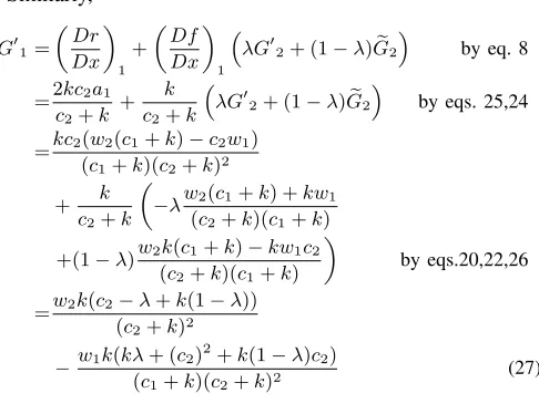
G01= Dr Dx 1 + Df Dx 1
λG02+ (1−λ)Ge2
by eq. 8
=2kc2a1
c2+k
+ k
c2+k
λG02+ (1−λ)Ge2
by eqs. 25,24
=kc2(w2(c1+k)−c2w1) (c1+k)(c2+k)2
+ k
c2+k
−λw2(c1+k) +kw1
(c2+k)(c1+k)
+(1−λ)w2k(c1+k)−kw1c2 (c2+k)(c1+k)
by eqs.20,22,26
=w2k(c2−λ+k(1−λ)) (c2+k)2
−w1k(kλ+ (c2)
2
+k(1−λ)c2)
(c1+k)(c2+k)2
(27)
IV. DIVERGENCEEXAMPLES FORVGLANDDHP
ALGORITHMS
We now have the whole trajectory and the terms Ge andG0
written algebraically, so that we can next analyse the VGL(λ) weight update for divergence.
The VGL(λ) weight update (eq. 7) combined with Ωt=1 gives
∆wi=α
X
t
∂Ge ∂wi
!
t
(G0t−Get) (28a)
=α(G0i−Gei) (fori∈ {1,2}, by eq. 14)
⇒
∆w1
∆w2
=α G
0
1−Ge1 G02−Ge2
! =αA w1 w2 (28b)
whereAis a2×2matrix with elements found by subtracting equations 21 and 22 from equations 27 and 26, respectively, giving,
A= −
k(kλ+(c2)2+k(1−λ)c2)
(c1+k)(c2+k)2 − k
(c1+k)
k(c2+k−λ(k+1))
(c2+k)2 k(c2−1)
(c2+k)(c1+k)
−1−k
(c2+k)
!
(29)
Equation 28b is the VGL(λ) weight update written as a single dynamic system of just twovariables, i.e. a shortened weight vector, w~ = (w1, w2)T. For this shortened weight
vector, w~, by looking at the right-hand sides of the sequence of equations from eq. 28a to eq. 28b, we can conclude that
X
t
∂Ge ∂ ~w
!
t
(G0t−Get) =A ~w (30)
To add further complexity to the system, in order to achieve the desired divergence, we next define these two weights to be a linear function of twootherweights,~p= (p1, p2)T, such
that the shortened weight vector is given by w~ =F ~p, where
F is a2×2constant real matrix. The VGL(λ) weight update
equation can now be recalculated for these new weights, as follows:
∆p~=αX
t
∂Ge ∂~p
!
t
(G0t−Get) by eq. 7 andΩt=1
=αX
t
∂ ~w ∂~p
∂Ge ∂ ~w
!
t
(G0t−Get) by chain rule
=α∂ ~w ∂~p
X
t
∂Ge ∂ ~w
!
t
(G0t−Get) since independent oft
=α∂ ~w
∂~pA ~w by eq. 30
=α(FTAF)~p. byw~=F ~pand ∂ ~w ∂~p =
∂(F ~p)
∂~p =F
T
(31)
The optimal actions a0 = a1 = 0 would be achieved by ~
p=~0. To produce a divergence example, we want to ensure that ~pdoes notconverge to~0.
Takingα >0to be sufficiently small, then the weight vector
~
p evolves according to a continuous-time linear dynamic system given by eq. 31, and this system is stable if and only if the matrix product FTAF is “stable” (i.e. if the real part of every eigenvalue of this matrix product is negative).
Choosing λ = 0 and c1 = c2 = k = 0.01 gives A =
−0.75 0.5
−24.75 −50.5
(by equation 29). Choosing F =
10 1
−1 −1
makes FTAF =
117.0 −38.25 189.0 −27.0
which has
eigenvalues45±45.22i. Since the real parts of these eigen-values are positive, eq. 31 will diverge for VGL(0) (i.e. DHP). In an extended analysis, we found that these parameters also cause VGL(0) to diverge when the Ωt matrices are included according to equation 10 (see the Appendix for further details). Since GDHP is a linear combination of DHP, which we have proven to diverge, and TD(0) (which we prove to diverge below), it follows that GDHP can diverge with a greedy policy too.
Also, perhaps surprisingly, it is possible to get instability with VGL(1). Choosing c2 = k = 0.01, c1 = 0.99 gives A =
−0.2625 −24.75
−0.495 −50.5
. Choosing F =
−1 −1
.2 .02
makes FTAF =
2.7665 0.1295 4.4954 0.2222
which has two positive
real eigenvalues. Therefore this VGL(1) system diverges. Diverging weights are shown for the VGL(0) and VGL(1) algorithms in Figure 1, with a learning rate of α = 10−6. Both experiments (and all subsequent experiments in this paper) used a starting weight vector of (p1, p2, w3, w4) =
(5.23∗10−5,8.53∗10−5,0,0), which is based upon a principal eigenvector of the FTAF matrix found to make VGL(1) diverge.
[image:6.612.56.299.75.262.2]1e-08 1e-06 0.0001 0.01 1 100 10000
1 10 100 1000 10000 100000 1e+06 1e+07
|
~p
|
Iterations VGL(0)/DHP
[image:7.612.39.295.61.176.2]VGL(1)
Fig. 1. Divergence for VGL(0) (i.e. DHP) and VGL(1) using the learning
parameters described in section IV and a learning rate ofα= 10−6.
1e-10 1e-09 1e-08 1e-07 1e-06 1e-05 0.0001 0.001 0.01 0.1
1 10 100 1000 10000 100000 1e+06 1e+07
|
~p
|
[image:7.612.308.542.163.408.2]Iterations VGLΩ(1)
Fig. 2. Convergence for VGLΩ(1) using the same parameters that caused
VGL(1) to diverge, and α= 10−3. This algorithm demonstrates that itis
possible to have proven convergence for a critic learning algorithm with a greedy policy and general function approximation.
V. DIVERGENCE RESULTS FORTD(λ), SARSA(λ)AND
HDP
To satisfy the requirement for exploration in TD(λ)-based algorithms, we supplemented the greedy policies (eqs. 16 & 17) with a small amount of stochastic Gaussian noise with zero mean and variance 0.0001. This Gaussian noise was necessary, since it is well known that these classic RL algorithms must be supplemented with some form of exploration. This is the classic “exploration versus exploitation” dilemma. Without exploration, these algorithms do not converge to an optimal policy, in general. Specific examples of converging to the wrong policy without exploration are given by [17, sec. IV.H] and [15, appendix B].
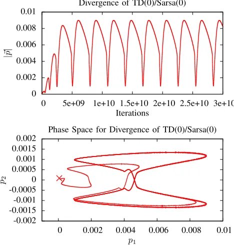
To achieve divergence of these algorithms with the noisy greedy policy, we used exactly the same learning and environ-ment constants as used for the VGL(0) and VGL(1) divergence experiments. These choices of parameters, with the stochastic noise added to the greedy policy, made TD(0) and TD(1) diverge respectively, as shown in figures 3 and 4. Hence HDP diverges too, since this is equivalent to TD(0) with the given policy.
Although these divergence results for the TD(λ) based algo-rithms were only found empirically, as opposed to the results for the previous sections which were first found analytically, these results do still have value. Firstly, source code for the em-pirical experiments used here is provided by [18, in ancillary files], so the empirical results should be entirely replicable. Secondly, an insight into why the divergence parameters for
VGL were sufficient to make the TD( ) based algorithms diverge too is because TD with stochastic exploration can be understood to be an approximation to a stochastic version of VGL(λ), so we wouldexpecta divergence example for VGL to cause divergence for TD(λ) too.
Without the stochastic noise added to the greedy policy, these examples would not diverge, but instead converge to a sub-optimal policy, which is also considered a failure.
0 0.002 0.004 0.006 0.008 0.01
0 5e+09 1e+10 1.5e+10 2e+10 2.5e+10 3e+10
|
~p
|
Iterations
Divergence of TD(0)/Sarsa(0)
-0.002 -0.0015 -0.001 -0.0005 0 0.0005 0.001 0.0015 0.002
0 0.002 0.004 0.006 0.008 0.01 p2
p1
Phase Space for Divergence of TD(0)/Sarsa(0)
Fig. 3. Divergence for TD(0) and Sarsa(0) generated with the diverging
parameters described in section V, and a learning rate ofα= 10−6. The
upper graph shows progress of|~p|versus iterations. The lower graph shows the
corresponding evolution of the weight vector components(p1, p2)in phase
space. This phase curvestartsclose to the origin (at the ‘X’), and finishes off in a limit cycle.(Errata, 2015-09): The phase space graph is plotted incorrectly. See Fig. 9.2 of first author’s phd thesis for a correction.
1e-08 1e-06 0.0001 0.01 1
1 100 10000 1e+06 1e+08 1e+10
|
~p
|
Iterations TD(1)/Sarsa(1)
Fig. 4. Divergence for TD(1) and Sarsa(1) generated with the diverging
parameters described in section V, and a learning rate ofα= 10−6.
A. Divergence results for Sarsa(λ)
We next prove divergence for Sarsa(λ) by choosing a function approximator for Qe that makes the Sarsa(λ) weight
[image:7.612.40.297.221.339.2] [image:7.612.310.533.510.621.2]Sarsa(λ) is designed to work with an arbitrary function approximator for Qe(~x, ~a, ~w). We will define our Qe function
exactly by Eq. 2. Rearranging eq. 6 gives
Qλ
t−rt
γ
=λQλt+1+ (1−λ)Qet+1
=λQλt+1+ (1−λ)(rt+1+γVet+2) by eq. 2
=rt+1+λ(Qλt+1−rt+1) + (1−λ)(γVet+2)
=rt+1+γ λ
Qλ
t+1−rt+1
γ !
+ (1−λ)Vet+2 !
(32)
From this we can see that Qλt−rt
γ
obeys the same
recursion equation as Rλ, and they have the same endpoint (since both are zero at a terminal state), from which we can conclude (e.g. by comparing recursion equations 32 and 4) that
Qλ t−rt
γ
≡Rλt+1
⇒Qλt=rt+γRλt+1
Substituting this into the Sarsa(λ) weight update (eq. 5), with eq. 2, and simplifying gives
∆w~ =αX
t
∂(rt+γVe(~xt+1, ~w)) ∂ ~w
!
t
(rt
+γRλt+1−(rt+γVet+1)
=αX
t
γ ∂Ve ∂ ~w
!
t+1
γ(Rλt+1−Vet+1)
=αγ2X
t>0 ∂Ve ∂ ~w
!
t
(Rλt−Vet)
which is identical to TD(λ) but with summation overt now excluding t = 0, and with an extra constant factor, γ2. The divergence example we derived above used γ = 1, and had no weight update term for t = 0, so uses an identical weight update. Therefore this particular choice of function approximator forQe and problem definition causes divergence
for Sarsa(λ) (with bothλ= 1andλ= 0). VI. CONCLUSIONS
We have shown that under a value-iteration scheme, i.e. using a greedy policy, all of the RL algorithms have been made to diverge, and all but one of the VGL algorithms have been made to diverge. The algorithm we found that didn’t diverge was VGLΩ(1) withΩtas defined by eq. 10, which is proven to converge by [9] and [15] under these conditions.
These are new divergence results for TD(0), Sarsa(0), TD(1) and Sarsa(1), in that previous examples of divergence have only been for TD(0) and for non-greedy policies [19], [20], [11]. The divergences we achieved for TD(1) and Sarsa(1) were only possible because of the use of a greedy policy (or equivalently, value-iteration).
A conclusion of this work is that the diverging algo-rithms considered cannot currently be reliably used for value-iteration, and instead can only be used under some form of
policy iteration if provable convergence is required. However there are some distinct advantages of value-iteration over policy-iteration. Value-iteration using a greedy policy can be faster than using an actor-critic architecture. Also policy iteration does provably converge in some cases [21], but the necessary conditions are thought to apply only when the function approximator forVe islinearin the same features of
the state vector that the function approximator for the policy uses as input (see footnote 1 of [21]).
The divergence results of this paper were derived for quadratic critic functions, as this was the situation that allowed for easiest analysis to derive concrete divergence examples. We assume that similar divergence results will exist for neural network based critic functions, since neural networks are more complex structures that should allow for more possibilities for divergence situations similar to our simple example here. In our experience, divergence often does occur when using a greedy policy with a neural network critic, but these situations are harder to analyse and make replicable. In this situation, we speculate that a second order Taylor series expansion of the neural network could be made about the fixed point of the learning process, and locally this approximation could be behaving very similarly to the quadratic functions we have used in this paper.
It is hoped that the specific divergence examples of this paper will provide a better understanding of how value-iteration can diverge, and help motivate research to understand and prevent it. We believe that the value-gradient analysis that produced the converging algorithm of Figure 2 by [9] could be helpful for reinforcement learning research, since this is a critic learning algorithm that does have convergence guarantees under a greedy policy with general function ap-proximation.
APPENDIX
In this appendix we give the extension analysis that was used to determine that VGLΩ(0) (i.e. VGL(0) with the Ωt matrix of eq. 10) could be made to diverge. We also include an analysis that shows VGLΩ(1)will converge in the experiment of this paper for any choice of experimental constants.
To construct the Ωt matrix of eq. 10, first we note that differentiating equation 11a gives ∂f∂a
t= 1, fort∈ {0,1}. And differentiating equation 15 gives
∂2
e Q ∂~a∂~a
!
t
=−2(ct+1+k) for t∈ {0,1}.
Hence, by equation 10,
Ωt=
(
1/(2(ct+k)) for t∈ {1,2}
0 for t= 0.
The VGL(λ) weight update can be re-derived using this newΩtmatrix. Following the method that was used to derive equations 28a to 30, but starting with this newΩtmatrix, gives
X
t
∂Ge ∂ ~w
!
t
Ωt(G0t−Get) =αDA
w1 w2
whereD= 2(c1+k)
0 1 2(c2+k)
andAis given by equation
29. Then, definingw~ =F ~pfor a constant matrixF(as done in section IV), and following the method that was used to derive eq. 31, we would derive the VGL(λ) weight update for the weight vector ~pas
∆p~=α(FTDAF)~p.
As before, this system will converge for sufficiently small α
if and only if the product FTDAF is “stable”, i.e. if the real parts of the eigenvalues are negative.
A. Divergence of VGLΩ(0)
Choosing the same parameters that made VGL(0) diverge,
i.e. c1=c2=k= 0.01, givesD=
25 0 0 25
. SinceD is a positive multiple of the identity matrix, its presence will not affect the stability of the productFTDAF, so the system for
~
pwill still be unstable, and diverge, just as it did for VGL(0).
B. Convergence of VGLΩ(1)
When VGLΩ(1) is used, convergence can be proven for any choice of parameters as follows: When λ= 1, the A matrix of eq. 29 reduces to2
A= −
k(k+(c2)2)
(c1+k)(c2+k)2 − k
(c1+k)
k(c2−1)
(c2+k)2 k(c2−1)
(c2+k)(c1+k)
−1−k
(c2+k)
!
=2 −
k(k+(c2)2)
(c2+k)2 −k
k(c2−1)
(c2+k) k(c2−1)
(c2+k) −1−k
! D
=2E
−k(k+ (c2)2+ (c2+k)2) k(c2−1) k(c2−1) −1−k
ED
where E =
1 (c2+k) 0
0 1
. Hence the matrix product
FTDAF can now be written as 2FTDEBEDF where
B =
−k(k+ (c2)2+ (c2+k)2) k(c2−1) k(c2−1) −1−k
. This new
product is real and symmetrical (as we would expect it to be for true gradient descent), hence it has real eigenvalues. For any c2 > 0 and k > 0, the central matrix B has a
negative trace, and a determinant equal tok(k+ 2)(k+c2)2,
which is positive. HenceB has two negative real eigenvalues. Therefore, assumingF is a full-rank matrix, the matrix prod-uct 2FTDEBEDF must be negative definite, and therefore stable, and thus the dynamic system for ~pwill converge.
REFERENCES
[1] F.-Y. Wang, H. Zhang, and D. Liu, “Adaptive dynamic programming:
An introduction,”IEEE Computational Intelligence Magazine, vol. 4,
no. 2, pp. 39–47, 2009.
[2] R. S. Sutton and A. G. Barto,Reinforcement Learning: An Introduction. Cambridge, Massachussetts, USA: The MIT Press, 1998.
[3] R. E. Bellman,Dynamic Programming. Princeton, NJ, USA: Princeton
University Press, 1957.
2This version of this document contains a fix to the following equations - the
constant factor 2 was missing from the version published in the proceedings of IJCNN12.
[4] G. Rummery and M. Niranjan, “On-line q-learning using
connection-ist systems,” Tech. Rep. Technical Report CUED/F-INFENG/TR 166,
Cambridge University Engineering Department, 1994.
[5] R. S. Sutton, “Learning to predict by the methods of temporal
differ-ences,”Machine Learning, vol. 3, pp. 9–44, 1988.
[6] P. J. Werbos, “Approximating dynamic programming for real-time control and neural modeling.” inHandbook of Intelligent Control, D. A. White and D. A. Sofge, Eds. New York: Van Nostrand Reinhold, 1992, ch. 13, pp. 493–525.
[7] D. Prokhorov and D. Wunsch, “Adaptive critic designs,”IEEE
Transac-tions on Neural Networks, vol. 8, no. 5, pp. 997–1007, 1997. [8] S. Ferrari and R. F. Stengel, “Model-based adaptive critic designs,” in
Handbook of learning and approximate dynamic programming, J. Si,
A. Barto, W. Powell, and D. Wunsch, Eds. New York: Wiley-IEEE
Press, 2004, pp. 65–96.
[9] M. Fairbank and E. Alonso, “The local optimality of reinforcement learning by value gradients, and its relationship to policy gradient
learning,” CoRR, vol. abs/1101.0428, 2011. [Online]. Available:
http://arxiv.org/abs/1101.0428
[10] ——, “Value-gradient learning,” inProceedings of the IEEE
Interna-tional Joint Conference on Neural Networks 2012 (IJCNN’12). IEEE Press, June 2012, pp. 3062–3069.
[11] J. N. Tsitsiklis and B. Van Roy, “An analysis of temporal-difference learning with function approximation,” IEEE Transactions on Automatic Control, Tech. Rep., 1996.
[12] R. S. Sutton, H. R. Maei, D. Precup, S. Bhatnagar, D. Silver, C. Szepesv´ari, and E. Wiewiora, “Fast gradient-descent methods for temporal-difference learning with linear function approximation,” in
Proceedings of the 26th Annual International Conference on Machine Learning, ser. ICML ’09. New York, NY, USA: ACM, 2009, pp. 993– 1000.
[13] H. Maei, C. Szepesv´ari, S. Bhatnager, D. Precup, D. Silver, and R. Sut-ton, “Convergent temporal-difference learning with arbitrary smooth
function approximation,” inAdvances in Neural Information Processing
Systems (NIPS’09). MIT Press, 2009.
[14] P. J. Werbos, “Stable adaptive control using new critic designs,”eprint arXiv:adap-org/9810001, 1998.
[15] M. Fairbank, “Reinforcement learning by value gradients,”CoRR, vol.
abs/0803.3539, 2008. [Online]. Available: http://arxiv.org/abs/0803.3539 [16] C. J. C. H. Watkins, “Learning from delayed rewards,” Ph.D.
disserta-tion, Cambridge University, 1989.
[17] M. Fairbank and E. Alonso, “A comparison of learning speed and ability
to cope without exploration between DHP and TD(0),” inProceedings
of the IEEE International Joint Conference on Neural Networks 2012 (IJCNN’12). IEEE Press, June 2012, pp. 1478–1485.
[18] ——, “The divergence of reinforcement learning algorithms with value-iteration and function approximation,”eprint arXiv:1107.4606, 2011. [19] L. C. Baird, “Residual algorithms: Reinforcement learning with function
approximation,” in International Conference on Machine Learning,
1995, pp. 30–37.
[20] J. N. Tsitsiklis and B. Van Roy, “Feature-based methods for large scale
dynamic programming,”Machine Learning, vol. 22, no. 1-3, pp. 59–94,
1996.
[21] R. S. Sutton, D. Mcallester, S. Singh, and Y. Mansour, “Policy gradient methods for reinforcement learning with function approximation,” in