Comparing Policy Gradient and Value Function
Based Reinforcement Learning Methods in
Simulated Electrical Power Trade
Richard Lincoln, Stuart Galloway, Bruce Stephen, Member, IEEE Graeme Burt, Member, IEEE
Abstract—In electrical power engineering, reinforcement learn-ing algorithms can be used to model the strategies of electricity market participants. However, traditional value function based reinforcement learning algorithms suffer from convergence issues when used with value function approximators. Function approx-imation is required in this domain to capture the characteristics of the complex and continuous multivariate problem space. The contribution of this paper is the comparison of policy gradient reinforcement learning methods, using artificial neural networks for policy function approximation, with traditional value function based methods in simulations of electricity trade. The methods are compared using an AC optimal power flow based power exchange auction market model and a reference electric power system model.
Index Terms—Artificial intelligence, game theory, gradient methods, learning control systems, neural network applications, power system economics.
I. INTRODUCTION
W
ITH growing world population comes increasing de-mand for energy and with it, dede-mand for the fuels used to generate electricity. Competitive markets have an important role to play in the management of this demand and the subsequent price paid for electricity by consumers. Market designs for electricity are unique among commodity markets and new architectures are expensive and risky to implement. The importance of electricity to society makes it impractical to experiment with radical changes to trading arrangements on real systems. As an alternative it is possible to study abstract mathematical models of markets with sets of appropriate simplifying approximations and assumptions ap-plied. Market architecture characteristics and the consequences of proposed changes can be established by simulating the models as digital computer programs. Competition between participants is fundamental to all markets, but the strategies of human participants are a challenge to model mathematically.Unsupervised reinforcement learning algorithms from the field of artificial intelligence can be used to represent adaptive behaviour in competing players [1] and have been shown to be capable of learning highly complex strategies [2]. Individuals participating in an electricity market (be they representing generating companies, load serving entities or firms of traders)
This research was funded by the United Kingdom Engineering and Physical Research Council under grant GR/T28836/01.
R. Lincoln, S. Galloway, B. Stephen and G. Burt are with the Department of Electronic and Electrical Engineering, The University of Strathclyde, Glasgow, Scotland.
must utilise voluminous multi-dimensional data to their ad-vantage. Data may be noisy, sparse, corrupt, have a degree of uncertainty (e.g. demand forecasts) or be hidden from the participant (e.g. competitor bids). Reinforcement learning algorithms must also be capable of operating with data of this kind if they are to successfully model participant strategies.
Traditional reinforcement learning algorithms attempt to learn a function that returns the long-term expected reward of each action available in a given state. Generalisation tech-niques can be used to approximate this value function and allow continuous mutli-variate state and action spaces to be used. However, it has been found that the greedy updates used with most techniques can prevent these algorithms from generalising even in simple problems [3]–[5].
Policy gradient algorithms are an alternative form of rein-forcement learning method that do not learn a value function, but adjust an agent’s policy directly [6]. They can be used with function approximation techniques without suffering from the problems that mar value function based methods. They have been successfully applied in several types of operational setting, including robotic control [7], financial trading [8], [9] and network routing [10], but they have not been previously applied in simulations of competitive electricity trade.
In this paper, two policy gradient algorithms are compared with one value-function based method and two variants of the popular Roth-Erev technique [11]. A power exchange auction market model is used to facilitate trade between learning agents and AC optimal power flow solutions are used to clear submitted offers. The IEEE Reliability Test System provides a reference electric power system model that provides dynamic load profiles and a realistic generation mix with associated costs [12]. Learning agents are each endowed with roughly equivalent portfolios of generating stock. The agents can mark-up offer prices above marginal cost and withhold generating capacity within specified limits. The algorithms are compared in their profitability over a simulated year of trade.
II. REINFORCEMENTLEARNING
Reinforcement learning is learning from reward by map-ping situations to actions when interacting with an uncertain environment [13]. In the classical model of agent-environment interaction, at each time stept in a sequence of discrete time steps t= 1,2,3. . . an agent receives as input some form of the environment’s state st∈S, whereS is the set of possible
states. From a set of actions A(st) available to the agent in state st the agent selects an action at and performs it in its
environment. The environment enters a new state st+1 in the next time step and the agent receives a scalar numerical reward rt+1∈Rin part as a result of its action. The agent then adjusts its policy for selecting actions by learning from the state representationst, the chosen actionat and the reinforcement
signalrt+1 before beginning its next interaction.
Traditional reinforcement learning methods, such as Q-learning [14] or Sarsa [15], attempt to learn an action-value functionQ(st, at)that returns the long term expected reward
vst,at
t for taking action at in state st. If a discrete number
of states ns and actionsna are defined, these values may be
stored in a look-up table of the form:
a1 a2 ana s1 v1,1 v1,2 · · · v1,na s2 v2,1 . .. ...
..
. . .. ...
sns vns,1 · · · · · · vns,na
(1)
In Q-learning the values are updated after each interaction according to the equation
Q(st, at) =Q(st, at)+α
rt+1+γmax
a Q(st+1, a)−Q(st, at)
(2) where γ is a discount factor, with 0 ≤γ ≤ 1 that prevents values from going unbounded and represents reduced trust in the reward rt as discrete time t increases. The learning rate
α, where0 ≤α≤1, controls how much attention is paid to new data when updating.
A balance between exploration of the environment and exploitation of past experience must be struck when selecting actions. The ǫ-greedy approach to action selection is defined by a randomness parameter ǫ, where0≤ǫ≤1, and a decay parameter d [16]. A random number xr where 0 ≤ xr ≤ 1
is drawn for each selection. If xr < ǫ then a random action
is selected, otherwise the perceived optimal action is chosen. After each selection the randomness is attenuated byd.
Enumerating high-dimensional state and action spaces can result in impractical memory requirements in all but the simplest of problems [1]. Function approximation techniques, such as artificial neural networks [17], can be used to ap-proximate the value function and allow these methods to be applied to problems with multi-dimensional and continuous environments [18]. However, it has been found that updates from greedy action selections can cause methods using this technique to fail to generalise [3]–[5].
Policy gradient reinforcement learning methods learn a
policy function that returns an action given the current
per-ceived state of the environment [6]. Small incremental changes
are made to the parameter vector θ of a policy function approximator (connection weights in the case of an artificial neural network) in the direction of steepest ascent of some policy performance measureY with respect to the parameters
θt+1=θt+α
∂Y ∂θt
(3)
where α is again a positive definite step size learning rate. Policy gradient methods are differentiated largely by the tech-niques used to obtain an estimate of the gradient∂Y /∂θ. Some of the most successful real-world robotics results [7], [19] have been yielded by likelihood ratio methods such as Williams’ REINFORCE[20] and natural policy gradient methods, such as the Episodic Natural Actor-Critic (ENAC) [21]. For a concise overview of these methods the interested reader is referred to [22].
A relatively simple reinforcement learning method, pro-posed by Alvin E. Roth and Ido Erev [11], has received considerable attention from the agent based electricity market simulation community. The algorithm is based on empirical results obtained by observing how humans learn decision making strategies in games against multiple strategic players. It learns a policy in which the state of the environment is ignored and each action a is associated with a single value q that is the agent’s propensity for selecting it. After each interaction the propensity for the previous action, that resulted in the rewardrt, is adjusted by an experimentation parameter
ǫ and all other action propensities are adjusted by a small proportion of their current value.
Two shortcomings of the original Roth-Erev algorithm were identified in [23] and a modified formulation was proposed. Under this variant, after selecting actiona′ in interactiontthe
propensity to select actionafor interactiont+ 1is:
qa(t+ 1) =
(
(1−φ)qa(t) +rt(1−ǫ), a=a′
(1−φ)qa(t) +qa(t)(A−ǫ1), a6=a′ (4)
where A is the total number of feasible actions and φ is the recency parameter. The recency, or forgetting parameter degrades the propensities for all actions and prevents propen-sity values from going unbounded. It is intended to represent the tendency for players to forget older action choices and to prioritise more recent experience. The experimentation parameter prevents the probability of choosing an action from going to zero and encourages exploration of the action space. This paper proposes a new stateful variant of the Roth-Erev method. Instead of assuming only one state and maintaining only one row of propensities, a multi-row table with one row per environment state, as with Q-learning, is used. Action propensity values are still updated according to equation 4, but it is the values in the row associated with the previous state that are modified during the learning step. The method allows differentiation between states, but can increase the number of propensity values that require updating.
III. RELATEDWORK
expert knowledge and intuition, and were implemented as basic trading rules [24]–[27]. Successive publications from the London Business School illustrate a trend in the field towards more complex algorithms and improved behavioural models [28], [29].
More recently, unsupervised reinforcement learning algo-rithms from the field of artificial intelligence have been used in energy market research [30]. Variations on the Q-learning technique have been used to study congestion management schemes [31], combined electricity and gas markets [32] and emissions allowance trading [33]. The Roth-Erev method has been used to study market power [23], the Italian wholesale electricity market [34], cross-holdings1[35], and interrelation-ships between contracts markets and balancing markets [36], [37].
Policy gradient reinforcement learning methods have not previously been used in agent-based electricity market re-search, but have been successfully applied in other laboratory [6] and operational settings [7], [10]. In [8] and [9] a recurrent gradient method was used to optimise financial investment performance without price forecasting and in [38] a modified version of REINFORCE is used to simulate a marketplace for grid computing resources.
IV. MODELLINGELECTRICITYTRADE
In this paper a power exchange auction market model is used to provide an electricity trading environment for comparing reinforcement learning algorithms. It is based on the SmartMarket model that is provided with MATPOWER [39] and was developed for the PowerWeb project at Cornell University. Market participants are modelled using software agents from PyBrain [40] that use reinforcement learning algorithms to adjust their behaviour. Their interaction with the market is coordinated in multi-agent simulations, the structure of which is derived from PyBrain’s single player design. The multi-agent system consists of discrete and continuous market
environments, specific tasks for agents and modules that are
used for policy function approximation and storing state-action values or action propensities.
A. Power Exchange Auction Market
In each trading period the auction accepts offers to sell blocks of capacity from participating agents. A double-sided auction, in which bids to buy blocks of power may be submitted by agents associated with dispatchable loads, is also available, but this feature is not used. Valid offers for each generator are sorted into non-decreasing order with respect to price and converted into corresponding generator capacities and piecewise linear cost functions. The newly configured units form a unit-decommitment optimal power flow problem [39], the solution to which provides generator set-points and nodal marginal prices that are used to determine the proportion of each offer block that should be cleared and the associated clearing price. The cleared offers determine each agent’s revenue and hence the profit that is used as the reward signal.
1Cross-holdings occur when one publicly traded firm owns stock in another publicly traded firm.
A nodal marginal pricing scheme is used in which the price of each offer is cleared at the value of the Lagrangian multiplier on the power balance constraint for the bus at which the offer’s generator is connected.
B. Market Environments for Agents
Each agent has a portfolio of ng generators associated
with their local environment. Each environment is responsible for (i) returning a vector representation of its current state and (ii) accepting an action vector which transforms the environment into a new state.
1) Discrete Market Environment: For agents using the
Q-learning or Roth-Erev methods, an environment with ns
discrete states and na discrete action possibilities is defined.
The environment produces a state s, where s ∈ Z+ and
0 ≤ s < ns, at each simulation step and accepts an action
a, where a ∈ Z+ and 0 ≤ a < n
a. To prevent state
space enumeration from exceeding memory limits the discrete states are derived only from the current total system demand d=P
Pd, where Pd is the vector of active power demand at
each bus. Informally, the state space isns states between the
minimum and maximum demand and the current state st is
the index of the state to which the present demand,d, relates. The action space for a discrete environment is defined by a vector m, where 0 ≤ mi ≤ 100, of percentage markups
on marginal cost with length nm, a vector w, where 0 ≤
wi ≤ 100, of percentage capacity withholds with length nw
and a scalar number of offers no, where no ∈ Z+, to be
submitted for each generator associated with the environment. Each offer relates to one price-quantity block, where the price is the marginal cost of the associated generator marked up by mi percent and the quantity is pg/no, where pg is the rated
output of the associated generator, with wi percent withheld.
Increasingno provides greater flexibility with regards to how
capacity is sold, allowing some capacity to be offered at a low price, ensuring dispatch, and for the remainder to be marked up further, risking non-dispatch for the chance of greater profit.
2) Continuous Market Environment: For agents operating
policy gradient learning algorithms a continuous environment is defined. It outputs a state vector s, where si ∈ R, and
accepts an action vector a, where ai ∈ R. Scalar variables
mu andwu define the upper limit on the percentage markups
on marginal cost and the upper limit on the percentage of capacity that can be withheld, respectively. Again,nodefines
the number of offers to be submitted for each generator associated with the environment.
The state vector can be any set of variables from the power system or market model, e.g. bus voltages, branch power flows, generator limit Lagrangian multipliers. Each element of the vector provides one input to the neural network used for policy function approximation.
The action vector a has length 2ngno. Element ai, where
0 ≤ ai ≤ mu, corresponds to the percentage price markup
andai+1, where0≤ai+1≤wu, to the percentage of capacity
to withhold for the (i/2)th offer from the agent, where i =
C. Agent Tasks
To allow alternative goals (such a profit maximisation or meeting some target level for plant utilisation) to be associated with a single type of environment, an agent does not interact directly with the environment, but through a particular task [40]. Using some measure of risk adjusted return (as in [8]) might be of interest in the context of simulated electricity trade and this would simply involve the definition of a new task and would not require any modification of the environment.
A task defines the reward returned to the agent and thus defines the agent’s purpose. For all simulations in this paper, the goal of each agent is to maximise direct financial profit. Rewards are defined as the sum of earnings from the previous periodt, as determined by the difference between the revenue from cleared offers and generator marginal costs at their total cleared quantity.
Given a task, an agent may have a restricted view of the environment or be able to only perform certain actions. Thus a task adjusts the state vector before it is passed to the agent and makes adjustments to the action vector before it is passed to the environment. Agents operating policy-gradient learning methods approximate their policy functions using artificial neural networks that are presented with input vector x of length ns where xi ∈ R. The state vector from the
environment may consist of values that differ greatly in their relative magnitude. To ensure that all values have a similar influence on the agent’s policy, the task produces a normalised vector, with −1 ≤ xi ≤ 1, for input to the policy function
approximator. To accomplish this, vectors of lower and upper sensor limits are defined, sl andsu respectively, and used to
calculate the normalised input vector
x= 2
s
−sl
su−sl
−1. (5)
To produce an output vector y, where −1 ≤ yi ≤ 1,
nodes that implement a hyperbolic tangent activation function are used in the output layer of the artificial neural network. Outputs in this range can be denormalized to provide values for markup and capacity withhold that are valid for the associated generator if vectors of lower and upper action limits, al and
au respectively, are defined. The output and the limit vectors
are combined to produce an action vector
a=
y+ 1
2
(au−al) +al (6)
where 0 ≤ ai ≤ mu and 0 ≤ ai+1 ≤ wu for i =
0,2,4, . . . ,2ngno.
D. Participant Agents
Each agent is defined as an entity capable of producing an actiona based on previous observations of its environments and is associated with a module, a learner, a dataset and an
explorer.
The module is used to determine the agent’s policy for action selection and returns an action vectorawhen activated with observation s. For Q-learning the module is a ns×na
table where each element vst,at
t is the value in state st
associated with selecting action at at simulation step t. For
a standard Roth-Erev learner, the table has one row that stores the propensity for selection of each action.
The module for policy gradient methods is a multi-layer feed-forward artificial neural network that outputs a vector a when presented with an observation vectors.
The learner can be any reinforcement learning algorithm that modifies the values/propensities/parameters of the module to increase expected future reward. The dataset stores state-action-reward triples for each interaction between the agent and its environment. The stored history is used by learners when computing updates to the module.
Each learner is associated with an explorer that adds a de-gree of exploration to the agents action selection by returning an explorative actionaewhen activated with the current state
s and action afrom the module. Softmax and ǫ-greedy [13] explorers are implemented for discrete action spaces. Policy gradient methods use an additional module that adds Gaussian noise to the output of the neural network. The explorer has a parameter σ that relates to the standard deviation of the Gaussian distribution.
V. IEEE RELIABILITYTESTSYSTEMSIMULATION
Learning methods are compared by repeating the same simulation of competitive electricity trade and switching the type of algorithm used by the competing agents. The IEEE Reliability Test System (RTS) provides a reference electric power system model, hourly load profiles for a whole year and a realistic generation mix with costs. Each agent interacts with the market once for each hour of the simulated year, submitting offers for each of the generators in its portfolio and this is then repeated for each of the learning algorithms.
The model has 24 bus locations that are connected by 32 transmission lines, 4 transformers and 2 underground cables. The transformers tie together a 230kV area and a 138kV area. The original model has 32 generators of 9 different types with a total capacity of 3.45GW. To reduce the size of the discrete action domain, five 12MW and four 20MW generators are removed. This is a minor alteration as their combined capacity is only 4.1% of the original total generation capacity and the remaining capacity is still sufficient to meet demand. To further reduce action space sizes all generators of the same type at the same bus are aggregated into one unit. This may be considered to be the representation of each individual power station in the market, rather than each synchronous machine. The model has loads at 17 locations and the total demand at system peak is 2.85GW. The connectivity of branches and the location of generators and loads is illustrated in Fig. 1. This model was selected because it is well established in the electrical engineering research community, it captures important aspects of a real transmission system (such as topology and plant ratings) and it is suitably sized for repeated simulation.
Generator marginal costs are quadratic functions, of the formc(pi) =ap2i+bpi+cwherepi is the output of generator
Bus 1 Bus 2 Bus 3
Bus 4
Bus 5
Bus 6
Bus 7 Bus 8
Bus 9 Bus 10
Bus 11 Bus 12
Bus 13 Bus 14
Bus 15 Bus 16 Bus 17
Bus 18
Bus 19 Bus 20
Bus 21 Bus 22
Bus 23
Bus 24
cable
cable
A1 152 MW 2×U76
A2 152 MW
2×U76 A4 300 MW
3×U100 A3 591 MW 3×U197 A5 Synch.
Cond. A1
155 MW A2 155 MW
A1 400 MW
Nuclear A2 400 MW Nuclear
A3 300 MW Hydro, 6×U50
A4 660 MW 2×U155 1×U350
108 MW
97 MW 108
MW
74 MW
71 MW
136 MW
125 MW 171 MW 175 MW
195 MW 265 MW 194 MW
317 MW 100
MW
333 MW
181 MW 128 MW
138 kV
[image:5.612.70.282.52.365.2]230 kV
[image:5.612.76.273.428.534.2]Fig. 1. Single line diagram for the simplified IEEE Reliability Test System.
TABLE I
GENERATOR TYPES AND COST PARAMETERS FOR THE SIMPLIFIEDIEEE RELIABILITYTESTSYSTEM.
Code a b c Type
U50 0.0 0.001 0.001 Hydro
U76 0.01414 16.0811 212.308 Coal
U100 0.05267 43.6615 781.521 Oil
U155 0.00834 12.3883 382.239 Coal
U197 0.00717 48.5804 832.758 Oil
U350 0.00490 11.8495 665.109 Coal
U400 0.00021 4.4231 395.375 Nuclear
TABLE II
PORTFOLIOS OF GENERATING PLANT ENDOWED TO EACH AGENT.
Agent U50 U76 U100 U155 U197 U350 U400 Hydro Coal Oil Coal Oil Coal Nuclear
1 2× 1× 1×
2 2× 1× 1×
3 6× 3×
4 3× 2× 1×
taken from an RTS model by Georgia Tech Power Systems Control and Automation Laboratorythat assumes Coal costs of 1.5 $/MBtu2, Oil costs of 5.5 $/MBtu and Uranium costs of 0.46 $/MBtu.
The generating stock is divided into 4 portfolios that are each endowed to a learning agent. Table II shows the number
21 Btu (British thermal unit)≈1055 Joules
of generators of each type in each portfolio. The portfolios were chosen such that each agent has: a mix of base load and peaking plant, approximately the same total generation capacity, generators in different areas of the network and enough generators to produce a challenging action domain. The generator labels in Fig. 1 denote the associated agent. The synchronous condenser is associated with a passive agent that always offers 0 MW at 0 $/MWh (the unit can be dispatched to provide or absorb reactive power within its limits).
Markups on marginal cost are restricted to a maximum of 30% and discrete markups of 0, 15% or 30% are defined for value function based methods. Up to 20% of the total capacity of each generator can be withheld and discrete withholds of 0 or 20% are defined. These values were chosen so as to be similar with those used in [30] to allow the same findings to be reproduced and for existing research to be built upon. Finer discrete action definitions would allow agents to compete more closely to the margins of dispatch, but would greatly increase the size of the action space. However, initially only one offer per generator is required, but this is increased to two in order to explore the effect of increased state space size and offer flexibility.
The environment state for all algorithm tests is derived from a forecast of the total system demand for the next one hour period. The system demand follows the hourly profile from the RTS which varies according to the day of the week and the time of year. For tests of value function based methods and the Stateful Roth-Erev learning algorithm, the continuous state is divided into 3 equally sized discrete states between minimum and maximum demand that allow differentiation between low, medium and peak load.
To investigate exploitation of constraints, AC optimal power flow is used and the state vector for agents using policy gra-dient methods is optionally enhanced to combine the demand forecast with voltage constraint Lagrangian multipliers of all generator buses and the voltage magnitude at all other buses. Lagrangian multipliers are used as the voltage at generator buses is typically fixed and the multipliers indicate if the constraint is binding. Branch flows are not included in the state vector as the flow limits in the RTS are high and are typically not reached at peak demand. Generator capacity limits are binding in most states of the RTS, but the output of other generators is deemed to be hidden from an agent.
Typical parameter values, either defaults from PyBrain or inspired by the literature, are used for each of the algorithms. Learning rates are set low and exploration parameters decay slowly due to the length and complexity of each simulation. By decaying exploration parameters to a suitably low level, all algorithms converge to a stable policy by the end of the simulated year. No attempt to study parameter sensitivity if undertaken, but Q-learning is typically robust to parameter changes in simulations of this type [31]. For Q-learning α= 0.2,γ= 0.99andǫ-greedy action selection is used with ǫ = 0.9 and d = 0.999. For Roth-Erev learning ǫ = 0.55, φ = 0.3 and Boltzmann action selection [13] is used with τ= 100 andd= 0.999.
[image:5.612.47.301.560.630.2]0 2 4 6 8 10 12 14 16 18 20 22
0.0
0.2
0.4
0.6
0.8
1.0
1.2
1.4
1.6
1.8
Rew
ard
(
$
)
×104 Agent 1
Roth-Erev Q-Learning Stateful RE
0 2 4 6 8 10 12 14 16 18 20 22
Hour
0.0
0.2
0.4
0.6
0.8
1.0
1.2
1.4
1.6
1.8
Rew
ard
(
$
)
×104 Agent 4
[image:6.612.332.525.53.293.2]Roth-Erev Q-Learning Stateful RE
Fig. 2. Modified Roth-Erev compared with Stateful Roth-Erev.
weights are used for policy function approximation. The exploration parameterσfor these methods is initialised to zero and adjusted manually after each episodet such that:
σt=d(σt−1−σn) +σn (7)
where d = 0.995 is a decay parameter and σn = −0.5
specifies the value that is converged to asymtotically. Constant learning rates are used in each simulation with γ = 0.01 for REINFORCE and γ = 0.005for ENAC. Hourly trade for a year of 364 days is simulated for each algorithm.
VI. RESULTS
To compare algorithms, the average reward for each hour of the day over one simulated year is calculated for agents 1 and 4 and plotted. Results for only agents 1 and 4 are given as agents 1 and 2 have identical portfolios and agent 3’s portfolio consists mostly of Hydro plant with zero cost. When the marginal cost of a generator is zero, regardless of the percentage markup chosen, the offer price is always zero. This is a limitation of marking up prices based on a percentage of marginal cost, rather than by a fixed price value and results in passive market behaviour from agent 3 under all algorithms. Fig. 2 compares the Modified Roth-Erev method [23] with the Stateful Roth-Erev method. The plots show average re-wards for agents 1 and 4 when using Q-learning and the two Roth-Erev variants.
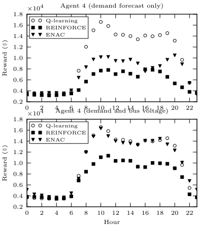
Fig. 3 and Fig. 4 compare policy gradient methods when submitting one offer per generator under two different state vector configurations. Fig. 3 concerns agent 1 and shows the average reward received for a state vector consisting solely of the demand forecast and for a combined demand forecast and bus voltage profile state vector. Fig. 4 shows average rewards for agent 4 under the same configurations. The discrete environment used by Q-learning does not use the
0 2 4 6 8 10 12 14 16 18 20 22
0.0
0.2
0.4
0.6
0.8
1.0
1.2
1.4
1.6
1.8
Rew
ard
(
$
)
×104 Agent 1 (demand forecast only)
Q-learning REINFORCE ENAC
0 2 4 6 8 10 12 14 16 18 20 22
Hour
0.0
0.2
0.4
0.6
0.8
1.0
1.2
1.4
1.6
1.8
Rew
ard
(
$
)
×104 Agent 1 (demand and bus voltage)
[image:6.612.68.264.53.293.2]Q-learning REINFORCE ENAC
Fig. 3. Average rewards for agent 1 under two state configurations.
0 2 4 6 8 10 12 14 16 18 20 22
0.2
0.4
0.6
0.8
1.0
1.2
1.4
1.6
1.8
Rew
ard
(
$
)
×104 Agent 4 (demand forecast only)
Q-learning REINFORCE ENAC
0 2 4 6 8 10 12 14 16 18 20 22
Hour
0.2
0.4
0.6
0.8
1.0
1.2
1.4
1.6
1.8
Rew
ard
(
$
)
×104 Agent 4 (demand and bus voltage)
Q-learning REINFORCE ENAC
Fig. 4. Average rewards for agent 4 under two state configurations.
voltage profile data to define its state, but results using purely the system demand are shown in all of the plots in Fig. 3 and Fig. 4 for comparison.
[image:6.612.330.525.349.574.2]0 2 4 6 8 10 12 14 16 18 20 22
0.0
0.2
0.4
0.6
0.8
1.0
1.2
1.4
Rew
ard
(
$
)
×104 Agent 1
Q-Learning ENAC
0 2 4 6 8 10 12 14 16 18 20 22
Hour
0.0
0.2
0.4
0.6
0.8
1.0
1.2
1.4
1.6
Rew
ard
(
$
)
×104 Agent 4
[image:7.612.67.264.53.294.2]Q-Learning ENAC
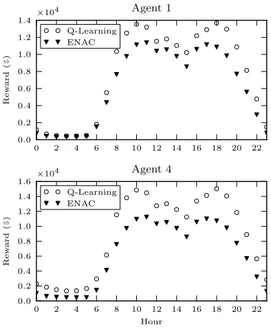
Fig. 5. Average rewards for two offers per generator.
VII. DISCUSSION
Agents with a discrete environment have 216 possible actions to choose from in each state when required to submit one offer per generator. Fig. 2 shows that, using Q-learning, the agents are able to learn an effective policy that yields increased profits using two different portfolios. The importance of util-ising environment state data in a dynamic electricity setting is illustrated by the differences in average reward received by the modified Roth-Erev method and the Stateful Roth-Erev method. The optimal action for an agent depends upon the current system load and the stateless Roth-Erev formulation is unable to interpret this. The Stateful Roth-Erev method can be seen to achieve approximately the same performance as Q-learning.
Including bus voltage constraint data in the state for a dis-crete environment would result in a state space of impractical size, but including it in a continuous environment was straight-forward. Fig. 3 and Fig. 4 show that ENAC achieves greater profits when presented with a combined demand forecast and bus voltage state vector. REINFORCE performs less well than ENAC, but also shows improvement over the pure demand forecast case. ENAC achieves equivalent, but not greater performance than Q-learning in all periods of the trading day when using the voltage data. It is not able to use the additional state information to achieve any advantage over Q-learning, but it does learn a profitable policy.
Changing the number of offers that are required to be submitted for each generator from 1 to 2, increases the number of discrete action possibilities in each state to 46,656. Fig. 5 shows that Q-learning is still able to achieve a similar level of reward as under the one offer case. The profitability for both methods is degraded, but ENAC receives significantly lower average reward when required to produce a larger action vector and is not able to use the increased flexibility in its offer
structure to any advantage.
VIII. CONCLUSION
Policy gradient methods are found to be a valid option for modelling the strategies of electricity market participants. However, in this paper they have been outperformed by a traditional action-value function algorithm in all of the sim-ulations. No evidence has been found to suggest that policy gradient methods can exploit complex constraints in a power system model. However, they have been shown to improve in performance when operating with a richer state vector that includes bus voltage level and voltage constraint information. Some limitations of the standard Roth-Erev method in an dynamic environment have been found and an alternative configuration that rectifies the issues has been demonstrated. Q-learning was able to produce an effective policy in all simulations, including one involving a relatively large action space that saw degraded performance from a policy gradient method.
AC optimal power flow adds enormously to simulation times when analysing an entire year of hourly trading interactions. The addition of bus voltage data to the state vector improved the performance of the policy gradient methods, but it has not been show if the same could not be achieved by perhaps using bus voltage angles from a DC optimal power flow.
No study of parameter sensitivity is performed and alterna-tive function approximation and back-propagation techniques and configurations could also be investigated in the future. Given the performance of the Q-learning method in this paper, further work might also involve extended versions of this method, such as Neuro-Fitted Q-Iteration [41] and GQ(λ)[42], that have been developed for use in continuous multivariate environments.
ACKNOWLEDGMENT
The authors wish to thank the researchers from Cornell University, especially Dr Ray Zimmerman, for their work on the optimal power flow formulations in MATPOWER and for giving the authors permission to translate them into Python. Similarly, the authors are very grateful to the researchers from Dalle Molle Institute for Artificial Intelligence (IDSIA) and the Technical University of Munich involved in developing the reinforcement learning algorithms and artificial neural networks that form PyBrain.
REFERENCES
[1] A. M. Leslie Pack Kaelbling, Michael Littman, “Reinforcement learning: A survey,” Journal of Artificial Intelligence Research, vol. 4, pp. 237– 285, 1996.
[2] G. Tesauro, “TD-Gammon, a self-teaching backgammon program, achieves master-level play,” Neural Computation, vol. 6, no. 2, pp. 215– 219, 1994.
[3] J. N. Tsitsiklis and B. V. Roy, “Feature-based methods for large scale dynamic programming,” in Machine Learning, 1994, pp. 59–94. [4] G. Gordon, “Stable function approximation in dynamic programming,”
in Proceedings of the Twelfth International Conference on Machine
Learning. Morgan Kaufmann, 1995, pp. 261–268.
[5] L. Baird, “Residual algorithms: Reinforcement learning with function approximation,” in Proceedings of the Twelfth International Conference
[6] R. S. Sutton, D. McAllester, S. Singh, and Y. Mansour, “Policy gradient methods for reinforcement learning with function approximation,” in
Advances in Neural Information Processing Systems, vol. 12, 2000, pp.
1057–1063.
[7] J. Peters and S. Schaal, “Policy gradient methods for robotics,” in
In-telligent Robots and Systems, 2006 IEEE/RSJ International Conference on, October 2006, pp. 2219–2225.
[8] J. Moody and M. Saffell, “Learning to trade via direct reinforcement,”
IEEE Transactions on Neural Networks, vol. 12, no. 4, pp. 875–889,
July 2001.
[9] J. Moody, L. Wu, Y. Liao, and M. Saffell, “Performance functions and reinforcement learning for trading systems and protfolios,” Journal of
Forecasting, vol. 17, pp. 441–470, 1998.
[10] L. Peshkin and V. Savova, “Reinforcement learning for adaptive routing,” in Neural Networks, 2002. IJCNN 2002. Proceedings of the 2002
International Joint Conference on, vol. 2, 2002, pp. 1825–1830.
[11] A. E. Roth, I. Erev, D. Fudenberg, J. Kagel, J. Emilie, and R. X. Xing, “Learning in extensive-form games: Experimental data and simple dy-namic models in the intermediate term,” Games and Economic Behavior, vol. 8, no. 1, pp. 164–212, 1995.
[12] Application of Probability Methods Subcommittee, “IEEE reliability test system,” Power Apparatus and Systems, IEEE Transactions on, vol. PAS-98, no. 6, pp. 2047–2054, November 1979.
[13] R. S. Sutton and A. G. Barto, Reinforcement Learning: An Introduction. MIT Press, May 1998.
[14] C. Watkins, “Learning from delayed rewards,” Ph.D. dissertation, Uni-versity of Cambridge, England, 1989.
[15] G. A. Rummery and M. Niranjan, “Online Q-learning using connection-ist systems (Tech. Rep. No. CUED/F-INFENG/TR 166),” Cambridge
University Engineering Department, 1994.
[16] R. L. Rivest and C. E. Leiserson, Introduction to Algorithms. New York, NY, USA: McGraw-Hill, Inc., 1990.
[17] L. Fausett, Ed., Fundamentals of neural networks: architectures,
algo-rithms, and applications. Upper Saddle River, NJ, USA: Prentice-Hall,
Inc., 1994.
[18] R. S. Sutton, “Generalization in reinforcement learning: Successful ex-amples using sparse coarse coding,” in Advances in Neural Information
Processing Systems, vol. 8, 1996, pp. 1038–1044.
[19] H. Benbrahim, “Biped dynamic walking using reinforcement learning,” Ph.D. dissertation, University of New Hampshire, Durham, NH, USA, 1996.
[20] R. J. Williams, “Simple statistical gradient-following algorithms for connectionist reinforcement learning,” in Machine Learning, 1992, pp. 229–256.
[21] J. Peters and S. Schaal, “Natural actor-critic,” Neurocomputing, vol. 71, no. 7-9, pp. 1180–1190, 2008.
[22] J. Peters, “Policy gradient methods,” Scholarpedia,
vol. 5, no. 11, p. 3698, 2010. [Online]. Available: http://www.scholarpedia.org/article/Policy gradient methods
[23] J. Nicolaisen, V. Petrov, and L. Tesfatsion, “Market power and efficiency in a computational electricity market with discriminatory double-auction pricing,” Evolutionary Computation, IEEE Transactions on, vol. 5, no. 5, pp. 504–523, August 2002.
[24] P. Visudhiphan and M. Ilic, “Dynamic games-based modeling of elec-tricity markets,” in Power Engineering Society 1999 Winter Meeting,
IEEE, vol. 1, February 1999, pp. 274–281.
[25] J. Bower and D. Bunn, “Experimental analysis of the efficiency of uniform-price versus discriminatory auctions in the England and Wales electricity market,” Journal of Economic Dynamics and Control, vol. 25, no. 3-4, pp. 561–592, March 2001.
[26] D. Ernst, A. Minoia, and M. Ilic, “Market dynamics driven by the decision-making of both power producers and transmission owners,” in
Power Engineering Society General Meeting, 2004. IEEE, June 2004,
pp. 255–260.
[27] G. Conzelmann, G. Boyd, V. Koritarov, and T. Veselka, “Multi-agent power market simulation using EMCAS,” in IEEE Power Engineering
Society General Meeting, vol. 3, June 2005, pp. 2829–2834.
[28] J. Bower, D. W. Bunn, and C. Wattendrup, “A model-based analysis of strategic consolidation in the german electricity industry,” Energy Policy, vol. 29, no. 12, pp. 987–1005, 2001.
[29] D. W. Bunn and F. S. Oliveira, “Evaluating individual market power in electricity markets via agent-based simulation,” Annals of Operations
Research, pp. 57–77, 2003.
[30] T. Krause, E. V. Beck, R. Cherkaoui, A. Germond, G. Andersson, and D. Ernst, “A comparison of Nash equilibria analysis and agent-based modelling for power markets,” International Journal of Electrical Power
& Energy Systems, vol. 28, no. 9, pp. 599–607, 2006.
[31] T. Krause and G. Andersson, “Evaluating congestion management schemes in liberalized electricity markets using an agent-based sim-ulator,” in Power Engineering Society General Meeting, 2006. IEEE, 2006.
[32] F. Kienzle, T. Krause, K. Egli, M. Geidl, and G. Andersson, “Analysis of strategic behaviour in combined electricity and gas markets using agent-based computational economics,” in 1st European workshop on
energy market modelling using agent-based computational economics,
Karlsruhe, Germany, September 2007, pp. 121–141.
[33] J. Wang, V. Koritarov, and J.-H. Kim, “An agent-based approach to modeling interactions between emission market and electricity market,” in Power Energy Society General Meeting, 2009. PES 2009. IEEE, July 2009, pp. 1–8.
[34] M. A. Rastegar, E. Guerci, and S. Cincotti, “Agent-based model of the Italian wholesale electricity market,” in Energy Market, 2009. 6th
International Conference on the European, May 2009, pp. 1–7.
[35] A. R. Micola and D. W. Bunn, “Crossholdings, concentration and information in capacity-constrained sealed bid-offer auctions,” Journal
of Economic Behavior & Organization, vol. 66, no. 3-4, pp. 748–766,
2008.
[36] A. Weidlich and D. Veit, “Bidding in interrelated day-ahead electricity markets - insights from an agent-based simulation model,” in
Proceed-ings of the 29th IAEE International Conference, July 2006.
[37] D. Veit, A. Weidlich, J. Yao, and S. Oren, “Simulating the dynamics in two-settlement electricity markets via an agent-based approach,”
Inter-national Journal of Management Science and Engineering Management,
vol. 1, no. 2, pp. 83–97, 2006.
[38] D. Vengerov, “A gradient-based reinforcement learning approach to dy-namic pricing in partially-observable environments,” Future Generation
Computer Systems, vol. 24, no. 7, pp. 687–693, 2008.
[39] R. Zimmerman, C. Murillo-Sanchez, and R. Thomas, “MATPOWER: steady-state operations, planning and analysis tools for power systems research and education,” Power Systems, IEEE Transactions on, vol. 26, no. 1, pp. 12–19, February 2011.
[40] T. Schaul, J. Bayer, D. Wierstra, Y. Sun, M. Felder, F. Sehnke, T. R¨uckstieß, and J. Schmidhuber, “PyBrain,” Journal of Machine
Learning Research, vol. 11, pp. 743–746, 2010.
[41] M. Riedmiller, “Neural fitted Q iteration - first experiences with a data efficient neural reinforcement learning method,” in In 16th European
Conference on Machine Learning. Springer, 2005, pp. 317–328. [42] H. R. Maei and R. S. Sutton, “GQ(λ): A general gradient algorithm
for temporal-difference prediction learning with eligibility traces,” in
Proceedings of the Third Conference on Artificial General Intelligence,
Lugano, Switzerland, 2010.
Richard Lincoln Richard Lincoln received the M.Eng. degree in Electrical and Mechanical Engineering from The University of Edinburgh in 2005 and a PhD in Electrical and Electronic Engineering from The University of Strathclyde in 2011. His research interests include automated energy trade and open source software for power system simulation and visualisation.
Stuart Galloway Dr Stuart Galloway is currently a senior lecturer in the Institute for Energy and Environment at the University of Strathclyde. He was initially appointed as a Rolls-Royce Senior Research Fellow focusing on novel distributed generation control and electricity market trading problems. Prior to this he undertook doctoral research in applied mathematics at the University of Edinburgh. His current research interests include the application of optimisation techniques to power engineering problems, the modelling of novel electrical power systems and market simulation.